arXiv:hep-ex/0009022v1 7 Sep 2000
EUROPEAN ORGANIZATION FOR NUCLEAR RESEARCH
CERN-EP/2000-114 August 22, 2000
Measurement of triple gauge boson couplings from W + W − production at
LEP energies up to 189 GeV
The OPAL Collaboration
Abstract
A measurement of triple gauge boson couplings is presented, based on W-pair data recorded by the OPAL detector at LEP during 1998 at a centre-of-mass energy of 189 GeV with an integrated luminosity of 183 pb
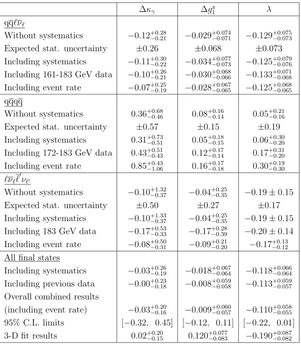
−1. After combining with our previous measurements at centre- of-mass energies of 161–183 GeV we obtain κ
γ=0.97
+0.20−0.16, g
1z=0.991
+0.060−0.057and λ= − 0.110
+0.058−0.055, where the errors include both statistical and systematic uncertainties and each coupling is determined by setting the other two couplings to their Standard Model values. These results are consistent with the Standard Model expectations.
(Submitted to the European Physical Journal C)
The OPAL Collaboration
G. Abbiendi
2, K. Ackerstaff
8, C. Ainsley
5, P.F. ˚ Akesson
3, G. Alexander
22, J. Allison
16, K.J. Anderson
9, S. Arcelli
17, S. Asai
23, S.F. Ashby
1, D. Axen
27, G. Azuelos
18,a, I. Bailey
26, A.H. Ball
8, E. Barberio
8, R.J. Barlow
16, S. Baumann
3, T. Behnke
25, K.W. Bell
20, G. Bella
22,
A. Bellerive
9, G. Benelli
2, S. Bentvelsen
8, S. Bethke
32, O. Biebel
32, I.J. Bloodworth
1, O. Boeriu
10, P. Bock
11, J. B¨ohme
14,h, D. Bonacorsi
2, M. Boutemeur
31, S. Braibant
8, P. Bright-Thomas
1, L. Brigliadori
2, R.M. Brown
20, H.J. Burckhart
8, J. Cammin
3, P. Capiluppi
2,
R.K. Carnegie
6, A.A. Carter
13, J.R. Carter
5, C.Y. Chang
17, D.G. Charlton
1,b, P.E.L. Clarke
15, E. Clay
15, I. Cohen
22, O.C. Cooke
8, J. Couchman
15, C. Couyoumtzelis
13, R.L. Coxe
9, A. Csilling
15,j, M. Cuffiani
2, S. Dado
21, G.M. Dallavalle
2, S. Dallison
16, A. de Roeck
8, E. de
Wolf
8, P. Dervan
15, K. Desch
25, B. Dienes
30,h, M.S. Dixit
7, M. Donkers
6, J. Dubbert
31, E. Duchovni
24, G. Duckeck
31, I.P. Duerdoth
16, P.G. Estabrooks
6, E. Etzion
22, F. Fabbri
2,
M. Fanti
2, L. Feld
10, P. Ferrari
12, F. Fiedler
8, I. Fleck
10, M. Ford
5, A. Frey
8, A. F¨ urtjes
8, D.I. Futyan
16, P. Gagnon
12, J.W. Gary
4, G. Gaycken
25, C. Geich-Gimbel
3, G. Giacomelli
2,
P. Giacomelli
8, D. Glenzinski
9, J. Goldberg
21, C. Grandi
2, K. Graham
26, E. Gross
24, J. Grunhaus
22, M. Gruw´e
25, P.O. G¨ unther
3, C. Hajdu
29, G.G. Hanson
12, M. Hansroul
8,
M. Hapke
13, K. Harder
25, A. Harel
21, M. Harin-Dirac
4, A. Hauke
3, M. Hauschild
8, C.M. Hawkes
1, R. Hawkings
8, R.J. Hemingway
6, C. Hensel
25, G. Herten
10, R.D. Heuer
25,
J.C. Hill
5, A. Hocker
9, K. Hoffman
8, R.J. Homer
1, A.K. Honma
8, D. Horv´ath
29,c, K.R. Hossain
28, R. Howard
27, P. H¨ untemeyer
25, P. Igo-Kemenes
11, K. Ishii
23, F.R. Jacob
20,
A. Jawahery
17, H. Jeremie
18, C.R. Jones
5, P. Jovanovic
1, T.R. Junk
6, N. Kanaya
23, J. Kanzaki
23, G. Karapetian
18, D. Karlen
6, V. Kartvelishvili
16, K. Kawagoe
23, T. Kawamoto
23, R.K. Keeler
26, R.G. Kellogg
17, B.W. Kennedy
20, D.H. Kim
19, K. Klein
11, A. Klier
24, S. Kluth
32,
T. Kobayashi
23, M. Kobel
3, T.P. Kokott
3, S. Komamiya
23, R.V. Kowalewski
26, T. Kress
4, P. Krieger
6, J. von Krogh
11, T. Kuhl
3, M. Kupper
24, P. Kyberd
13, G.D. Lafferty
16, H. Landsman
21, D. Lanske
14, I. Lawson
26, J.G. Layter
4, A. Leins
31, D. Lellouch
24, J. Letts
12, L. Levinson
24, R. Liebisch
11, J. Lillich
10, B. List
8, C. Littlewood
5, A.W. Lloyd
1, S.L. Lloyd
13,
F.K. Loebinger
16, G.D. Long
26, M.J. Losty
7, J. Lu
27, J. Ludwig
10, A. Macchiolo
18, A. Macpherson
28,m, W. Mader
3, S. Marcellini
2, T.E. Marchant
16, A.J. Martin
13, J.P. Martin
18,
G. Martinez
17, T. Mashimo
23, P. M¨attig
24, W.J. McDonald
28, J. McKenna
27, T.J. McMahon
1, R.A. McPherson
26, F. Meijers
8, P. Mendez-Lorenzo
31, W. Menges
25, F.S. Merritt
9, H. Mes
7, A. Michelini
2, S. Mihara
23, G. Mikenberg
24, D.J. Miller
15, W. Mohr
10, A. Montanari
2, T. Mori
23, K. Nagai
8, I. Nakamura
23, H.A. Neal
12,f, R. Nisius
8, S.W. O’Neale
1, F.G. Oakham
7, F. Odorici
2,
H.O. Ogren
12, A. Oh
8, A. Okpara
11, M.J. Oreglia
9, S. Orito
23, G. P´asztor
8,j, J.R. Pater
16, G.N. Patrick
20, J. Patt
10, P. Pfeifenschneider
14,i, J.E. Pilcher
9, J. Pinfold
28, D.E. Plane
8, B. Poli
2, J. Polok
8, O. Pooth
8, M. Przybycie´ n
8,d, A. Quadt
8, C. Rembser
8, P. Renkel
24, H. Rick
4,
N. Rodning
28, J.M. Roney
26, S. Rosati
3, K. Roscoe
16, A.M. Rossi
2, Y. Rozen
21, K. Runge
10, O. Runolfsson
8, D.R. Rust
12, K. Sachs
6, T. Saeki
23, O. Sahr
31, E.K.G. Sarkisyan
22, C. Sbarra
26,
A.D. Schaile
31, O. Schaile
31, P. Scharff-Hansen
8, M. Schr¨oder
8, M. Schumacher
25, C. Schwick
8, W.G. Scott
20, R. Seuster
14,h, T.G. Shears
8,k, B.C. Shen
4, C.H. Shepherd-Themistocleous
5,
P. Sherwood
15, G.P. Siroli
2, A. Skuja
17, A.M. Smith
8, G.A. Snow
17, R. Sobie
26, S. S¨oldner-Rembold
10,e, S. Spagnolo
20, M. Sproston
20, A. Stahl
3, K. Stephens
16, K. Stoll
10, D. Strom
19, R. Str¨ohmer
31, L. Stumpf
26, B. Surrow
8, S.D. Talbot
1, S. Tarem
21, R.J. Taylor
15,
R. Teuscher
9, M. Thiergen
10, J. Thomas
15, M.A. Thomson
8, E. Torrence
9, S. Towers
6,
D. Toya
23, T. Trefzger
31, I. Trigger
8, Z. Tr´ocs´anyi
30,g, E. Tsur
22, M.F. Turner-Watson
1,
I. Ueda
23, B. Vachon26, P. Vannerem
10, M. Verzocchi
8, H. Voss
8, J. Vossebeld
8, D. Waller
6,
C.P. Ward
5, D.R. Ward
5, P.M. Watkins
1, A.T. Watson
1, N.K. Watson
1, P.S. Wells
8, T. Wengler
8, N. Wermes
3, D. Wetterling
11J.S. White
6, G.W. Wilson
16, J.A. Wilson
1,
T.R. Wyatt
16, S. Yamashita
23, V. Zacek
18, D. Zer-Zion
8,l1
School of Physics and Astronomy, University of Birmingham, Birmingham B15 2TT, UK
2
Dipartimento di Fisica dell’ Universit`a di Bologna and INFN, I-40126 Bologna, Italy
3
Physikalisches Institut, Universit¨at Bonn, D-53115 Bonn, Germany
4
Department of Physics, University of California, Riverside CA 92521, USA
5
Cavendish Laboratory, Cambridge CB3 0HE, UK
6
Ottawa-Carleton Institute for Physics, Department of Physics, Carleton University, Ottawa, Ontario K1S 5B6, Canada
7
Centre for Research in Particle Physics, Carleton University, Ottawa, Ontario K1S 5B6, Canada
8
CERN, European Organisation for Nuclear Research, CH-1211 Geneva 23, Switzerland
9
Enrico Fermi Institute and Department of Physics, University of Chicago, Chicago IL 60637, USA
10
Fakult¨at f¨ ur Physik, Albert Ludwigs Universit¨at, D-79104 Freiburg, Germany
11
Physikalisches Institut, Universit¨at Heidelberg, D-69120 Heidelberg, Germany
12
Indiana University, Department of Physics, Swain Hall West 117, Bloomington IN 47405, USA
13
Queen Mary and Westfield College, University of London, London E1 4NS, UK
14
Technische Hochschule Aachen, III Physikalisches Institut, Sommerfeldstrasse 26-28, D-52056 Aachen, Germany
15
University College London, London WC1E 6BT, UK
16
Department of Physics, Schuster Laboratory, The University, Manchester M13 9PL, UK
17
Department of Physics, University of Maryland, College Park, MD 20742, USA
18
Laboratoire de Physique Nucl´eaire, Universit´e de Montr´eal, Montr´eal, Quebec H3C 3J7, Canada
19
University of Oregon, Department of Physics, Eugene OR 97403, USA
20
CLRC Rutherford Appleton Laboratory, Chilton, Didcot, Oxfordshire OX11 0QX, UK
21
Department of Physics, Technion-Israel Institute of Technology, Haifa 32000, Israel
22
Department of Physics and Astronomy, Tel Aviv University, Tel Aviv 69978, Israel
23
International Centre for Elementary Particle Physics and Department of Physics, University of Tokyo, Tokyo 113-0033, and Kobe University, Kobe 657-8501, Japan
24
Particle Physics Department, Weizmann Institute of Science, Rehovot 76100, Israel
25
Universit¨at Hamburg/DESY, II Institut f¨ ur Experimental Physik, Notkestrasse 85, D-22607 Hamburg, Germany
26
University of Victoria, Department of Physics, P O Box 3055, Victoria BC V8W 3P6, Canada
27
University of British Columbia, Department of Physics, Vancouver BC V6T 1Z1, Canada
28
University of Alberta, Department of Physics, Edmonton AB T6G 2J1, Canada
29
Research Institute for Particle and Nuclear Physics, H-1525 Budapest, P O Box 49, Hungary
30
Institute of Nuclear Research, H-4001 Debrecen, P O Box 51, Hungary
31
Ludwigs-Maximilians-Universit¨at M¨ unchen, Sektion Physik, Am Coulombwall 1, D-85748 Garching, Germany
32
Max-Planck-Institute f¨ ur Physik, F¨ohring Ring 6, 80805 M¨ unchen, Germany
a
and at TRIUMF, Vancouver, Canada V6T 2A3
b
and Royal Society University Research Fellow
c
and Institute of Nuclear Research, Debrecen, Hungary
d
and University of Mining and Metallurgy, Cracow
e
and Heisenberg Fellow
f
now at Yale University, Dept of Physics, New Haven, USA
g
and Department of Experimental Physics, Lajos Kossuth University, Debrecen, Hungary
h
and MPI M¨ unchen
i
now at MPI f¨ ur Physik, 80805 M¨ unchen
j
and Research Institute for Particle and Nuclear Physics, Budapest, Hungary
k
now at University of Liverpool, Dept of Physics, Liverpool L69 3BX, UK
l
and University of California, Riverside, High Energy Physics Group, CA 92521, USA
m
and CERN, EP Div, 1211 Geneva 23.
1 Introduction
W-pair production in e
+e
−annihilation involves, in addition to the t-channel ν-exchange, the triple gauge boson vertices WWγ and WWZ which are present in the Standard Model due to its non-Abelian nature. Since the start of LEP operation at and above the W-pair threshold several measurements have been made of the triple gauge boson couplings ( TGC s) involved with these vertices in W-pair production [1–4], single W and single photon production [5].
Limits on TGC s also exist from studies of di-boson production at the Tevatron [6]. In this paper we update our previous measurements [1–3] to include the data collected during 1998 at a centre-of-mass energy of 189 GeV with an integrated luminosity of 183 pb
−1.
According to the most general Lorentz invariant Lagrangian [7–10] there can be seven in- dependent couplings describing each of the WWγ and WWZ vertices. This large parameter space can be reduced by requiring the Lagrangian to satisfy electromagnetic gauge invariance and charge conjugation as well as parity invariance. The number of parameters reduces to five, which can be taken as g
1z, κ
z, κ
γ, λ
zand λ
γ[7, 8]. These parameters are directly related to the W electromagnetic and weak properties [8, 9]. In the Standard Model g
1z=κ
z=κ
γ=1 and λ
z=λ
γ=0. Precision measurements on the Z
0resonance and lower energy data, are consistent with the following SU(2) × U(1) relations between the five couplings [7, 9],
∆κ
z= − ∆κ
γtan
2θ
w+ ∆g
1z, λ
z= λ
γ.
Here ∆ indicates a deviation of the respective quantity from its Standard Model value and θ
wis the weak mixing angle. These two relations leave only three independent couplings, ∆κ
γ,
∆g
1zand λ(=λ
γ=λ
z) which are not significantly restricted [11, 12] by existing LEP and SLC Z
0data.
Anomalous TGC s give different contributions to different helicity states of the outgoing W- bosons. Consequently they affect the angular distributions of the produced W bosons and their decay products, as well as the total W-pair cross-section. Ignoring the effects of the finite W width and the initial state radiation (ISR), the production and decay of W bosons is completely described by five angles. Conventionally these are taken to be [7, 9, 13]: the W
−production polar angle
1θ
W; the polar and azimuthal angles, θ
1∗and φ
∗1, of the decay fermion from the W
−in the W
−rest frame
2; and the analogous angles for the anti-fermion from the W
+decay, θ
2∗and φ
∗2. However for W-pairs observed in the detector, the experimental accessibility of these angles and therefore the sensitivity to the TGC s, is limited and depends strongly on the final state produced when the W bosons decay.
In this study all final states are used, namely the fully leptonic, ℓν
ℓℓ
′ν
ℓ′, the semileptonic, qqℓν
ℓ, and the fully hadronic, qqqq final states, with branching fractions of 10.6%, 43.9% and 45.6% respectively. This study is divided into two parts. In the first part the W-pair event rate
1The OPAL right-handed coordinate system is defined such that the origin is at the geometric centre of the detector, thez-axis is parallel to, and has positive sense, along the e−beam direction,θis the polar angle with respect toz andφis the azimuthal angle aroundz.
2 The axes of the right-handed coordinate system in the W rest-frame are defined such thatz is along the parent W flight direction and y is in the direction−→
e−×−W→where −→
e− is the electron beam direction and −W→ is the parent W flight direction.
for each of the three final states is analysed in terms of the TGC s. The second part is a study of the W-pair event shape for each final state using optimal observables.
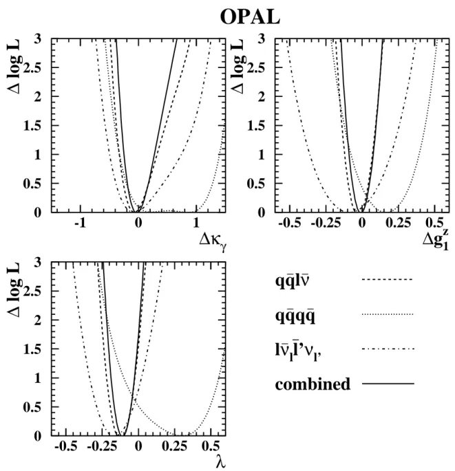
Most of the TGC results of this analysis are obtained for each of the three couplings sep- arately, setting the other two couplings to their Standard Model values. These results will be presented in tables and log L curves
3. We also perform two-dimensional and three-dimensional fits, where two or all three TGC parameters are allowed to vary in the fits. The results of these fits will be presented by contour plots.
The following section includes a short presentation of the OPAL data and Monte Carlo samples and in section 3 the analysis of the W-pair event rate is described. Moving on to the event shape analysis, the first step, namely the event reconstruction, is presented in section 4. The TGC extraction using the technique of optimal observables is explained in section 5.
Systematic errors are described in section 6 and the combined TGC results are presented in section 7. Section 8 summarises the results of this study.
2 Data and Monte Carlo models
The data were acquired during 1998 with the OPAL detector which is described in detail elsewhere [14]. The integrated luminosity, evaluated using small angle Bhabha scattering events observed in the silicon tungsten forward calorimeter, is 183.05 ± 0.40 pb
−1. The luminosity- weighted mean centre-of-mass energy for the data sample is √
s=188.64 ± 0.04 GeV.
In the analyses described below, a number of Monte Carlo models are used to provide estimates of efficiencies and backgrounds as well as the expected W-pair production and decay angular distributions for different TGC values. The majority of the Monte Carlo samples were generated at √
s = 189 GeV with M
W= 80.33 GeV / c
2. All Monte Carlo samples mentioned below were processed by the full OPAL simulation program [15] and then subjected to the same reconstruction procedure as the data.
The main Monte Carlo program used in this analysis is the E xcalibur [16] generator. This program generates all four-fermion final states using the full set of electroweak diagrams in- cluding the W
+W
−production diagrams (class
4CC03) and other four-fermion graphs, such as e
+e
−→ Weν
e, e
+e
−→ Z
0e
+e
−and e
+e
−→ Z
0Z
0. Using this program, samples were generated with and without anomalous TGC s. Each sample was generated with a different set of TGC values. These samples are used to calculate the TGC dependence of the expected event rate and angular distributions. We also apply a reweighting technique based on the matrix element corresponding to all the contributing four-fermion diagrams. In this way, the angular distri- butions for any particular set of anomalous couplings are obtained from Monte Carlo samples generated at a limited number of different TGC values.
For systematic studies we use Standard Model four-fermion samples generated by the grc4f [17] and K oralw [18] programs. K oralw uses the same matrix element as grc4f
3 Throughout this paper, logLdenotes negative log-likelihood.
4 In this paper, the W pair production diagrams,i.e. t-channelνe exchange and s-channel Z0/γ exchange, are referred to as “CC03”, following the notation of [7].
but has the most complete simulation of ISR out of all the four-fermion Monte Carlo programs used in this analysis. The efficiency obtained from the K oralw sample is used to correct the expected event rate. To estimate the hadronisation systematics, Monte Carlo samples were produced by grc4f including the CC03 diagrams only, and the fragmentation stage was gener- ated separately with either J etset [19] or H erwig [20]. To study final state interaction effects in qqqq events we used Monte Carlo samples with different implementations of Bose-Einstein correlations and colour reconnection effects, as detailed in section 6.
There are other background sources not associated with four-fermion processes. The main one, Z
0/γ → qq, including higher order QCD diagrams, is simulated using P ythia , with H erwig used as an alternative to study possible systematic effects. Other background pro- cesses involving two fermions in the final state are studied using K oralz [21] for e
+e
−→ µ
+µ
−, e
+e
−→ τ
+τ
−and e
+e
−→ νν , and B hwide [22] for e
+e
−→ e
+e
−. Backgrounds from two-photon processes are evaluated using P ythia , H erwig , P hojet [23] and the Vermaseren genera- tor [24]. It is assumed that the centre-of-mass energy of 189 GeV is below the threshold for Higgs boson production.
3 Event rate TGC analysis
The event rate analysis is based on the total W
+W
−production cross-section measurement [25].
We use here the same selection with the same efficiency and background estimates. The dif- ference is only in the physics interpretation. To analyse the W
+W
−event rate, all three final states are used. Each final state corresponds to a different selection algorithm. These algo- rithms are similar to those used at lower centre-of-mass energies (see [3] and references therein) and the differences are described in [25].
The results are summarised in Table 1. The efficiencies refer to CC03 W
+W
−events and include cross contamination between the three final states. To calculate the expected num- bers of events we use our total integrated luminosity of 183.05 ± 0.40 pb
−1and the total W
+W
−production cross-section value of 16.26 pb corresponding to our centre-of-mass energy of 188.64 ± 0.04 GeV and a W mass of M
W=80.42 ± 0.07 GeV / c
2measured at the Tevatron
5[26].
The cross-section calculation is done using the R acoon WW [27] and Y fs WW3 [28] Monte Carlo programs which include the most complete O (α) radiative corrections using the double pole approximation method. The results obtained by these two independent programs agree within 0.1% [29]. Furthermore the theoretical uncertainty of 0.42% is improved compared with the 2% uncertainty of the G entle [30] semi-analytic program which has been used in our previous publications. However, since we have not yet been able to study the full effect of our selection cuts with these recent Monte Carlo generators, we prefer not to reduce our assumed theoretical uncertainty of 2% which has only a negligible effect on our final results.
The four-fermion background is split between final states with and without contributions from diagrams containing a triple gauge boson vertex. For each of the three final states in our signal the TGC -dependent background is calculated from the difference between the accepted
5 The LEP results for the W mass are not used for the
TGC
measurement, since they have been obtained under the assumption that W pairs are produced according to the Standard Model, whereas W production at the Tevatron does not involve the triple gauge vertex.Selected as W
+W
−→ ℓν
ℓℓ
′ν
ℓ′W
+W
−→ qqℓν
ℓW
+W
−→ qqqq Combined Efficiency [%] 82.3 ± 1.2 87.7 ± 0.9 86.5 ± 0.8 86.6 ± 0.6
Signal events 258 ± 6 1145 ± 26 1175 ± 26 2578 ± 55
Background events:
4-fermion, TGC -dep. 17 ± 2 27 ± 4 10 ± 6 54 ± 7
4-fermion, TGC -indep. 7.0 ± 0.3 34 ± 3 71 ± 10 111 ± 9
Z
0/γ → ff 4.1 ± 0.3 48 ± 6 245 ± 17 297 ± 17
Two-photon 0.9 ± 0.9 3 ± 3 0 4 ± 4
Total background 29 ± 3 112 ± 9 325 ± 21 466 ± 24
Total expected 287 ± 7 1257 ± 27 1500 ± 33 3044 ± 60
Observed 276 1246 1546 3068
Table 1: Expected and observed numbers of events in each W
+W
−final state for an integrated luminosity of 183.05 ± 0.40 pb
−1at 188.64 ± 0.04 GeV, assuming M
W= 80.42 ± 0.07 GeV / c
2and Standard Model branching fractions. The efficiency values and the numbers of signal events include cross contamination between the three final states. The errors on the combined numbers account for correlations between the systematic errors for different final states.
four-fermion cross-section (including all diagrams) and the accepted CC03 cross-section. The background from other final states
6does not depend on the TGC s.
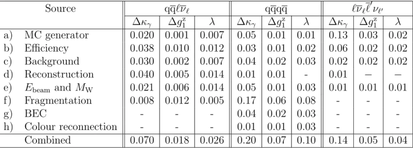
The errors listed in Table 1 are due to Monte Carlo statistics, luminosity uncertainty of 0.2%, theoretical uncertainty in the total cross-section (2%), centre-of-mass energy and W mass uncertainties (0.04% of the total cross-section each), data/MC differences, tracking losses, detector occupancy and fragmentation uncertainties. A detailed description of all these sources can be found in [25].
The total number of expected events in each final state is consistent with the corresponding number of observed events. Therefore, there is no evidence for any significant contribution from anomalous couplings. A quantitative study of TGC s from the W-pair event yield is performed by comparing the numbers of observed events in each of the three event selection channels with the expected numbers which are parametrised as second-order polynomials in the TGC s. This parametrisation is based on the linear dependence of the triple gauge vertex Lagrangian on the TGC s, corresponding to a second-order polynomial dependence of the cross-section. Conse- quently, the expected number of events for each final state also has a second-order polynomial dependence on the TGC s. The polynomial coefficients are calculated from the expected number of events at different TGC values, as obtained from the corresponding E xcalibur Monte Carlo samples. For each final state, the corresponding expected cross section is normalised to the Standard Model expectation (sum of signal and TGC -dependent background) listed in Table 1.
The primary reason for this normalisation is the fact that when calculating the numbers in Table 1, R acoon WW and Y fs WW3 are used for the cross-section and K oralw for the ef- ficiency. This is considered to be more complete than E xcalibur . The normalisation factor varies between 0.970 (ℓν
ℓℓ
′ν
ℓ′selection) and 0.987 (qqqq selection).
The probability to observe the measured number of candidates, given the expected value,
6 A small contribution from the νeνeff final states which are partly produced by the W fusion diagram is included in the
TGC
-dependent background.is calculated using a Poisson distribution. The product of the three probability distributions corresponding to the three final states is taken as the event rate likelihood function. The systematic uncertainties are incorporated into the TGC fit by allowing the expected numbers of signal and background events to vary in the fit and constraining them to have a Gaussian distribution around their expected values with their systematic errors taken as the width of the distributions. The systematic uncertainties, excluding those on efficiency and background, are assumed to be correlated between the three different event selections.
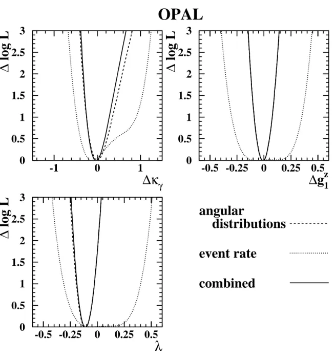
Data from lower centre-of-mass energies are included, assuming all systematic errors to be fully correlated between energies. The corresponding log L curves are used in combination with the results of the event shape analysis, which is described in the following sections. The full set of results is then presented in Figure 7, where the event rate contributions are shown as dotted lines
7.
4 Event reconstruction
Starting from the event sample used for the event-rate analysis, a reconstruction is performed to extract the maximum possible information on the W production and decay angles, which are then used to extract the couplings. Events which cannot be well reconstructed are rejected from the sample.
Three kinematic fits with different sets of requirements are used in the event reconstruction:
A. requiring conservation of energy and momentum, neglecting ISR;
B. additionally constraining the reconstructed masses of the two W-bosons to be equal;
C. additionally constraining each reconstructed W mass to the average value measured at the Tevatron, M
W=80.42 GeV / c
2[26].
For qqqq events, where all four final state fermions are measurable, fits A, B and C have 4, 5 and 6 constraints respectively. For qqeν
eand qqµν
µevents the number of constraints is reduced by 3 due to the invisible neutrino. For qqτ ν
τevents there is at least one additional unobserved neutrino from the τ decay, but the momentum sum of the track(s) assigned to the τ can still be used as an approximation to the τ flight direction, relying on its high boost. The τ energy is left unknown, resulting in a further loss of one constraint. Finally for ℓν
ℓℓ
′ν
ℓ′events, where none of the leptons is a τ, there are two invisible neutrinos. Hence, six constraints are lost and requirement C is needed.
In the following we discuss the reconstruction of each final state separately.
7 The logL curves are expected to be symmetric around the event rate minimum position which, in most cases, is very close to the Standard Model
TGC
value. However, for the ∆κγ parameter, the event rate acquires its minimum at positive ∆κγvalue. The exact location of this minimum differs betweenℓνℓℓ′νℓ′ qqℓνℓand qqqq events due to contributions from non-CC03 diagrams. Therefore, the overall logL(∆κγ) function summed over the three final states is no longer symmetric, unlike the corresponding functions for the otherTGC
parameters.4.1 Reconstruction of qqℓν
ℓfinal states
Candidate qqeν
eand qqµν
µevents without a well reconstructed lepton track, which were included in the sample used for the event rate analysis, are removed from the present sample.
In this way, each of the events left in the sample has one track that is identified as the most likely lepton candidate. For the case of qqτ ν
τevents, either one track or a narrow jet consisting of three tracks is assigned as the τ decay product.
The electron direction is reconstructed by the tracking detectors and the energy is measured in the electromagnetic calorimeters. For muons the momentum is measured using the tracking detectors. As explained above, the direction of τ candidates can be directly reconstructed whilst the energy can only be derived from a kinematic fit.
The remaining tracks and calorimeter clusters in the event are grouped into two jets using the Durham k
⊥algorithm [31]. The total energy and momentum of each of the jets are calculated with the method described in [32]. Kinematic fit A, requiring energy-momentum conservation, is then performed on the events. The qqeν
eand qqµν
µevents are accepted if this one-constraint fit converges with a probability larger than 0.001. This cut rejects about 2% of the signal events and 4% of the background.
To improve the resolution in the angular observables used for the TGC analysis, kinematic fit C is performed on qqeν
eand qqµν
µevents. The W-mass constraint in this fit allows for the finite W-width
8. We demand that the kinematic fit converges with a probability larger than 0.001. For the 4% of events which fail at this point we revert to using the results of fit A.
For qqτ ν
τevents the kinematic fit B is performed and required to converge with a probability larger than 0.025. This cut rejects 14% of the signal and 41% of the background. Furthermore, this cut suppresses those qqτ ν
τevents which are correctly identified as belonging to this decay channel but where the τ decay products are not identified correctly, leading to an incorrect estimate of the τ flight direction or its charge. The fraction of such events in the qqτ ν
τsample is reduced from 18% to 12%.
Out of the original number of 1246 qqℓν
ℓcandidates used for the event rate analysis there are 1075 events left (368 qqeν
e, 387 qqµν
µand 320 qqτ ν
τ) after all these cuts. Assuming Standard Model cross-sections for signal and background processes, the remaining background fraction is 4.6%. This does not include cross-migration between the three lepton channels. The background sources are: four-fermion processes after subtracting the contribution from the CC03 diagrams (2.4%), Z
0/γ → qq (2.4%), W
+W
−→ qqqq and ℓν
ℓℓ
′ν
ℓ′(0.2%) and two-photon reactions (0.1%).
In the reconstruction of the qqℓν
ℓevents we obtain cos θ
Wby summing the kinematically fitted four-momenta of the two jets. The decay angles of the leptonically decaying W are obtained from the charged lepton four-momentum, after boosting back to the parent W rest frame. For the hadronically decaying W we are left with a two-fold ambiguity in assigning the
8 The W mass distribution is treated as a Gaussian in the kinematic fit. However, in order to simulate the expected Breit-Wigner form of the W mass spectrum, the variance of the Gaussian is updated at each iteration of the kinematic fit in such a way that the probabilities of observing the current fitted W mass are equal whether calculated using the Gaussian distribution or using a Breit-Wigner.
jets to the quark and antiquark. This ambiguity is taken into account in the analyses described below.
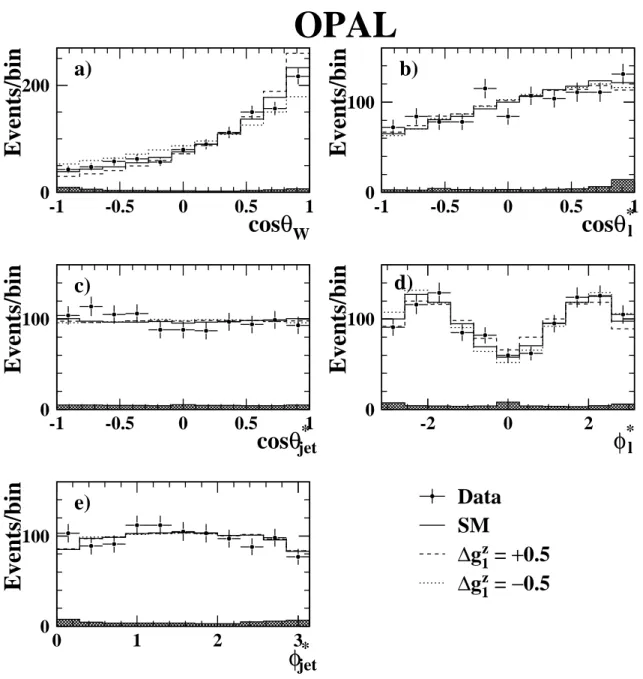
In Figure 1 we show the distributions of all the five angles obtained from the combined qqℓν
ℓevent sample, and the expected distributions for ∆g
1z= ± 0.5 and 0. These expected distributions are obtained from fully simulated Monte Carlo event samples generated with E xcalibur , normalised to the number of events observed in the data. Sensitivity to TGC s is observed mainly for cos θ
W. The contribution of cos θ
∗ℓ, φ
∗ℓ, cos θ
jet∗and φ
∗jetto the overall sensitivity enters mainly through their correlations with cos θ
W.
4.2 Reconstruction of qqqq final states
Using the Durham k
⊥algorithm [31], each selected qqqq candidate is reconstructed as four jets, whose energies are corrected for the double counting of charged track momenta and calorimeter energies [33]. These four jets can be paired into W-bosons in three possible ways. To improve the resolution on the jet four-momentum we perform for each possible jet pairing the five- constraint kinematic fit B. We require at least one jet pairing with a successful fit yielding a W-mass between 70 and 90 GeV. The W charge is assigned by comparing the sum of the charges of the two jets coming from the same W candidate. More details are described in [3].
The correct di-jet pairing is identified by a likelihood algorithm [34] which takes into account correlations between the input variables. We use as input to our likelihood the W candidate mass as obtained from the kinematic fit B, the angles between the two jets coming from each W candidate, the difference between the W candidate masses as obtained from the kinematic fit A and the charge difference between the two W candidates. According to the W
+W
−E xcalibur Monte Carlo, the probability of selecting the correct di-jet combination is about 79%, and the probability of correct assignment of the W charge, once the correct pairing has been chosen, is about 77%.
The fraction of events correctly reconstructed can be increased by cutting on the value L of the jet pairing likelihood. Its distribution is shown in Figure 2(a). We cut at L > 0.5, which minimises the expected total errors on the measured TGC s.
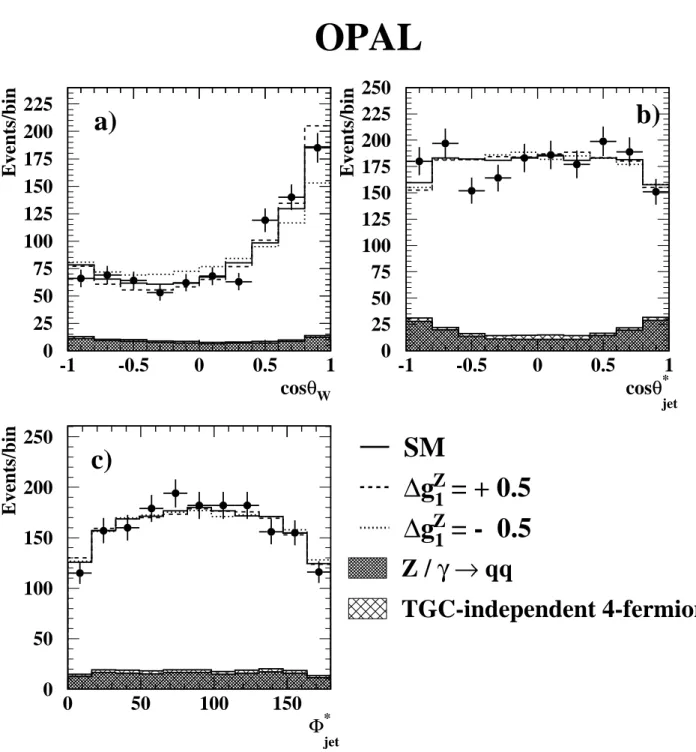
After all cuts the probability of correct pairing increases to 87% and the probability of correct determination of the W charge is about 82%. The selection efficiency is reduced by these cuts from 86% to 54%, whereas the background drops from 23% to 12%. In the data, 889 events survive all cuts out of the 1546 initially selected. The distribution of the W charge separation is shown in Figure 2(b). The distributions of the variables cos θ
W, cos θ
jet∗and φ
∗jetare shown in Figure 3.
4.3 Reconstruction of ℓν
ℓℓ
′ν
ℓ′final states
As explained above, the reconstruction of ℓν
ℓℓ
′ν
ℓ′final states is possible only by using kinematic
fit C for the case of no τ-lepton in the final state. To reject events with τ -leptons we use
the lepton identification algorithm designed for the W branching ratio measurement [25]. In
addition, events with only one reconstructed cone which were accepted for the event rate analysis are removed from the sample. As a result of these two cuts, the number of data events drops from 276 to 133. The efficiency for ℓν
ℓℓ
′ν
ℓ′events with ℓ =e,µ drops from 89% to 74%. The contamination left in the sample from ℓν
ℓℓ
′ν
ℓ′final states with a τ -lepton is 14% and the background from other final states is only 0.5%.
Kinematic fit C has no constraints and turns into solving a quadratic equation. In the ideal case of no measurement errors and satisfying the conditions where fit C is valid, namely no ISR and narrow W width, one expects to obtain two real solutions corresponding to a two-fold ambiguity in the angle set cos θ
W, φ
∗1and φ
∗2. There is no ambiguity in the angles θ
∗1and θ
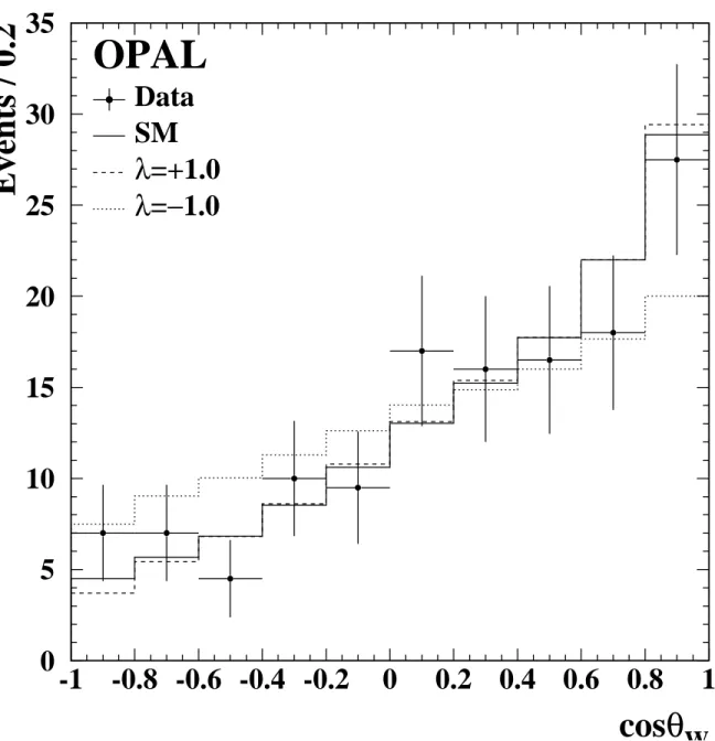
2∗which have a one-to-one correspondence with the lepton momenta. In realistic conditions, however, including ISR, finite W width and measurement errors, one might obtain no real solution, but a pair of complex conjugate solutions. In fact, only 92 out of 133 events in the data have two real solutions, in agreement with the Monte Carlo expectation of 97.8 events. In the complex solution case, the nearest real solution is taken by setting the imaginary parts of the complex solutions to zero.
Figure 4 shows the reconstructed cos θ
Wdistribution. The data distribution agrees with the Standard Model expectation.
5 Event shape TGC analysis
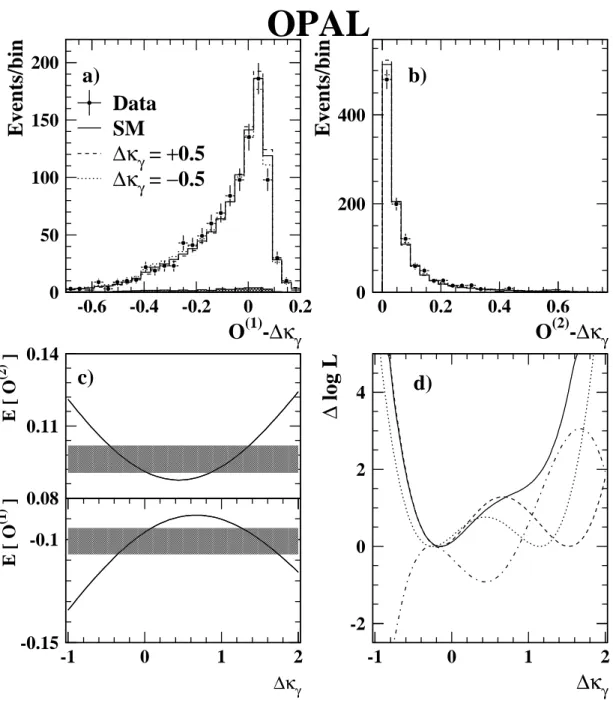
The angular distributions from all final states are consistent with the Standard Model expecta- tion and no evidence is seen for any significant contributions from anomalous couplings. For a quantitative study we use the method of optimal observables based on the following dependence of the W-pair differential cross-section on the TGC s,
dσ(Ω, α) = S
(0)(Ω) +
Xi
α
i· S
i(1)(Ω) +
Xi,j