Measurement of W boson polarisations and CP-violating triple gauge couplings from W

arXiv:hep-ex/0009021v1 7 Sep 2000

EUROPEAN ORGANIZATION FOR NUCLEAR RESEARCH

CERN-EP-2000-113 18 August, 2000

Measurement of W boson polarisations and CP-violating triple gauge

couplings from W

W

production at LEP

The OPAL Collaboration

Abstract

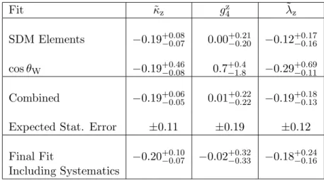
Measurements are presented of the polarisation of W⁺W⁻ boson pairs produced in e⁺e⁻ collisions, and of CP-violating WWZ and WWγ trilinear gauge couplings. The data were recorded by the OPAL experiment at LEP during 1998, where a total integrated luminosity of 183 pb⁻¹ was obtained at a centre-of-mass energy of 189 GeV. The measurements are performed through a spin density matrix analysis of the W boson decay products. The fraction of W bosons produced with longitudinal polarisation was found to be σ_L/σ_total = (21.0±3.3±1.6)% where the first error is statistical and the second systematic. The joint W boson pair production fractions were found to be σ_TT/σ_total = (78.1 ±9.0 ±3.2)%, σ_LL/σ_total = (20.1 ±7.2±1.8)% and σ_TL/σ_total = (1.8±14.7 ±3.8)%. In the CP-violating trilinear gauge coupling sector we find ˜κ_z =−0.20^+0.10−0.07, g₄^z = −0.02^+0.32−0.33 and ˜λ_z =

−0.18^+0.24−0.16, where errors include both statistical and systematic uncertainties. In each case the coupling is determined with all other couplings set to their Standard Model values except those related to the measured coupling via SU(2)_L×U(1)_Y symmetry. These results are consistent with Standard Model expectations.

(To be submitted to Eur. Phys. J. C )

The OPAL Collaboration

G. Abbiendi², K. Ackerstaff⁸, C. Ainsley⁵, P.F. ˚Akesson³, G. Alexander²², J. Allison¹⁶,

K.J. Anderson⁹, S. Arcelli¹⁷, S. Asai²³, S.F. Ashby¹, D. Axen²⁷, G. Azuelos^18,a, I. Bailey²⁶, A.H. Ball⁸, E. Barberio⁸, R.J. Barlow¹⁶, S. Baumann³, T. Behnke²⁵, K.W. Bell²⁰, G. Bella²², A. Bellerive⁹,

G. Benelli², S. Bentvelsen⁸, S. Bethke³², O. Biebel³², I.J. Bloodworth¹, O. Boeriu¹⁰, P. Bock¹¹, J. B¨ohme^14,h, D. Bonacorsi², M. Boutemeur³¹, S. Braibant⁸, P. Bright-Thomas¹, L. Brigliadori²,

R.M. Brown²⁰, H.J. Burckhart⁸, J. Cammin³, P. Capiluppi², R.K. Carnegie⁶, A.A. Carter¹³, J.R. Carter⁵, C.Y. Chang¹⁷, D.G. Charlton^1,b, P.E.L. Clarke¹⁵, E. Clay¹⁵, I. Cohen²², O.C. Cooke⁸,

J. Couchman¹⁵, C. Couyoumtzelis¹³, R.L. Coxe⁹, A. Csilling^15,j, M. Cuffiani², S. Dado²¹, G.M. Dallavalle², S. Dallison¹⁶, A. de Roeck⁸, E. de Wolf⁸, P. Dervan¹⁵, K. Desch²⁵, B. Dienes^30,h,

M.S. Dixit⁷, M. Donkers⁶, J. Dubbert³¹, E. Duchovni²⁴, G. Duckeck³¹, I.P. Duerdoth¹⁶, P.G. Estabrooks⁶, E. Etzion²², F. Fabbri², M. Fanti², L. Feld¹⁰, P. Ferrari¹², F. Fiedler⁸, I. Fleck¹⁰,

M. Ford⁵, A. Frey⁸, A. F¨urtjes⁸, D.I. Futyan¹⁶, P. Gagnon¹², J.W. Gary⁴, G. Gaycken²⁵, C. Geich-Gimbel³, G. Giacomelli², P. Giacomelli⁸, D. Glenzinski⁹, J. Goldberg²¹, C. Grandi², K. Graham²⁶, E. Gross²⁴, J. Grunhaus²², M. Gruw´e²⁵, P.O. G¨unther³, C. Hajdu²⁹, G.G. Hanson¹²,

M. Hansroul⁸, M. Hapke¹³, K. Harder²⁵, A. Harel²¹, M. Harin-Dirac⁴, A. Hauke³, M. Hauschild⁸, C.M. Hawkes¹, R. Hawkings⁸, R.J. Hemingway⁶, C. Hensel²⁵, G. Herten¹⁰, R.D. Heuer²⁵, J.C. Hill⁵, A. Hocker⁹, K. Hoffman⁸, R.J. Homer¹, A.K. Honma⁸, D. Horv´ath^29,c, K.R. Hossain²⁸, R. Howard²⁷,

P. H¨untemeyer²⁵, P. Igo-Kemenes¹¹, K. Ishii²³, F.R. Jacob²⁰, A. Jawahery¹⁷, H. Jeremie¹⁸, C.R. Jones⁵, P. Jovanovic¹, T.R. Junk⁶, N. Kanaya²³, J. Kanzaki²³, G. Karapetian¹⁸, D. Karlen⁶, V. Kartvelishvili¹⁶, K. Kawagoe²³, T. Kawamoto²³, R.K. Keeler²⁶, R.G. Kellogg¹⁷, B.W. Kennedy²⁰,

D.H. Kim¹⁹, K. Klein¹¹, A. Klier²⁴, S. Kluth³², T. Kobayashi²³, M. Kobel³, T.P. Kokott³, S. Komamiya²³, R.V. Kowalewski²⁶, T. Kress⁴, P. Krieger⁶, J. von Krogh¹¹, T. Kuhl³, M. Kupper²⁴,

P. Kyberd¹³, G.D. Lafferty¹⁶, H. Landsman²¹, D. Lanske¹⁴, I. Lawson²⁶, J.G. Layter⁴, A. Leins³¹, D. Lellouch²⁴, J. Letts¹², L. Levinson²⁴, R. Liebisch¹¹, J. Lillich¹⁰, B. List⁸, C. Littlewood⁵, A.W. Lloyd¹, S.L. Lloyd¹³, F.K. Loebinger¹⁶, G.D. Long²⁶, M.J. Losty⁷, J. Lu²⁷, J. Ludwig¹⁰, A. Macchiolo¹⁸, A. Macpherson^28,m, W. Mader³, S. Marcellini², T.E. Marchant¹⁶, A.J. Martin¹³,

J.P. Martin¹⁸, G. Martinez¹⁷, T. Mashimo²³, P. M¨attig²⁴, W.J. McDonald²⁸, J. McKenna²⁷, T.J. McMahon¹, R.A. McPherson²⁶, F. Meijers⁸, P. Mendez-Lorenzo³¹, W. Menges²⁵, F.S. Merritt⁹,

H. Mes⁷, A. Michelini², S. Mihara²³, G. Mikenberg²⁴, D.J. Miller¹⁵, W. Mohr¹⁰, A. Montanari², T. Mori²³, K. Nagai⁸, I. Nakamura²³, H.A. Neal^12,f, R. Nisius⁸, S.W. O’Neale¹, F.G. Oakham⁷, F. Odorici², H.O. Ogren¹², A. Oh⁸, A. Okpara¹¹, M.J. Oreglia⁹, S. Orito²³, G. P´asztor^8,j, J.R. Pater¹⁶,

G.N. Patrick²⁰, J. Patt¹⁰, P. Pfeifenschneider^14,i, J.E. Pilcher⁹, J. Pinfold²⁸, D.E. Plane⁸, B. Poli², J. Polok⁸, O. Pooth⁸, M. Przybycie´n^8,d, A. Quadt⁸, C. Rembser⁸, P. Renkel²⁴, H. Rick⁴, N. Rodning²⁸,

J.M. Roney²⁶, S. Rosati³, K. Roscoe¹⁶, A.M. Rossi², Y. Rozen²¹, K. Runge¹⁰, O. Runolfsson⁸, D.R. Rust¹², K. Sachs⁶, T. Saeki²³, O. Sahr³¹, E.K.G. Sarkisyan²², C. Sbarra²⁶, A.D. Schaile³¹,

O. Schaile³¹, P. Scharff-Hansen⁸, M. Schr¨oder⁸, M. Schumacher²⁵, C. Schwick⁸, W.G. Scott²⁰, R. Seuster^14,h, T.G. Shears^8,k, B.C. Shen⁴, C.H. Shepherd-Themistocleous⁵, P. Sherwood¹⁵, G.P. Siroli², A. Skuja¹⁷, A.M. Smith⁸, G.A. Snow¹⁷, R. Sobie²⁶, S. S¨oldner-Rembold^10,e, S. Spagnolo²⁰,

M. Sproston²⁰, A. Stahl³, K. Stephens¹⁶, K. Stoll¹⁰, D. Strom¹⁹, R. Str¨ohmer³¹, L. Stumpf²⁶, B. Surrow⁸, S.D. Talbot¹, S. Tarem²¹, R.J. Taylor¹⁵, R. Teuscher⁹, M. Thiergen¹⁰, J. Thomas¹⁵, M.A. Thomson⁸, E. Torrence⁹, S. Towers⁶, D. Toya²³, T. Trefzger³¹, I. Trigger⁸, Z. Tr´ocs´anyi^30,g, E. Tsur²², M.F. Turner-Watson¹, I. Ueda²³, B. Vachon26, P. Vannerem¹⁰, M. Verzocchi⁸, H. Voss⁸,

J. Vossebeld⁸, D. Waller⁶, C.P. Ward⁵, D.R. Ward⁵, P.M. Watkins¹, A.T. Watson¹, N.K. Watson¹, P.S. Wells⁸, T. Wengler⁸, N. Wermes³, D. Wetterling¹¹ J.S. White⁶, G.W. Wilson¹⁶, J.A. Wilson¹,

T.R. Wyatt¹⁶, S. Yamashita²³, V. Zacek¹⁸, D. Zer-Zion^8,l

1School of Physics and Astronomy, University of Birmingham, Birmingham B15 2TT, UK

2Dipartimento di Fisica dell’ Universit`a di Bologna and INFN, I-40126 Bologna, Italy

3Physikalisches Institut, Universit¨at Bonn, D-53115 Bonn, Germany

4Department of Physics, University of California, Riverside CA 92521, USA

5Cavendish Laboratory, Cambridge CB3 0HE, UK

6Ottawa-Carleton Institute for Physics, Department of Physics, Carleton University, Ottawa, Ontario K1S 5B6, Canada

7Centre for Research in Particle Physics, Carleton University, Ottawa, Ontario K1S 5B6, Canada

8CERN, European Organisation for Nuclear Research, CH-1211 Geneva 23, Switzerland

9Enrico Fermi Institute and Department of Physics, University of Chicago, Chicago IL 60637, USA

10Fakult¨at f¨ur Physik, Albert Ludwigs Universit¨at, D-79104 Freiburg, Germany

11Physikalisches Institut, Universit¨at Heidelberg, D-69120 Heidelberg, Germany

12Indiana University, Department of Physics, Swain Hall West 117, Bloomington IN 47405, USA

13Queen Mary and Westfield College, University of London, London E1 4NS, UK

14Technische Hochschule Aachen, III Physikalisches Institut, Sommerfeldstrasse 26-28, D-52056 Aachen, Germany

15University College London, London WC1E 6BT, UK

16Department of Physics, Schuster Laboratory, The University, Manchester M13 9PL, UK

17Department of Physics, University of Maryland, College Park, MD 20742, USA

18Laboratoire de Physique Nucl´eaire, Universit´e de Montr´eal, Montr´eal, Quebec H3C 3J7, Canada

19University of Oregon, Department of Physics, Eugene OR 97403, USA

20CLRC Rutherford Appleton Laboratory, Chilton, Didcot, Oxfordshire OX11 0QX, UK

21Department of Physics, Technion-Israel Institute of Technology, Haifa 32000, Israel

22Department of Physics and Astronomy, Tel Aviv University, Tel Aviv 69978, Israel

23International Centre for Elementary Particle Physics and Department of Physics, University of Tokyo, Tokyo 113-0033, and Kobe University, Kobe 657-8501, Japan

24Particle Physics Department, Weizmann Institute of Science, Rehovot 76100, Israel

25Universit¨at Hamburg/DESY, II Institut f¨ur Experimental Physik, Notkestrasse 85, D-22607 Ham- burg, Germany

26University of Victoria, Department of Physics, P O Box 3055, Victoria BC V8W 3P6, Canada

27University of British Columbia, Department of Physics, Vancouver BC V6T 1Z1, Canada

28University of Alberta, Department of Physics, Edmonton AB T6G 2J1, Canada

29Research Institute for Particle and Nuclear Physics, H-1525 Budapest, P O Box 49, Hungary

30Institute of Nuclear Research, H-4001 Debrecen, P O Box 51, Hungary

31Ludwigs-Maximilians-Universit¨at M¨unchen, Sektion Physik, Am Coulombwall 1, D-85748 Garching, Germany

32Max-Planck-Institute f¨ur Physik, F¨ohring Ring 6, 80805 M¨unchen, Germany

a and at TRIUMF, Vancouver, Canada V6T 2A3

b and Royal Society University Research Fellow

c and Institute of Nuclear Research, Debrecen, Hungary

d and University of Mining and Metallurgy, Cracow

e and Heisenberg Fellow

f now at Yale University, Dept of Physics, New Haven, USA

g and Department of Experimental Physics, Lajos Kossuth University, Debrecen, Hungary

h and MPI M¨unchen

i now at MPI f¨ur Physik, 80805 M¨unchen

j and Research Institute for Particle and Nuclear Physics, Budapest, Hungary

k now at University of Liverpool, Dept of Physics, Liverpool L69 3BX, UK

l and University of California, Riverside, High Energy Physics Group, CA 92521, USA

m and CERN, EP Div, 1211 Geneva 23.

1 Introduction

We report measurements of the properties of W pair production in e⁺e⁻collisions using data recorded by the OPAL detector at LEP at a centre-of-mass energy of 189 GeV with a total integrated luminosity of 183 pb⁻¹. We perform a spin density matrix (SDM) analysis [1, 2] of the production and decay properties of the W bosons using the semi-leptonic WW → qqeν, WW → qqµν and WW → qqτ ν final states. Using suitable summations of SDM elements we present measurements of the inclusive production cross-sections for each of the transverse and longitudinal polarisation states of the W. The SDM elements are also sensitive to triple gauge couplings. We present measurements of CP-violating couplings involving the W^±, Z⁰ and photon.

The doubly resonant e⁺e⁻ → W⁺W⁻ production process proceeds via s-channel Z⁰ or photon exchange, or via t-channel neutrino exchange, collectively known as the CC03 diagrams. The s-channel processes contain the WWZ and WWγ triple gauge boson vertices. The most general Lorentz invariant Lagrangian describing these vertices [3, 4] contains 14 independent couplings. In order to facilitate measurements the number of parameters is often reduced to three by assumingSU(2)_L×U(1)_Ygauge invariance and charge conjugation (C) and parity (P) invariance. The resulting independent couplings are conventionally taken as: ∆κγ, ∆g^z₁andλ[5]. Measurements of these couplings using data recorded at LEP2 [6–10] and the Tevatron [11] have been reported elsewhere.

If C, P and CP-invariance are not assumed then several additional couplings may be present. The CP-violating ones can be taken as ˜κ_V and ˜λ_V which violate P and conserve C, and g₄^V which violates C but conserves P ( V = Z⁰ or γ) [3]. A further parameter, g₅^V, violates both C and P but conserves CP so is not considered here. SU(2)_L×U(1)_Ysymmetry imposes the following relations [12–14] which are assumed in this analysis:

˜

κ_z = −tan²θ_wκ˜γ

λ˜_z = ˜λγ (1)

g^z₄ = g₄^γ

All of the triple gauge boson couplings (TGCs) can in principle be measured through observations of the W production angular distribution, and distributions of the W decay products. One way of realising such an analysis is through the spin density matrix (SDM) approach. In this approach the individual contributions to the W production angular distribution arising from each of the different possible helicity states of the W bosons can in principle be determined exclusively. These exclusive SDM distributions exhibit different behaviour with respect to each of the TGCs. The TGCs can therefore be determined from the SDM elements in a second step. In W boson pair production, the SDM analysis is particularly suited to the extraction of the CP-violating couplings. Indeed, the imaginary parts of the off-diagonal elements of the SDM are completely insensitive to the CP- conserving couplings, and will only deviate from their Standard Model predictions in the presence of CP-violation at the triple gauge boson vertex.

Before proceeding to the TGC measurements we investigate the exclusive production cross-sections for each of the transverse and longitudinal polarisations of W bosons. These can be made in the context of the SDM analysis by suitable summations of SDM elements which are described in detail in the following section. The study of the longitudinal cross-section is particularly interesting as this degree of freedom of the W only arises in the Standard Model through the electro-weak symmetry breaking mechanism. Previous measurements of the proportion of longitudinally polarised W bosons produced at LEP2 have been been reported by the OPAL [9] and L3 [15] experiments.

In addition we present limits on the CP-violating parameters. Previous limits on the CP-violating

TGCs have been obtained at the DELPHI experiment using data at 161 GeV and 172 GeV [8]. Limits on the CP-violating WWγ couplings, ˜κ_γ and ˜λ_γ, have been obtained at the D0 experiment [16] from the process p¯p → ℓνγ + X. Measurements of the neutron electric dipole moment show that the electromagnetic interaction is CP-conserving to very high accuracy [17].

2 The Spin Density Matrix

The two-particle joint spin density matrix (SDM) [4] describes the contribution of each of the helicity states of the W bosons to the W⁺W⁻ production cross-section.

The amplitude for the production of a W⁻ with helicity τ⁻(= −1,0 or 1) and a W⁺ with helicity τ₊ is denoted as Fτ^(λ)−τ+(s,cosθ_W) [1, 4], where λ(=±¹₂) denotes the helicity of the e⁻,sis the square of the centre-of-mass energy and cosθ_W is the W production angle in the centre-of-mass frame. The SDM (ρ) elements are normalised products of these amplitudes given by [4]:

ρτ₋τ^′₋τ+τ+^′ (s,cosθW) = P

λFτ^(λ)₋τ+(F_τ^(λ)′

−τ₊^′ )^∗ P

λτ+τ−|Fτ^(λ)₋τ+|² (2)

The normalisation ensures that P

τ−τ+ρ_{τ−τ−τ+τ+} = 1. Theρ matrix is Hermitian, giving 80 indepen- dent real coefficients which may be experimentally measured. The diagonal elements are defined as the subset of elements whereτ⁻=τ^−′ and τ₊ =τ₊^′ . These diagonal elements are purely real and are equivalent to the probability of producing a final W⁺W⁻ state with helicities τ₊and τ− respectively.

The off-diagonal elements represent interference terms between the different helicity states of each W.

In the context of a limited sample of events it may not be possible to measure all of the components independently. It is then useful to consider the single particle density matrix for either the W⁻or W⁺, formed by summation over the helicity states of the other W. For example the W⁻ matrix elements ρ^W_τ−⁻_τ−′ are obtained by summation over τ₊=τ₊^′ :

ρ^W_τ−⁻_τ−′ (s,cosθ_W) =X

τ+

ρτ₋τ^′₋τ+τ+(s,cosθ_W) (3)

The Hermitian matrixρ^W−has eight independent real coefficients, and satisfies the normalisation con- straintP

τ−ρ^W_τ−⁻_τ− = 1. The three real diagonal elements represent the relative production probabilities for a final state W⁻ with a particular helicity.

The constraints of CPT and CP-invariance impose additional symmetries on the density matrix at tree level [2]. CPT-invariance imposes the conditions:

Re(ρ^W_τ1τ⁻₂) − Re(ρ^W−τ⁺1−τ2) = 0 (4) Im(ρ^W_τ1τ⁻₂) + Im(ρ^W−τ⁺1−τ2) = 0 (5) CP invariance imposes the condition:

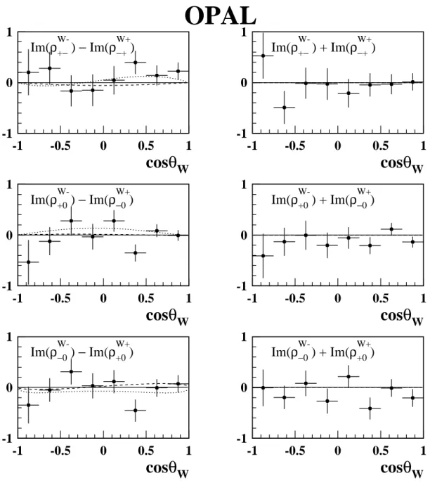
Im(ρ^W_τ1τ⁻₂) − Im(ρ^W−τ⁺1−τ2) = 0 (6) Thus CPT and CP-conservation together dictate that all coefficients fromρ^W_τ1τ2 are real. Deviations from the validity of equation (6) would represent an unambiguous signal for CP-violation at tree level.

Deviations from the equality of equation (5) represent a signal of higher-order (loop) effects beyond tree level [2].

The exclusive differential cross-sections for the production of a W with transverse (T) or longitu- dinal (L) helicity are obtained by weighting the total differential cross-section by the relevant elements of the single particle ρmatrix:

dσ_T

dcosθ_W = (ρ₊₊+ρ−−) dσ dcosθ_W dσ_L

dcosθW

= (ρ₀₀) dσ dcosθW

(7) and the corresponding total cross-sections are given by:

σ_T = Z +1

−1

(ρ₊₊+ρ−−) dσ dcosθW

dcosθ_W σL =

Z +1

−1

(ρ00) dσ

dcosθWdcosθW. (8)

The single W SDM elements can be obtained from measurements of the properties of the W decay products by the application of suitable projection operators Λ_{τ τ}^′ [1,2] which assume the V−A coupling of the W to fermions. The W decays are characterised by the polar and azimuthal angles of the decay fermion in the W rest frame,θ^∗andφ^∗respectively. In this analysis we consider only the semi-leptonic event class, WW→qqℓν, where one W decays to a lepton (e,µorτ) and a neutrino and the other to two hadronic jets. In this case the values ofθ^∗andφ^∗of the lepton may be determined unambiguously and the corresponding single W SDM elements are given by:

dσ(e⁺e⁻→W⁺W⁻) dcosθ_W ρ^W_{τ τ}⁻′

= 1

Br(W⁻→ℓ⁻¯ν)

Z dσ(e⁺e⁻→W⁺ℓ⁻ν)¯

dcosθ_Wdcosθ^∗dφ^∗ Λτ τ^′(θ^∗, φ^∗)dcosθ^∗dφ^∗ (9) In section 4 we describe how this expression is realised as a sum over the events observed in the data sample.

In the case of the hadronically decaying W differentiation between the particle and anti-particle decay products is very difficult. However, certain projection operators are symmetric under the trans- formation cosθ^∗→ −cosθ^∗,φ^∗ →φ^∗+π, i.e. the interchange of one of the decay particles from the W boson with the other decay particle, for example the u-type quark with the d-type in a hadronically decaying W boson. This means that a number of combinations of the SDM elements may still be extracted from W→ q¯q decays: these include ρ+++ρ⁻⁻ and ρ00. Both W bosons in the event can therefore be used to measure the polarised cross-section, since only these terms appear in equations (7).

Returning to the full two particle SDM, the analogous expressions to (7) but describing the dif- ferential cross-section for both W bosons in the pair being transversely polarised (TT), both being longitudinally polarised (LL), or one of each polarisation (TL) are:

dσ_TT

dcosθ_W = (ρ₊₊₊₊+ρ₊₊⁻⁻+ρ⁻⁻₊₊+ρ⁻⁻⁻⁻) dσ dcosθ_W dσ_LL

dcosθ_W = (ρ₀₀₀₀) dσ

dcosθ_W (10)

dσ_TL

dcosθ_W = (ρ₊₊₀₀+ρ−−00+ρ₀₀₊₊+ρ₀₀−−) dσ dcosθ_W

and the analogous expression to (9) is dσ(e⁺e⁻→W⁺W⁻)

dcosθ_W ρ_τ−τ′

−τ+τ₊^′

= 1

Br(W→qq)Br(W→ℓν)

Z dσ(e⁺e⁻→qqℓν)

dcosθWdcosθ−^∗dφ^∗−dcosθ^∗₊dφ^∗₊ (11)

× Λ_τ−τ−^′ (θ^∗−, φ^∗−)Λ_τ+τ^′₊(θ₊^∗, φ^∗₊)dcosθ−^∗dφ^∗−dcosθ^∗₊dφ^∗₊ where the integral is now over the decay angles of both W bosons.

3 The Data Sample and Monte Carlo Simulated Events

3.1 The Data Sample

The W-pair data used in this analysis were collected by the OPAL [18] detector at LEP. The accepted integrated luminosity in 1998, evaluated using small angle Bhabha scattering events observed in the silicon tungsten forward calorimeter [19], is 183.14 ± 0.55 pb⁻¹ [20]. The luminosity-weighted mean centre-of-mass energy for the data sample is√

s= 188.64±0.04 GeV.

In this analysis we use only the W-pair events decaying to the qqeν, qqµνand qqτ νchannels. These qqℓν events were first selected using the likelihood selection described in [9, 20, 21]. The selection is designed to optimise the rejection of Z⁰/γ→q¯q and four-fermion backgrounds. A total of 1252 qqℓν candidates was selected at this stage. Monte Carlo studies show this selection is about 88% efficient.

Further cuts are applied in order to obtain a sample of well reconstructed events. A full description can be found in [10]. A brief overview of the procedure is given here. For the qqeν and qqµν events a well reconstructed lepton track is required. For the qqτ ν events, either one track or a narrow jet consisting of three tracks is assigned as theτ decay product.

Kinematic fits are now applied to the events. For the qqeν and qqµν events a one-constraint fit is applied that requires energy-momentum conservation and neglects any initial state radiation. Events are accepted if the fit converges with a probability larger than 0.001. An improvement is made to the resolution of the angular observables by performing a second kinematic fit which constrains each reconstructed W mass to the average value measured at the Tevatron [22]. Events for which the fit converges with a probability of at least 0.001 are accepted; for other events we revert to the previous fit.

For the qqτ ν events a different kinematic fit is applied [9]; here the reconstructed mass of the two W bosons is required to be equal. In order to obtain a W mass from the leptonic part of these events, it is necessary to assume that the direction of the visible part of theτ decay approximates the direction of the τ lepton. The fit is required to converge with a probability of at least 0.025. This cut rejects 41% of the background. It also rejects about 14% of the signal events, but preferentially rejects events where the τ decay products are not correctly identified.

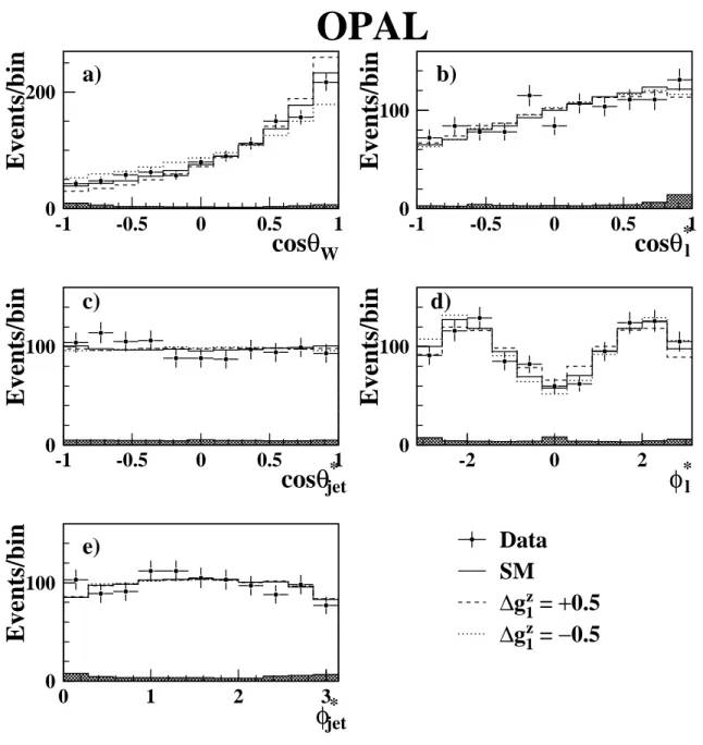
After application of all selection cuts 1065 qqℓν candidates remain, with 359 in the qqeν channel, 386 in the qqµν channel and 320 in the qqτ ν channel. The W production and decay angles for these events are shown in figure 1. The background contributions to the data sample are estimated using Monte Carlo samples. The resulting contaminations are expected to be four-fermion (non-CC03) 3.1%,

Z⁰/γ→q¯q 2.1%, two-photon (multiperipheral) 0.2% and CC03 four-fermion (WW→qqqq andℓνℓν) 0.5%.

3.2 Monte Carlo

A number of Monte Carlo models are used to provide estimates of efficiencies and backgrounds as well as the expected W-pair production and decay angular distributions for different TGC values.

The Monte Carlo samples are generated at √

s = 189 GeV. All Monte Carlo samples mentioned below are passed through the full OPAL simulation program [23] and then subjected to the same selection and reconstruction procedure as the data. The ERATO [13] Monte Carlo program is used in this analysis because it can generate samples of four-fermion Monte Carlo events with non-Standard Model values of CP-violating anomalous couplings. The EXCALIBUR [24] Monte Carlo is also used extensively in this analysis for correction of detector effects and as the main tool to compare to the 189 GeV data. A comparison between ERATO and EXCALIBUR angular distributions and spin density matrix elements was undertaken and no statistically significant differences were seen between them. The other four-fermion generator used to calculate background contributions and systematic uncertainties is grc4f [25]. The WW generators used to calculate theoretical predictions for the W-pair polarisations and to calculate systematic uncertainties are EXCALIBUR, HERWIG [26], PYTHIA [27]

and KORALW [28]. The background Z⁰/γ →q¯q samples are generated using PYTHIA. For samples of two-photon (multiperipheral) background PYTHIA, PHOJET [29] and HERWIG were used.

4 Measurement of W Boson Polarisation

4.1 Experimental Method

Measurements of the production cross-sections for each of the transverse and longitudinal states of the W bosons are obtained from summations of the SDM elements obtained from the qqℓν data sample, after correcting for detector acceptance, resolution effects and background contamination.

To calculate the SDM elements the events are divided into eight equal bins,k, of cosθ_W. In each bin the SDM elements are obtained by a summation over events, i, weighted by the relevant SDM projection operators as shown in equation (12). This is effectively the realisation of equation (9) as a summation over observed events. Nk is the number of events in bin k. In the extraction of all the individual W SDM elements CPT invariance is assumed, so all leptonic (hadronic) W⁺ and W⁻ decays can be combined.

ρ^k_{τ τ}′(cosθ_W^k ) = 1 N_k

Nk

X

i=1

Λ_{τ τ}^′(cosθ_i^∗, φ^∗_i) (12) Estimates of the production cross-sections are derived from the diagonal SDM elements; therefore the projection operators only involve the polar decay angle cosθ^∗. It is not required that the SDM elements be positive definite. Both the leptonic and hadronic W decays can be used since the SDM combinations occurring in equation (7) are symmetric with respect to the use of the fermion or anti- fermion polar decay angle. Each event is also weighted by a correction factor,f, for detector acceptance and resolution effects:

ρ^k₀₀= 1 N_k^cor

Nk

X

i=1

1

f_k(θ_i^∗)Λ₀₀(θ_i^∗) (13)

ρ^k₊₊+ρ^k−− = 1 N_k^cor

Nk

X

i=1

1

fk(θ^∗_i)(Λ₊₊(θ^∗_i) + Λ⁻⁻(θ^∗_i)) (14) whereN_k^cor is the corrected number of events in bin k:

N_k^cor=

Nk

X

i=1

1

f_k(θ_i^∗). (15)

The factors f_k(θ_i^∗) are obtained from fully simulated Monte Carlo events, and are calculated as a function of cosθ_W and cosθ^∗. They are defined to be the ratio of the number of reconstructed events to the number of generated events in each bin. The correction factors have an effect of between 5%

and 20%. The typical resolution of the measured cosθ_W is found to be 0.05, which is less than 20%

of the bin width used in correcting this distribution. The typical resolution of the measured cosθ^∗ is found to be 0.07, which is 70% of the bin width used in the calculation of the correction factors.

The distribution of uncorrected events, shown in figure 1, also has to be corrected for detector acceptance and resolution effects. This is done in a similar manner to the correction of the SDM elements by calculating a correction factor from Monte Carlo events in a bin-wise fashion and applying it to the data. The estimated background contribution is subtracted from the SDM elements and the dσ/dcosθ_W distribution.

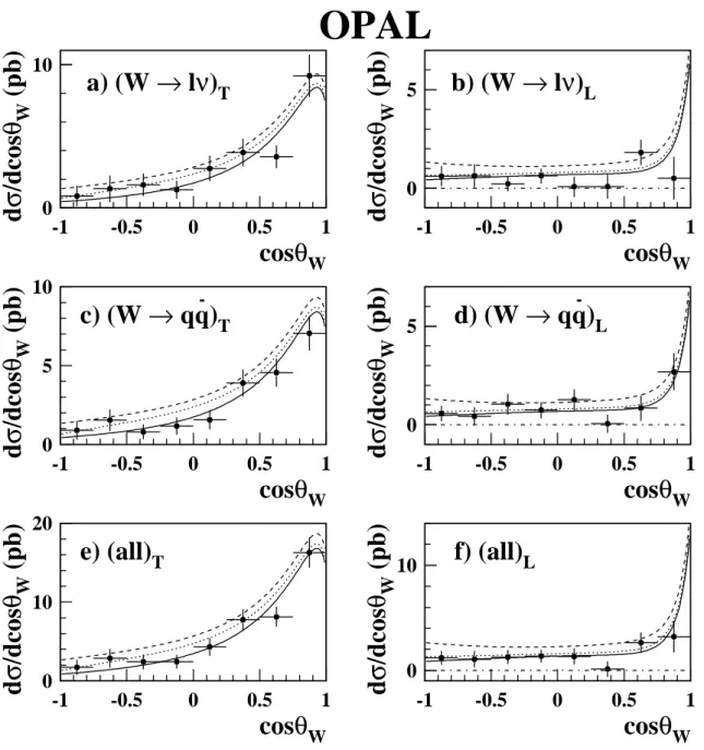
The polarised differential cross-sections, dσL/dcosθW and dσT/dcosθW, are then obtained by mul- tiplying the binned unpolarised differential cross-section by the relevant SDM combinations, following equations (7).

4.2 Experimental Results

Figure 2 shows the individual W boson differential cross-sections obtained from the data by this method. The transverse and longitudinal components obtained from the leptonically decaying W and the hadronically decaying W are shown separately, together with the values obtained by combining the two. The polarisations of the W bosons in the W-pair event are correlated. The correlation is estimated to be 0.07, and is taken into account in the errors on the combined cross-sections.

The fraction of each polarisation state, obtained by integrating over cosθW and then dividing by the total cross-section, is given in table 1. Once again the correlated polarisations of the two W bosons are taken into account when deriving the errors. The estimation of the systematic errors shown in tables 1 and 2 is described in section 6.

The joint polarised cross-sections are obtained by extracting the joint SDM elements in a similar way to equations (12)

ρ^k_τ

−τ₋^′τ+τ₊^′ = 1 N_k^cor

Nk

X

i=1

1

fk(θ_i^∗lept, θ^∗_i^had)Λ^W_τ−^±_τ′−(θ^∗_i^lept)Λ^W_τ+^∓_τ′+(θ^∗_i^had) (16) where in this case theρ and Λ are those corresponding to the particular SDM combinations appearing in equation (10). Note that there is now a projection operator for each W, and the correction factor is binned in terms of both polar decay angles. Figure 3 shows the joint differential cross-sections obtained by this method, these cross-sections are not constrained to be positive definite.

The fractions of each helicity state, obtained by integrating over cosθ_Wof the W and then dividing by the total cross-section, are shown in table 2. These results are highly correlated. The correlations

σ_T/σ_total σ_L/σ_total Data

W→ℓν 0.842 ±0.048 ±0.023 0.158 ±0.048 ±0.023 W→qq 0.738 ±0.045 ±0.025 0.262 ±0.045 ±0.025

All 0.790 ±0.033 ±0.016 0.210 ±0.033 ±0.016

Standard Model Expectation

W→ℓν 0.746± 0.006 0.254± 0.006

W→qq 0.741± 0.006 0.259± 0.006

All 0.743± 0.004 0.257± 0.004

Table 1: The fractions of transversely and longitudinally polarised W bosons. The expected values are from generator level EXCALIBUR Monte Carlo, the errors being statistical only. The first error on the measured values is statistical and the second is the systematic uncertainty.

between each helicity fraction, calculated from the data, are found to be: σ_TT:σ_LL = 0.67±0.02, σ_TT:σ_TL =−0.93±0.01 and σ_LL:σ_TL =−0.89±0.01.

The individual W polarised differential cross-sections show good agreement with the Standard Model predictions, as do the overall fraction of each individual W polarisation, as seen in table 1.

The W pair polarised cross-sections show less good agreement, but σLL/σ_total is within two standard deviations of the Standard Model prediction and the other two are just over two standard deviations away. The χ² value for the three measurements compared to the Standard Model expectations, including systematic uncertainties, is 4.7. This corresponds to aχ² probability of 10%.

Measured Expected

σ_TT/σ_total 0.781 ±0.090 ±0.033 0.572 ±0.010 σ_LL/σ_total 0.201 ±0.072 ±0.018 0.086 ±0.008 σ_TL/σ_total 0.018 ±0.147 ±0.038 0.342 ±0.016

Table 2: The fraction of each helicity combination of WW pairs. The expected values are calculated from Monte Carlo studies. The first errors on the measured fractions are statistical and the second are systematic. The errors on the expected fractions are statistical only.

5 Measurement of Anomalous Couplings and Test of CP-Invariance

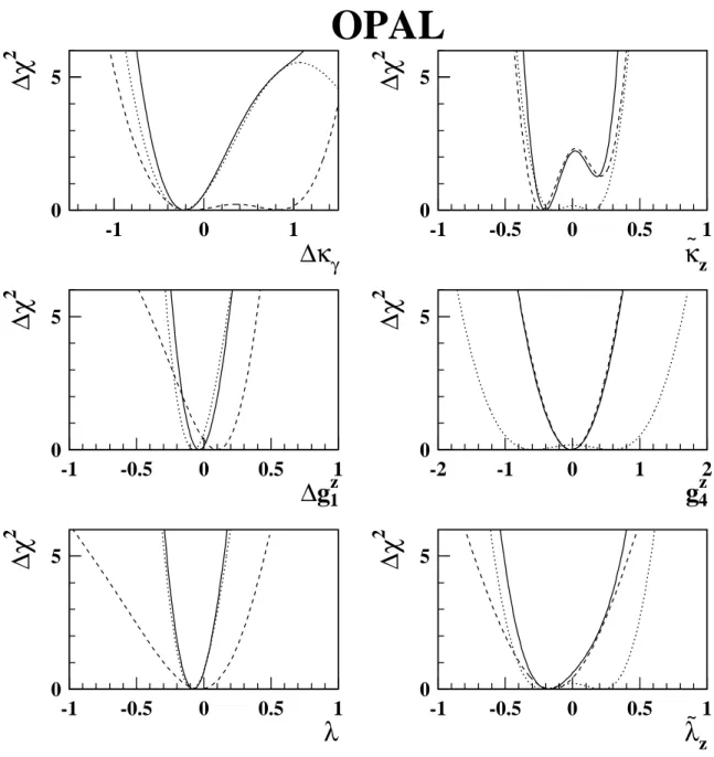
Measurements of anomalous coupling parameters are obtained through a comparison of distributions of SDM elements obtained from the leptonically decaying W bosons in the qqℓν data sample with distributions obtained from fully simulated Monte Carlo samples. In contrast to the polarised cross- section measurements, neither data nor Monte Carlo events are corrected for detector or acceptance effects. Instead the experimentally observed SDM distributions are compared directly with those for fully detector simulated Monte Carlo events. Monte Carlo samples for arbitrary TGC values are obtained by a re-weighting technique applied to a large Standard Model sample. A χ² minimisation procedure is then used to find the simulated data set which best fits the data and hence obtain the best fit TGC parameter value.

The events are again divided into eight equal bins of cosθ_W. Equation (12) is used to calculate all six real and three imaginary SDM elements directly. The SDM distributions are shown in figure 4.

This method is used to calculate both the CP-conserving and the CP-violating couplings. However,