The FluxEngine air–sea gas flux toolbox: simplified interface and extensions for in situ analyses and multiple sparingly soluble gases

(1)

https://doi.org/10.5194/os-15-1707-2019

The FluxEngine air–sea gas flux toolbox: simplified interface and extensions for in situ analyses and multiple sparingly soluble gases

Thomas Holding¹, Ian G. Ashton¹, Jamie D. Shutler¹, Peter E. Land², Philip D. Nightingale², Andrew P. Rees², Ian Brown², Jean-Francois Piolle³, Annette Kock⁴, Hermann W. Bange⁴, David K. Woolf⁵,

Lonneke Goddijn-Murphy⁶, Ryan Pereira⁷, Frederic Paul³, Fanny Girard-Ardhuin³, Bertrand Chapron³, Gregor Rehder⁸, Fabrice Ardhuin³, and Craig J. Donlon⁹

1University of Exeter, Penryn Campus, Cornwall, TR10 9EZ, UK

2Plymouth Marine Laboratory, Prospect Place, Plymouth, PL1 3DH, UK

3Ifremer, Univ. Brest, CNRS, IRD, Laboratoire d’Oceanographie Physique et Spatiale (LOPS), IUEM, Brest, France

4GEOMAR Helmholtz Centre for Ocean Research Kiel, Marine Biogeochemistry Research Division, 24105 Kiel, Germany

5International Centre for Island Technology, Heriot-Watt University, Stromness, Orkney, KW16 3AW, UK

6Environmental Research Institute, University of the Highlands and Islands, Thurso, KW14 7EE, UK

7The Lyell Centre, Heriot-Watt University, Research Avenue South, Edinburgh, EH14 4AS, UK

8Leibniz Institute for Baltic Sea Research Warnemünde, 18119 Rostock, Germany

9European Space Agency, Noordwijk, the Netherlands

Correspondence:Thomas Holding (t.m.holding@exeter.ac.uk) Received: 1 May 2019 – Discussion started: 15 May 2019

Revised: 5 November 2019 – Accepted: 7 November 2019 – Published: 13 December 2019

Abstract. The flow (flux) of climate-critical gases, such as carbon dioxide (CO2), between the ocean and the atmosphere is a fundamental component of our climate and an important driver of the biogeochemical systems within the oceans.

Therefore, the accurate calculation of these air–sea gas fluxes is critical if we are to monitor the oceans and assess the impact that these gases are having on Earth’s climate and ecosystems. FluxEngine is an open-source software toolbox that allows users to easily perform calculations of air–sea gas fluxes from model, in situ, and Earth observation data. The original development and verification of the toolbox was described in a previous publication. The toolbox has now been considerably updated to allow for its use as a Python library, to enable simplified installation, to ensure verification of its installation, to enable the handling of multiple sparingly soluble gases, and to enable the greatly expanded functionality for supporting in situ dataset analyses. This new functionality for supporting in situ analyses includes user-defined grids, time periods and projections, the ability to reanalyse in situ CO₂ data to a common temperature dataset, and the ability to easily calculate gas fluxes using in situ data from drifting buoys, fixed moorings, and research cruises. Here we

describe these new capabilities and demonstrate their application through illustrative case studies. The first case study demonstrates the workflow for accurately calculating CO₂ fluxes using in situ data from four research cruises from the Surface Ocean CO₂ ATlas (SOCAT) database. The second case study calculates air–sea CO₂ fluxes using in situ data from a fixed monitoring station in the Baltic Sea. The third case study focuses on nitrous oxide (N₂O) and, through a user-defined gas transfer parameterisation, identifies that biological surfactants in the North Atlantic could suppress individual N₂O sea–air gas fluxes by up to 13 %. The fourth and final case study illustrates how a dissipation-based gas transfer parameterisation can be implemented and used. The updated version of the toolbox (version 3) and all documentation is now freely available.

1 Introduction

The exchange of climate relevant gases between the oceans and atmosphere including that of carbon dioxide (CO₂), nitrous oxide (N₂O), and methane (CH₄) is a major component

(2)

of the climate system, and the ability of the oceans to ab- sorb and desorb these gases varies both temporally and spatially. The need to monitor this exchange has been the driver for international data collation initiatives such as the Surface Ocean CO₂ATlas (SOCAT; Bakker et al., 2016) and the Ma- rinE MethanE and NiTrous Oxide database (MEMENTO;

Kock and Bange, 2015). These collaborative efforts are now routinely collecting, quality controlling and collating over a million new in situ data points each year. FluxEngine com- plements these initiatives by providing a standardised tool which can robustly calculate air–sea gas fluxes from such in situ data, with the flexibility to incorporate new data sources and methodologies. The use of common tools and methods simplifies collaborations and accelerates advancements, both within and between scientific disciplines, through elimi- nating methodological or implementation-driven differences and the duplication of effort.

1.1 Overview of FluxEngine

FluxEngine is a flexible open-source toolbox that allows users to easily exploit Earth observation and model data, in combination with in situ data, to calculate air–sea gas fluxes (Shutler et al., 2016). It is available to download from http://github.com/oceanflux-ghg/FluxEngine (last access: 6 December 2019). The toolbox uses plain-text configuration files, allowing the user to configure the input data sources, random noise or bias on input data, the temporal period for the analysis, the structure of the air–sea gas flux calculation, and user-defined gas transfer velocity parameterisations. The calculation itself can be performed using fugacity, partial pressure, or concentration data via a user-defined bulk formulation, including formulations that can account for vertical temperature gradients across the mass boundary layer, the very small layer at the surface over which gas exchange occurs. A full description of the differences between flux formulations is provided in Shutler et al. (2016) and Woolf et al. (2016). The formulation that enables vertical temperature and salinity gradients to be included, allowing a more accurate gas flux calculation is described in detail by Woolf et al. (2016) and takes the generalised form of

F =k(α_Wf G_W−α_Sf G_A), (1) where F is the sea-to-air flux of a sparingly soluble gas G,k is the gas transfer velocity, αS and αW are the solubilities of the gas above and below the surface water interface, andf GAandf GWrepresent the respective fugacities.

Here we use “p” and “f” prefixes to refer to partial pressure and fugacity of a gas, respectively. Gas transfer velocity is driven by turbulence at ocean surface, caused by wind stress and wave breaking, amongst other processes. Because of the wide availability of high-quality wind data products and the relative difficulty of directly measuring turbulence, it is com- monplace to estimate kusing a statistical relationship with

wind speed (e.g. Ho et al., 2006; Nightingale et al., 2000;

Wanninkhof, 2014).

Concentration of the gas is determined by its solubility and fugacity (or partial pressure). Equation (1) can therefore be rewritten as a product of the gas transfer velocity and the difference in gas concentrations,

F =k(G_W−G_S), (2)

whereG_SandG_Ware the concentration of the gas above and below the interface. The FluxEngine configuration file allows users to choose the structure of the gas flux calculation, the inputs, and the gas transfer velocity (either by choosing an already implemented published algorithm or through param- eterising their own). The user can then perform calculations across their chosen input data and the outputs are Climate and Forecast (CF) standard netCDF 4.0 files that contain data layers for each of the stages of the calculation, along with process indicator layers to aid the interpretation of the calculated gas fluxes (such as surface chlorophyllaconcentrations, the climatological position of temperature fronts, and error indicator layers). A summary of the main features of the toolbox is given in Table C1 (Appendix C).

Version 1.0 of FluxEngine was introduced and described by Shutler et al. (2016), which included a full description of the calculations, the flexibility of the toolbox, and the extensive verification of the different calculations along with examples of its use. With the aim to provide a standardised community tool, development has continued since its original release. Feedback from the user communities and the needs of specific scientific studies (e.g. Ashton et al., 2016) have guided these developments and considerably extended the functionality and range of possible applications.

At the time of writing, the toolbox and resulting data have been used to quantify regional and global uncertainties (e.g.

Wrobel and Piskozub, 2016; Wrobel, 2017; Woolf et al., 2019; Shutler et al., 2019), evaluate the impact of gas transfer processes on regional and global gas exchange (e.g. Ashton et al., 2016; Pereira et al., 2018), evaluate the European shelf sea CO₂gas fluxes and sinks (Shutler et al., 2016) and investigate biological and physical controls of air–sea exchange (Henson et al., 2018). FluxEngine has also been used to identify shortfalls of current modelling approaches through the inclusion of FluxEngine outputs within an international inter-comparison (Rödenbeck et al., 2015). The toolbox has also been incorporated within undergraduate and postgrad- uate teaching at the University of Exeter within geography, environmental science, and marine biology degrees, and at Utrecht University for computer science.

This paper uses four case studies to illustrate key developments and the extended capabilities now contained within version 3.0 of the FluxEngine toolbox. Collectively, the case studies illustrate user-selectable grids, support for calculating sea-to-air gas fluxes from time series data collected by fixed monitoring stations and research cruises (and how to incorporate the flux outputs into the original dataset to create

(3)

a coherent time series), the ability to calculate nitrous oxide (N₂O) sea-to-air gas fluxes, and the addition of a new forcing variable (kinetic energy dissipation rate). The extensive support for in situ data contained within version 3 of Flux- Engine means that it can now be fully exploited by three different scientific communities in isolation: in situ, model, and Earth observation, whilst the original capability to enable gas fluxes to be calculated from combinations of in situ, model, and Earth observation data is retained.

Section 2 of this paper describes the structural extensions and changes and explains how the toolbox can now be used as a command-line tool or as a Python library. Section 3 then presents the case studies, and Sect. 4 outlines the future direction and developments for the toolbox; Sect. 5 gives conclusions. To aid the user, the appendices of this paper provide a list all of the toolbox utilities (Appendix A), details of all datasets used in the case studies (Appendix B), an overview of the main toolbox features and options (Appendix C), and a description of the automatic software installers and verification tools (Appendix D).

2 New capabilities

The following sections describe the extensions to the Flux- Engine toolbox that are now contained within version 3.

2.1 Installation, verification, and use

FluxEngine has now been optimised for use on a stand-alone desktop or laptop computer, removing the previous require- ment for specialist computing facilities. Installation tools or instructions are provided for Microsoft Windows, Apple MacOS, and Ubuntu/Debian-based Linux operating systems.

Separate utilities can then be used to verify that FluxEngine has been successfully installed. Details of the installation, verification process, and execution times are provided in Ap- pendix D.

FluxEngine is now implemented as a Python module, which means that FluxEngine and its accompanying utilities can be imported as a Python module and easily integrated with other software or use as stand-alone tools that are called from the command line. This approach offers a larger degree of flexibility than offered by version 1 of the toolbox and supports advanced exploitation. For example, a simple Python script can be written to run a sensitivity analysis where en- sembles of flux calculations are required without any need to modify the underlying FluxEngine software.

2.2 Flexible input data specification

Previous versions of FluxEngine required the user to make changes to the underlying software in order to use new or differently formatted sources of input data. This required additional (and time consuming) testing and verification after modifications were made, making FluxEngine less accessi-

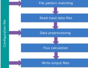
Figure 1.Conceptual diagram showing the way that input data are imported and used by FluxEngine. Single or groups of files are specified using a plain-text configuration file. File names are interpreted using a subset of regular expression matching syntax (Unix glob patterns), and additional tokens are used to substitute time and date.

The data preprocessing steps occur after input files are read into memory. Preprocessing functions are specified in the configuration file. Finally, the netCDF output files follow a user-specified file- name and directory structure (as specified in the configuration file).

ble to those unfamiliar to Python programming. Two features have been added in version 3.0 to address this issue:

(i) file pattern matching (through standard Unix glob patterns and custom date/time tokens, described fully inFlux- EngineV3_instructions.pdf) allows the input file name format and directory structure to be customised using the plain-text configuration file, and (ii) optional preprocessing functions can be used to manipulate input data after the data have been read into memory. These features can be specified for each input variable in the configuration file and FluxEngine contains a selection of common preprocessing functions, such as unit conversions or matrix transformation of the input data.

Additional custom preprocessing functions can be added and tested easily by the user without the need to modify the core FluxEngine software, through copying and then completing the Python template function provided within the source code (data_preprocessing.py). Storing the completed function into thedata_preprocessing.pyfile will then result in the custom preprocessing function being automatically available for use in any configuration file.

These features make it possible to use any observational netCDF dataset by specifying the file path and, if required, appropriate preprocessing functions. For example a custom preprocessing function could resample the input files, fol- lowed by a transformation to change the projection. This flexibility is conceptualised by the diagram in Fig. 1.

(4)

2.3 Extensive support for in situ data analyses

Version 1 of FluxEngine required that all input data be sup- plied as monthly 1^◦×1^◦ global grids. These constraints re- stricted its relevance to regional analyses and in situ analyses, where sub-daily or sub-kilometre resolutions are often more appropriate. The spatial resolution and extent can now be fully specified by the user and regional masks can be used in conjunction with theofluxghg_flux_budgets.pytool to calculate regional net integrated fluxes. In addition, flexible start and stop times and user-specified temporal resolutions allow gas fluxes to be calculated for specific time intervals, e.g. the calculation can be configured to match the temporal resolution of the in situ data. Furthermore, a new configuration option allows the output from multiple time points to be grouped into a single netCDF file (rather than multiple files, one for each time point). This enables the calculation of gas fluxes from fixed research stations and other scenarios in which it is more convenient to provide results as a time series.

Improvements have been made to the bundled file conversion utilities, which convert between plain-text data formats and the netCDF format used by FluxEngine. By de- fault, these tools use the SOCAT format (Bakker et al., 2016) for convenience but now offer a high degree of flexibility to reflect the variety of data formats and conventions used for storing in situ data. This means that the tools can be used with virtually any text-formatted in situ data files, avoiding the need for the user to convert their data to a fixed format with predefined column names.

The new utility,append2insitu.py, is designed specifically for use with in situ data and appends FluxEngine output as new columns within the original in situ data (achieved by matching spatial and temporal coordinates). For example, this means that users can use SOCAT-formatted (or custom- formatted) in situ data as input to FluxEngine and then the results can be placed into a copy of the original input file, allowing the user to study the calculated fluxes, gas transfer rates, gas concentrations, etc. alongside (and aligned with) their original in situ data. This functionality is demonstrated in case study 1 and case study 3 within this paper.

2.4 Reanalysis of in situ CO₂fugacity data to a consistent temperature and depth

A new utility, reanalyse_socat_driver.py, is CO2 specific and exploits a reference (sea surface temperature) SST dataset (e.g. climate quality Earth observation SST data) and the original paired in situ measurements of CO₂ fugacity (fCO₂) and temperature to recalculate thefCO₂for the reference temperature dataset (and thus a consistent depth). The reasoning for the reanalysis is to reduce uncertainty and unknown biases that arise due to thefCO₂measurements being collected using different instrumentation at some unknown and potentially variable depth below the surface. A detailed

justification of the method and a full description of the approach are described in Goddijn-Murphy et al. (2015).

The reanalysis step is especially important if in situ data consisting of a collated dataset (originating from different instruments, sampling strategies, or sources) is being used to calculate temporally averaged gas fluxes (e.g. monthly mean values). In this situation the in situ measurements are highly likely to be collected from a range of different depths and unlikely to fully capture the monthly mean conditions of temperature andfCO₂(due to aliasing), whereas temporally averaged (mean) satellite observations are likely to provide a better representation (reference) of the mean temperature conditions. Therefore reanalysing the collatedfCO2dataset to this reference temperature enables the calculation of the equivalent meanfCO2data.

It is worth noting that ship draught, and thus underway measurement intake depth, can even vary on a single research cruise due to changes in sea state, ballasting, or cargo. So the method can also be important for data collected during a single research cruise.

For the case studies presented here, the satellite-observed SST data used for the reanalysis are valid for a depth of

∼1 m (Reynolds et al., 2007). So the recalculatedfCO₂data are therefore also valid for this depth and are used to represent the conditions at the bottom of the mass boundary layer or sub-skin temperature. The reanalysis to a consistent depth also enables a more accurate calculation of the gas fluxes, as it is then possible to accurately calculate two solubilities and thus two concentrations: one at the bottom and one at the top of the mass boundary layer.

The Goddijn-Murphy et al. (2015) reanalysis method re- lies upon variations infCO₂being purely isochemical. This assumes that the total dissolved inorganic carbon is approximately constant throughout the surface waters over the temporal period and spatial scale being studied and that differences infCO₂are solely due to temperature differences altering the equilibria of the carbonate system. Therefore cau- tion should be used when applying the reanalysis method to data where these assumptions are not valid.

The slow re-equilibrium time of CO₂in seawater (i.e. of the order of months for CO₂ to equilibrate with the atmosphere) ensures that monthly mean, or rolling monthly mean (centred on the day of interest), skin or sub-skin sea surface temperature (SST) values are suitable for reanalysing the in situ data. Arguably, for reanalysing individual in situ datasets (e.g. to calculate gas fluxes for a single cruise dataset) a ro- bust daily skin or sub-skin SST value would be better, even if that is obtained by a seasonal curve fitted to the monthly values and interpolated to the day of interest. Another solution would be to collect paired measurements of skin SST and fCO₂and SST at depth, all in situ, as has been done on a re- cent research cruise (Tarran, 2018) as ship-ready instruments are available, e.g. the Infrared Sea surface Autonomous Ra- diometer (ISAR; Donlon et al., 2008). This enables the paired measurements at depth to be reanalysed using the in situ

(5)

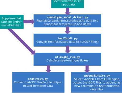
Figure 2.A typical CO₂workflow for using FluxEngine with in situ data, showing the different utilities (blue boxes) and input data (green boxes) used at each stage.

skin SST. However in the majority of cases ships collecting fCO₂ data do not collect skin temperature data. Where in situ skin temperature data are not available and satellite temperature data are not appropriate, a regional model could be used to estimate skin temperature from the SST a few metres below the surface. An example model capable of this is the US National Oceanic and Atmospheric Administration (NOAA) Coupled Ocean–Atmosphere Response Experiment (COARE) model (e.g. see Fairall et al., 1996).

Whilst the reanalysis method and utility is CO₂specific, its applicability to alternative gases (including unreactive N₂O and CH₄) is discussed and shown in Table 1 of Woolf et al. (2016). The impact on the net gas fluxes of not performing this reanalysis on a relatively large time series of CO₂measurements through the north and south Atlantic is demonstrated within case study 1 (Sect. 3.1), whereas the impact on global net integrated gas fluxes has been analysed by Woolf et al. (2019).

A typical workflow for calculating sea-to-air gas fluxes from in situ data using FluxEngine, and the tools used at each step, is illustrated in Fig. 2. All of the in situ analysis utilities, including the use of thereanalyse_socat_driver.pytool, are demonstrated in case study 1 to case study 3 (Sect. 3).

2.5 Custom gas transfer velocity parameterisation The processes that govern exchange, their relative impor- tance, and how gas exchange should be parameterised are

all active areas of research (e.g. Pereira et al., 2018; Wrobel and Piskozub, 2016).

FluxEngine has always allowed users to select or define different gas transfer velocity parameterisations. However, version 3.0 adopts a modular approach to specifying the flux calculation, which makes it simpler for the user to extend the functionality and incorporate new gas transfer parameterisations. Custom parameterisations can be implemented as separate Python classes without modifying the core Flux- Engine software. This is achieved by copying and modifying the template class provided inrate_parameterisation.py.

Storing the new class withinrate_parameterisation.pymeans that the new parameterisation will be automatically available for inclusion in the configuration file. These custom parameterisations can define new input variables and therefore make use of additional input data sources. These custom parameterisations can also produce new data layers in the final netCDF output, such as the results from intermediate calculation steps, which may be useful for testing or subsequent analysis outside of FluxEngine. Examples of how to use this functionality are provided in the source code. The toolbox documentation describes the process of, and best practices for, extending FluxEngine in this way (see Sect. 9.1 and 9.2 withinFluxEngineV3_instructions.pdf).

This increased flexibility means that users can define and use region-specific gas transfer parameterisations or incorporate new transfer processes into existing gas transfer parameterisations (such as the impact of biological surfactants as

(6)

discussed by Pereira et al. (2018). Case study 1 (Sect. 3.1) and case study 2 (Sect. 3.2) demonstrate the use of different well-known wind-speed-based gas transfer parameterisations, while case study 3 (Sect. 3.3) demonstrates the use of a custom gas transfer velocity parameterisation, which is used to assess the impact of biological surfactants on the N₂O gas fluxes. Case study 4 (Sect. 3.4) utilises a gas transfer velocity parameterisation that is based on turbulent kinetic energy dissipation and provides an example of using additional input data.

2.6 Extensions for other sparingly soluble gases The toolbox now supports the handling of two other sparingly soluble gases (CH₄and N₂O) and so that gas-specific data can be substituted into Eqs. (1) or (2) (dependent upon the choice of setup). FluxEngine can calculate dissolved gas concentration from these gas input data, which can be sup- plied as either partial pressure or mean molar fraction of a gas in the dry atmosphere. Alternatively, dissolved gas concentrations can be provided directly as an input. Gas-specific parameterisations for Schmidt number (Sc) and solubility (α) are automatically chosen from those provided in Wan- ninkhof (2014). The option to use the older Sc andα parameterisations from Wanninkhof (1992) is also included for compatibility with previous versions and to aid comparative analysis. It is worth noting that both sets of Scparameter- isations are only valid for saline water, and care should be taken when using them for analysis of freshwater data or regions with low salinity (e.g. the Baltic Sea; see case study 2, Sect. 3.2). Support for additional and user-defined Schmidt number parameterisations are likely to be added in the future.

3 Case study examples of the new capabilities

The following sections describe the application and results from four case studies that illustrate the new capabilities.

Table 1 summarises the new features that are demonstrated in each case study. These case studies were run using Flux- Engine version 3.0, which can be accessed via the GitHub repository (see “Code availability”). The configuration files for each case study are included as examples in the con- figs subdirectory of the GitHub repository, and these will be updated to maintain compatibility as new versions of the toolbox are released. In addition, interactive iPython Jupyter Notebook tutorials for the first three case studies are included in the tutorialssubdirectory of the repository. Section 4 of this paper provides more information about these tutorials.

3.1 Case study 1: calculating CO₂fluxes from research cruise data

Each year over 1 million new in situ data points are included within the annual updates to the SOCAT dataset. Field scien-

tists collecting these data often need to calculate the coincident sea-to-air gas fluxes, either using solely in situ measurements or through combining them with satellite Earth observation and/or model data.

Here we illustrate the procedure for calculating sea-to-air gas fluxes from in situ data collected during four different sampling campaigns. These in situ data (Kitidis and Brown, 2017; Schuster, 2016; Steinhoff et al., 2016; Wanninkhof and Pierrot, 2016; hereafter referred to as cruises 1–4, respectively) were all collected in the North Atlantic during Octo- ber 2013. The in situ data were first downloaded from PAN- GAEA (an open-access data publishing and archiving repository, http://www.pangaea.de, last access: 6 December 2019) in tab-delimited format. The datasets follow the standard SO- CAT structure and content (see Bakker et al., 2016, Table 9).

The majority of the measurements needed for the sea- to-air CO₂ gas flux calculation were included within the downloaded datasets. The aqueousfCO₂, salinity, SST, and air pressure were measured in situ and the molar fraction of CO₂ in dry air (xCO₂) had been extracted from the GLOBALVIEW-CO2 dataset (GLOBALVIEW-CO2, 2013).

However, wind speed (needed for calculating the gas transfer velocity) was missing in all cases. Therefore, to comple- ment these in situ data, multi-sensor merged wind speed data at 10 m were downloaded (Cross-Calibrated Multi-Platform, CCMPv2, 6 h temporal resolution, 0.25^◦×0.25^◦spatial grid;

Atlas et al., 2011). These wind speed data were appended to the in situ data by matching each in situ measurement to the closest temporal and spatial grid point. This same process was used to add columns for the second and third moments of wind speed, which were estimated by taking the second and third power of wind speed, respectively.

Two datasets (Schuster, 2016; Steinhoff et al., 2016) were missing xCO₂ data, so the same method of matching temporal and spatial grid points was used to fill in these fields using the GLOBALVIEW-CO2 dataset from the US National Oceanic and Atmospheric Administra- tion (NOAA) Earth System Research Laboratory (ESRL) (GLOBALVIEW-CO2, 2013). For ease, these additional wind speed andxCO₂data were downloaded, extracted, and then inserted into the tab-delimited in situ file using some simple custom Python scripts but the same process could be performed manually. These scripts are not part of Flux- Engine.

Collectively the in situ data from these cruises were collected from different ships and underway systems, all sampling water at different and unknown depths. These measurements are typically collected from a few metres below the water surface, whereas the CO₂concentration (combination offCO₂and solubility) on either side of the mass boundary layer is required for an accurate gas flux calculation. Before these data from multiple sources can be used for an accurate gas flux calculation, they need to be reanalysed to a common temperature dataset and depth (Goddijn-Murphy et al., 2015;

Woolf et al., 2016). Therefore, thereanalyse_socat_driver.py

(7)

Table 1.Summary of the new functionality demonstrated in each case study.

New features utilised Case study 1: calculating sea-to-air

CO₂ gas fluxes from ship research cruise data and using SOCAT data.

Flexible input data specification to select in situ data files and unit conversion using preprocessing functions (Sect. 2.2).

Utilises new support for in situ data analysis, including the use of thetext2ncdf.pyand append2insitu.pytools, custom temporal resolution, and reanalysis offCO₂to a consistent temperature field.

Case study 2: calculating sea-to-air CO₂ gas fluxes from the Östergar- nsholm fixed monitoring station data.

Flexible input data specification to select in situ data files and unit conversion using preprocessing functions (Sect. 2.2).

Utilises new support for in situ data analysis, including use oftext2ncdf.py, daily temporal resolution and output formatted as time series (Sect. 2.3).

Case study 3: surfactant suppression of sea-to-air N₂O gas fluxes using the ME- MENTO data.

Flexible input data specification and unit conversion using preprocessing functions (Sect. 2.2).

Utilises new support for in situ data analysis, including use of thetext2netcdf.pyand append2insit.py tools, custom temporal resolution, and cruise-specific time interval (Sect. 2.3).

Custom gas transfer parameterisation (Sect. 2.5).

Calculation of N₂O gas fluxes (Sect. 2.6).

Case study 4: gas transfer velocity parameterisation using turbulent kinetic energy dissipation rate.

Unit conversion and use of custom preprocessing functions to calculate the dissipation rate from the input data. This uses the preprocessing functions to perform a nontrivial computation (Sect. 2.2).

Use of a custom gas transfer parameterisation which includes the specification of an additional input data layer (Sect. 2.5).

tool was first used to reanalyse allfCO₂data to a consistent temperature and depth.

Monthly mean sea surface temperatures from the Reynolds Optimum Interpolation Sea Surface Temperature dataset (OISST; Reynolds et al., 2007) were used as the reference sub-skin temperature dataset, resulting in reanalysed fCO₂that are valid for∼1 m and used to represent the bottom of the mass boundary layer (termed “sub-skin” within Woolf et al., 2016).

The reanalysedfCO2data were then inserted into the tab- delimited in situ dataset producing a single dataset. The tab- delimited file was then converted into a netCDF file using the text2ncdf.pytool. This tool groups all data according to a user-specified spatial sampling grid, calculating the mean value and standard deviation for each cell within the grid as well as the number of data that were used to calculate these statistics. The spatial resolution was defined as 1^◦×1^◦grid and FluxEngine was then configured to use each of the variables in the resulting netCDF file as input, with a preprocessing function applied to convert Reynolds OISST from degrees Celsius to kelvin (as all SST data within the main flux calculation use kelvin). In order to produce a single netCDF output file for the entire 35 d period, the temporal resolution for the flux calculation was set to 35 d. This allows the cruise tracks from all four cruises (1–4) to be easily visualised at the same time.

The sea-to-air CO2 fluxes were then calculated using the rapid model (see Eq. (1) and Woolf et al., 2016) and was run

using a quadratic wind speed based gas transfer velocity parameterisation (Ho et al., 2007). To identify the impact of the fCO₂ reanalysis stage, the sea-to-air CO₂ flux calculation was repeated using the original in situ SST andfCO₂.

Figure 3a shows the resultant calculated CO₂flux along each of the cruises (1–4). The southern subtropical part of the cruise track 1 represents an area of the ocean that is a sink of CO₂(negative sea-to-air flux). The northern subtropical section of cruise 1 shows an overall positive CO2flux into the atmosphere, while south of 15^◦N the net fluxes are smaller and in variable directions. Interestingly, there are also examples (e.g. along the equatorial part of cruise track 1 and the west- ern part of cruise track 2) where the direction of the flux has changed as a result of reanalysing thefCO₂data. The high- est magnitude fluxes were seen around the European conti- nental shelf in cruise track 3, with a strong ocean sink west of Ireland and an intermittent source of CO₂ in the North Sea. Figure 3b shows the difference in calculated net flux between use of the originalfCO₂data and the reanalysed fCO₂. Whilst very little difference is seen over large lengths of cruise tracks 1, 2, and 4, there are substantial differences in net flux of up to 0.1C m⁻²d⁻¹in some regions; for example, within the frontal regions at the edge of the European shelf seas (cruise track 3) or in the southern section of cruise track 1. These are regions where temporally and spatially dynamic temperature gradients can exist that are likely under-sampled (aliased) by both the in situ measurements and the satellite observations used to reanalyse thefCO₂data. In this case,

(8)

Figure 3.Example sea-to-air CO₂fluxes calculated using in situ data and the gas transfer velocity detailed in Ho et al. (2006)(a)fluxes calculated for four sampling cruises in the North Atlantic during October and November 2013 (Kitidis and Brown, 2017; Schuster, 2016;

Steinhoff et al., 2016; Wanninkhof and Pierrot, 2016; labelled 1–4, respectively).(b)The difference in the calculated flux resulting from using the reanalysedfCO₂compared to the original in situfCO₂data (reanalysed minus original).

reanalysis using an estimated or modelled skin temperature (based on the in situ SST at depth) may be more appropriate (see the discussion in Sect. 2.4).

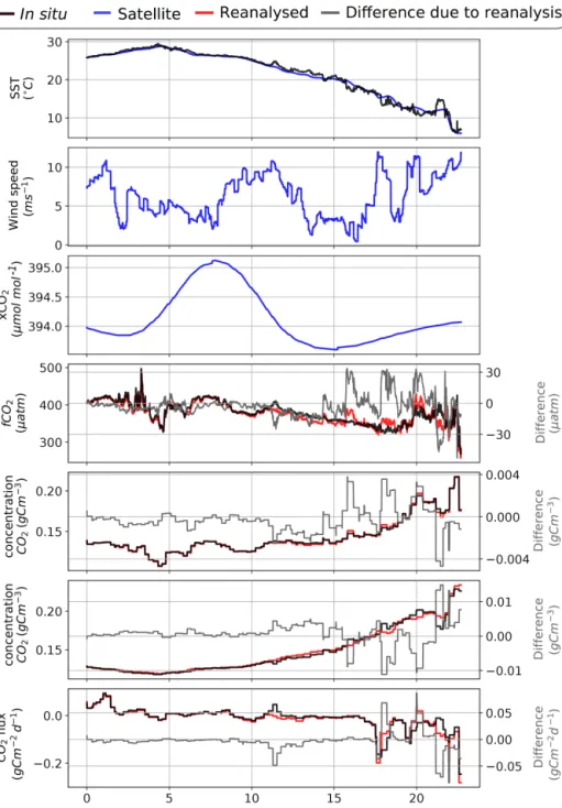
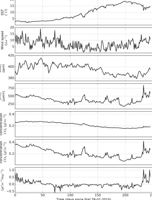
Theappend2insitu.pytool was then used to append Flux- Engine output to the original input data file for the Kitidis and Brown (2017) dataset. The output from this tool enables the user to visualise FluxEngine output (including any additional input data such as the Cross-Calibrated Multi-Platform (CCMP) wind speed data) as a time series alongside all other in situ data. Figure 4 shows the time series of SST,fCO₂, andxCO₂(from the downloaded cruise data). Plotted alongside these are the corresponding CCMP wind speed data and the calculated concentrations and fluxes using the original and reanalysedfCO₂data.

3.2 Case study 2: calculating CO₂fluxes from Östergarnsholm fixed station data

In this section the new capabilities for calculating gas fluxes from fixed stations is demonstrated using data from the long-term monitoring station at Östergarnsholm. The Öster- garnsholm station is situated in the Baltic Sea (57.42^◦N, 18.99^◦E) and is part of the Integrated Carbon Observation System (ICOS) infrastructure. The station was originally established in 1995 with the aim of collecting data on the marine atmospheric boundary layer to support research on the exchange of heat, momentum, and CO₂ between the atmosphere and ocean. It is equipped with instruments to measure (amongst other parameters) profiles of wind speed, water temperature, and aqueousfCO₂.

The new FluxEngine support for calculating gas fluxes from fixed stations uses the temporal dimension of the input files, creating output files of the same dimension that can

be easily visualised as a time series. Data for the Östergar- nsholm monitoring station covering a period from 28 January to 9 September 2015 were downloaded from the data repository (Rutgersson, 2017). These data contain in situ measurements forfCO2, salinity, and temperature; model reanalysis air pressure at sea level from the National Centers for Environmental Prediction and the National Center for At- mospheric Research (NCEP/NCAR) dataset (Kalnay et al., 1996);xCO₂from the NOAA ESRL GLOBALVIEW dataset (GLOBALVIEW-CO2, 2013); and World Ocean Atlas salinity data (Boyer et al., 2013). CCMP wind speed data were extracted and added to the tab-delimited in situ dataset using the same method as used in case study 1 (Sect. 3.1). For gridded input data, values were extracted from the single grid point containing the Östergarnsholm station location and were selected from a global 1^◦×1^◦projected grid.

Thetext2ncdf.pytool was configured to convert the text- formatted data file into a single netCDF file using a temporal resolution of 1 d. This produced a netCDF file with a temporal dimension size of 246 d, containing the daily mean value for each of the 246 d covered by the dataset. For this case study, FluxEngine was configured to use this file as input.

The flux calculation used the rapid model (Woolf et al., 2016) with the Nightingale et al. (2000) wind-based gas transfer velocity parameterisation and was performed using the original in situ fCO₂ and SST data. The temporal resolution was set to provide daily calculations for each of the 246 d, allowing seasonal variations to be observed.

FluxEngine supports arbitrary temporal resolutions to within minute precision and the choice predominantly depends on the resolution of the available data and the particular research questions to be addressed. FluxEngine was configured to write output into a single netCDF file as a time series. The

(9)

Figure 4.Time series of the (Kitidis and Brown, 2017) in situ campaign data with the sea-to-air CO₂flux as calculated by FluxEngine using the Ho et al. (2006) gas transfer velocity parameterisation. The results from the reanalysedfCO₂values are shown in red to distinguish them from the original data. The differences infCO₂, sub-skin, and interface CO₂concentration, and sea-to-air CO₂flux, resulting from the reanalysis, are shown in grey (reanalysed minus original).

in situfCO₂and SST measurements were assumed to represent the conditions at the bottom of the mass boundary layer and the concentrations at the top of the mass boundary layer were estimated by configuring the FluxEngine to estimate the skin temperature using the in situ SST – 0.17 (which is based on the work of Donlon et al., 2002).

Figure 5 shows the time series of SST, wind speed,xCO₂, fCO₂, concentration of CO₂, and calculated sea-to-air CO₂ flux. There is a moderate negative flux (ocean sink of CO₂) throughout most of the sampled period, which switched to a positive flux (outgassing to the atmosphere) during win- ter months. At approximately day 130, there is a local upwelling event which results in an incursion of CO₂-rich cold

(10)

Figure 5.FluxEngine output file using data from Östergarnsholm station over the 246 d period. Example components of the sea-to-air flux calculation are shown alongside the calculated CO₂flux.

water. This results in an increase infCO₂of approximately 250 µatm; however, coincident low wind speed means that there was little change in the flux during this event.

3.3 Case study 3: surfactant suppression of N₂O gas fluxes using the MEMENTO database

Nitrous oxide (N₂O) and methane (CH₄) are both climati- cally important gases. In the troposphere, they act as green- house gases (IPCC, 2013), whereas stratospheric N₂O is the major source for nitric oxide radicals, which are involved in one of the main ozone reaction cycles (Ravishankara et al., 2009). Source estimates indicate that the world’s oceans play a major role in the global budget of atmospheric N₂O and

a minor role in the case of CH₄(IPCC, 2013). Oligotrophic ocean areas are near equilibrium with the atmosphere and, consequently, make only a relatively small contribution to overall oceanic emissions, whereas biologically productive regions (e.g. estuaries, shelves, and coastal upwelling areas) appear to be responsible for the major fraction of the N2O and CH4emissions (Bakker et al., 2014).

Surfactants are surface-active compounds that can suppress turbulence at the sea surface thus altering air–sea gas exchange (McKenna and Bock, 2006; Pereira et al., 2016;

Salter et al., 2011). There is growing evidence from field and laboratory studies that naturally occurring surfactants can significantly reduce the flux of N₂O across the water–

(11)

atmosphere interface (Kock et al., 2012; Mesarchaki et al., 2015).

Previous work, which studied CO₂fluxes, found that surfactants potentially reduce the annual net integrated CO₂ flux by up to 9 % in the Atlantic Ocean (Pereira et al., 2018). Here, we use FluxEngine to apply the methodology of Pereira et al. (2018) to in situ data from the MEMENTO (MarinE MethanE and NiTrous Oxide) database (Kock and Bange, 2015) in order to estimate the equivalent suppression effect on the exchange of N₂O between ocean and atmosphere.

While FluxEngine is able to calculate sea-to-air fluxes of both N2O and CH4, we confined our analysis to N2O because of the sparsity of CH4 data. In situ and 1^◦×1^◦gridded monthly mean atmospheric and ocean partial pressure of N2O, sea surface temperature, and salinity were obtained from the MEMENTO database for the Atlantic Meridional Transect (AMT) cruise (AMT-24, JR303), which took place between September and November 2014 (Brown and Rees, 2018). These data were supplemented with Earth observation wind speed,U₁₀, from the CCMP dataset and modelled air pressure from the European Centre for Medium-Range Weather Forecasts (ECMWF). All input data were gridded to monthly means with a 1^◦×1^◦resolution.

A custom gas transfer velocity parameterisation was implemented following the template provided in the toolbox to calculate the gas transfer suppression due to biological surfactants in surface waters. This parameterisation uses the gas transfer velocity by Nightingale et al. (2000) com- bined with an estimate of the degree of surfactant suppression from Pereira et al. (2018). The method described by Pereira et al. (2018) used sea surface temperature to estimate surfactant suppression, meaning that no additional input data fields were needed. FluxEngine was configured to use the rapid flux model (Woolf et al., 2016) and run once with the standard Nightingale et al. (2000) gas transfer parameterisation (no suppression case) and then again using the Pereira et al. (2018) parameterisation (suppression case).

This new gas transfer parameterisation is now freely available within the FluxEngine (and can be selected by specify- ingk_Nightingale2000_with_surfactant_suppressionfor the k_parameterisationoption).

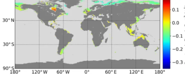
After calculating the air-to-sea N2O fluxes, we removed negative (atmosphere to ocean) fluxes. The fluxes for each grid cell (within which at least one in situ measurement ex- ists) are shown in Fig. 6a, while the difference in sea-to-air flux due to surfactant suppression is shown in Fig. 6b. The largest fluxes occur in the tropics and subtropical part of the AMT cruise track (Fig. 6a). Suppression of the gas transfer reduces the magnitude of the air–sea flux and the largest ab- solute suppression is also seen in the tropics and subtropical regions (Fig. 6a and b).

The append2insitu.pyutility was used to combine Flux- Engine output with the original in situ data. The time series are shown in Fig. 6c for SST, wind speed, atmospheric

and aqueous N2O, and sea-to-air N2O flux. The net fluxes along the transect are generally small and in both directions. The overall mean (and standard deviation) flux was 5.7×10⁻² (±5.7×10⁻²) g N₂O m⁻²d⁻¹ (no suppression) and 5.0×10⁻²(±4.8×10⁻²) g N₂O m⁻²d⁻¹(suppression), indicating in both cases a small net flux into the ocean. There was a mean flux suppression due to surfactants of 13 % for the entire dataset.

3.4 Case study 4: gas transfer velocity

parameterisation using turbulent kinetic energy dissipation rate

The gas transfer velocity,kin Eqs. (1) and (2), is determined by the turbulent mixing near the ocean surface (Jähne et al., 1987). While it is common to estimate gas transfer using a polynomial relationship with wind speed, turbulence in the upper ocean is influenced by additional physical processes that are independent, or not solely dependent, on the wind.

These include wave breaking, shear stress due to geostrophic currents, wind–wave–current interactions, bottom-generated turbulence, tidal forces, and precipitation (Villas Bôas et al., 2019; Zappa et al., 2007; Zhao et al., 2018).

In this case study we apply a gas transfer velocity parameterisation based on turbulent kinetic energy dissipation rate (ε), as developed by Zappa et al. (2007), to quantify the impact of wind- and wave-driven turbulence on sea-to-air CO₂. Zappa et al. (2007) used direct measurements ofkandεin aquatic and shallow marine regions to derive the following relationship:

k=0.419Sc^−0.5(εv)^0.25, (3)

where k is the gas transfer velocity (m s⁻¹), Sc is the Schmidt number, ε is the turbulent kinetic energy dissipation rate (W kg⁻¹), and v is the kinematic viscosity of water (m²s⁻¹). We calculate the monthly mean ε using the monthly mean wave (swell, secondary swell, and wind waves) to ocean turbulent kinetic energy flux (FOC) provided by the WAVEWATCH III model reanalysis (WAVE- WATCH III development group, 2016). The mean dissipation rate of turbulent kinetic energy,εmean, is calculated us- ingεmean=FOC/(ρz_max), whereρis the density of sea water (taken to be 1026 kg m⁻³), and z_max is the maximum depth over which dissipation is assumed to occur (taken as 10 m from Fig. 8 of Craig and Banner, 1994). This provides the mean total dissipation rate through the volume of water.

Equation (3) is valid forεmeasurements near the surface (of the order of 0.1 to 0.2 m), andεis known to decrease expo- nentially with depth. To estimateε at a depth of 0.2 m, we first fit an exponential function to the curve ofεfrom Fig. 8 of Craig and Banner (1994) which gave

ε=βexp(0.20z+0.78), (4)

wherezis depth andβ=1.86×10⁻³. Normalising this function to have a meanε equal toε_mean allowsε at any depth

(12)

Figure 6. (a)Sea-to-air N₂O flux taking into account surfactant suppression.(b)Change in N₂O flux resulting from surfactant suppression.

(c)Time series of SST, wind speed, atmospheric N₂O, aqueous N₂O, and sea-to-air flux.

to be determined. This was done by fitting β to minimise the difference betweenεmeancalculated from FOC andεmean

calculated from Eq. (4) to produce separate depth relation- ships withεfor each individual grid cell. Finally, the dissipation rate at 0.2 m was calculated by substituting z=0.2 into the final depth relationship. The process of fitting of the depth relationship and calculatingεat depthz=0.2 was implemented using a custom preprocessing function that is

included as an example in the FluxEngine download. This demonstrates how preprocessing functions can be used to perform complex data processing.

FluxEngine was then used to calculate monthly sea-to- air CO₂fluxes, globally, for 2010. All inputs to FluxEngine were provided as monthly averages with a 1^◦×1^◦ resolution. The additional input data were wind speed data from WAVEWATCH III reanalysis forcing field (WAVE-

(13)

WATCH III development group, 2016), sea surface temperature from Reynolds Optimum Interpolation Sea Sur- face Temperature dataset (OISST; Reynolds et al., 2007), salinity data from the NOAA World Ocean Atlas (Zweng et al., 2018), xCO₂ from the GLOBALVIEW-CO2 dataset (GLOBALVIEW-CO2, 2013), andfCO₂data from the SO- CAT derived sea-to-air CO₂flux reference dataset for 2010 (Woolf et al., 2019). Since the Zappa et al. (2007) relationship was parameterised in low to moderate wind speeds and in shallow marine environments, a mask was set in the configuration file to constrain the calculation to grid cells with wind speeds less than 10 m s⁻¹and shelf sea water depths between 20 and 200 m; then the analysis repeated with depths between 20 and 500 m. These depth ranges were chosen to be consistent with previous studies (e.g. Laruelle et al., 2018;

Shutler et al., 2016), and the General Bathymetric Chart of the Oceans (GEBCO) Digital Atlas bathymetry was used for this masking (GEBCO, 2003).

The ofluxghg_flux_budgets.py tool was used to compute the annual integrated net sea-to-air flux in all shelf sea regions. Collectively, the global shelf seas result in a net integrated flux into the ocean (sink) of 0.57 to 0.78 Pg C for 2010, where the range is due to the two shelf definitions. These results are within the bounds of those determined by previous studies (0.2–1 Pg C yr⁻¹ from Laruelle et al., 2017, 2018).

However we note that all previous studies have used wind speed for calculating gas exchange. Repeating the analysis with a wind-speed-based gas transfer velocity (Wanninkhof, 2014) instead of Eq. (4) gives an ∼8 % smaller net integrated flux of 0.53 to 0.72 Pg C. This result could suggest that published values of the global shelf sea CO2sink (calculated using wind speed gas transfer) are underestimated, as they do not fully account for wind–wave–current interactions and whitecapping. Figure 7 shows the resulting mean annual sea-to-air CO₂flux in 2010 for global shelf seas. FluxEngine has the capability to use non-wind-driven gas transfer parameterisations, allowing more physically based approaches to be evaluated such as the use of ε. The first synoptic-scale observation-based estimates ofεcould soon be possible from space using Doppler techniques (e.g. Ardhuin et al., 2019).

4 Future developments

The FluxEngine toolbox will continue to be developed in response to new advances in research and further user up- take will be encouraged through the provision of iPython Jupyter Notebook tutorials. There are currently four interactive Jupyter Notebook tutorials available within the Flux- Engine v3.0 download and these correspond to the first three case studies presented in this paper as well as an additional introductory tutorial. These interactive notebooks allow users to investigate the toolbox without the need to install any additional software. Users are able to modify and rerun the notebook and immediately see the impact of any changes.

Figure 7.Mean annual sea-to-air CO₂flux of shelf seas in 2010 using the Zappa et al. (2007) gas transfer relationship for all regions and months with wind speeds 0 to 10 m s⁻¹. Shelf regions are defined as having depths between 20 and 200 m.

This approach has been previously used by the authors for supporting collaborative research and summer school teaching. Additional Jupyter Notebook tutorials could be written to provide worked examples of (i) driving FluxEngine with a custom Python script to perform a sensitivity or ensemble analysis, (ii) using the FluxEngine to study a freshwater envi- ronment, or (iii) using the verification tools module to verify custom changes and extensions to the toolbox. All notebooks will be maintained so that they remain available and relevant to future versions of the FluxEngine.

5 Conclusions

FluxEngine is an open-source and freely available software toolbox that provides standardised and verified calculations of gas exchange and net integrated fluxes between the ocean and atmosphere, and the toolbox is now being used by in situ, Earth observation, and modelling scientific communities. The development of the toolbox was driven by the desire to reduce duplication of effort, to facilitate collaboration between different research communities, and to accelerate advancements in air–sea gas flux research and monitoring.

Building on Shutler et al. (2016), who demonstrated the toolbox and verified the accuracy of the calculations, this paper demonstrates new capabilities that considerably broadens the scope of research questions that can be addressed using FluxEngine. Version 3.0 can now be easily installed and ex- ecuted on a desktop or laptop computer and does not require specialist hardware or software libraries. It can be used as a Python library or as a set of stand-alone command-line utilities. The toolbox now includes an extensive suite of tools for calculating gas fluxes directly from in situ data. Collec- tively, these improvements have streamlined the process for extending the toolbox and will allow users to easily take ad- vantage of newly developed gas transfer velocity parameterisations and/or new sources of input data. These new tools and the toolbox are fully compatible with the internationally established data structures being used by the SOCAT and the MEMENTO communities.

(14)

The inclusion of the handling of CH4 and N2O sea–air gas fluxes is intended to directly support those communities studying these gases. Significant international research focus and effort is now being directed to collating data on these gases towards monitoring and understanding their spatial distribution and variability.

The FluxEngine toolbox will continue to be updated as new approaches become available. Further development will be guided by the needs of the international research and monitoring communities, so we welcome feedback from users on all aspects of the toolbox.

Code availability. FluxEngine is an open-source software and is available with a creative commons license via https://github.com/

oceanflux-ghg/FluxEngine (last access: 6 December 2019, GitHub, 2019a). FluxEngine is in constant development and historic versions are available via GitHub. To access the specific version used to conduct the case studies in Sect. 3, please access the v3.0 release via https://github.com/oceanflux-ghg/FluxEngine/releases/tag/v3.0 (last access: 6 December 2019, GitHub, 2019b).

(15)

Appendix A: Utility names and descriptions

Several additional utilities are provided as Python scripts to support the installation, verification, execution, and processing of output, and these are listed in Table A1.

Table A1.Description of the bundled tools and scripts that are included in FluxEngine. Each tool can be used as a stand-alone command-line tool or used as a Python package.

Utility Description

append2insitu.py Appends netCDF data (e.g. FluxEngine output) to text-

formatted data files as new columns. Matching rows by longi- tude, latitude, and time.

install_dependencies_macos.py, install_dependencies_ubuntu.py

Installation scripts. Installation instructions are provided for Windows users inFluxEngineV3_instructions.pdf.

ncdf2text.py Converts netCDF output files to text-formatted files.

ofluxghg_flux_budgets.py Calculates total monthly and annual gas flux from FluxEngine output. Supports global and regional analysis.

ofluxghg_run.py Commandline tool used to run FluxEngine.

reanalyse_socat_driver.py Uses satellite sea surface temperature to reanalyse CO₂fugacity and partial pressure data to a consistent temperature and depth (see Goddijn-Murphy et al., 2015)

run_full_verification.py Runs an extended verification procedure. Required additional data from (Holding et al., 2018).

text2ncdf.py Converts text-formatted data files into FluxEngine compatible netCDF format.

validation_tools.py, compare_net_budgets.py Contains Python functions to aid verification of FluxEngine output to a reference dataset.

verify_socatv4_sst_salinity_ gradients_N00.py, verify_takahashi09.py

Verifies that FluxEngine has been installed correctly by compar- ing output with a reference data from SOCAT-derived or Taka- hashi climatologies, respectively.

(16)

Appendix B: Datasets used

Table B1 provides details of each of the datasets that were used in the case studies.

Table B1.The Earth observation in situ, model, and climatology data used in this research.

Name Parameter(s) Reference and source

CCMP v2 (Cross-Calibrated Multi-Platform) U₁₀(wind speed at 10 m) Atlas et al. (2011)

http://www.remss.com/measurements/ccmp/

(last access: 6 December 2019) OISST (Optimum Interpolation Sea Surface

Temperature)

Sea surface temperature (SST)

Reynolds et al. (2007)

https://www.ncdc.noaa.gov/oisst (last access: 6 Decem- ber 2019)

GLOBALVIEW-CO2 xCO₂(molar fraction of

CO₂in dry air)

GLOBALVIEW-CO2 (2013)

https://www.esrl.noaa.gov/gmd/ccgg/globalview/co2/

co2_intro.html (last access: 6 December 2019) National Centers for Environmental Predic-

tion, National Center for Atmospheric Research (NCEP/NCAR)

Air pressure Kalnay et al. (1996)

https://www.esrl.noaa.gov/psd/data/gridded/data.ncep.

reanalysis.pressure.html (last access: 6 December 2019) Underway data from the James Clark cruise

(74JC20131009)

SST, salinity, air pressure, fCO₂

Kitidis and Brown (2017)

https://doi.pangaea.de/10.1594/PANGAEA.878492 Underway data from the Benguela Stream

cruise (642B20131005)

Schuster (2016)

https://doi.org/10.1594/PANGAEA.852980 Underway data from the Atlantic Companion

cruise (77CN20131004)

Steinhoff et al. (2016)

https://doi.org/10.1594/PANGAEA.852786 Underway data from the REYKJAFOSS cruise

(64RJ20131017)

SST, salinity, air pressure, fCO₂,xCO₂

Wanninkhof and Pierrot (2016)

https://doi.org/10.1594/PANGAEA.866092 Östergarnsholm station (77FS20150128) Air pressure, salinity, SST,

xCO₂(air),fCO₂(water)

Rutgersson (2017)

https://doi.pangaea.de/10.1594/PANGAEA.878531 MarinE MethanE and NiTrous Oxide database

(MEMENTO)

SST,pN₂O_air,pN₂Owater Kock and Bange (2015) https://memento.geomar.de/

(last access: 6 December 2019) National Oceanic and Atmospheric Administra-

tion, US (NOAA) WAVEWATCH III

U₁₀ (wind speed at 10 m), FOC (wave to turbulent kinetic energy)

WAVEWATCH III development group (2016)

Interpolated and reanalysedfCO₂ field originating from the SOCAT dataset

fCO₂(interpolated) Dataset methodology: Woolf et al. (2019) ResultantfCO₂data: Holding et al. (2018) https://doi.pangaea.de/10.1594/PANGAEA.890118 Original SOCAT dataset: Bakker et al. (2016)

https://www.socat.info/ (last access: 6 December 2019)

(17)

Appendix C: Summary of main toolbox features

Table C1 lists the main features of the FluxEngine toolbox with summaries of their impact for the accurate calculation of atmosphere–ocean gas fluxes.

Table C1.An overview of the key features provided by the FluxEngine software toolkit and their relevance or use for atmosphere–ocean gas exchange.

Feature or option Description Example impact or use

Ability to choose the structure of the bulk gas flux calculation or formulation

The user can choose their bulk formulation but a formulation based on concentration differences (i.e. containing two solubilities) is advised. This advised formulation enables near- surface temperature and salinity gradients to be included. For reasoning and examples of this advice, please see Woolf et al. (2016, 2019) and Sect. 1b of Shutler et al. (2016).

Woolf et al. (2019) shows that ignoring vertical temperature and salinity gradients for 2010 results in a 0.35 Pg C (12 %) bias or underestimate in the oceanic sink of CO₂.

User-selectable gas transfer velocity parameterisations

The toolbox includes 14 published wind speed parameterisations and one mean square slope parameterisation, along with a generic user- configurable wind speed parameterisation (see Sect. 7 of the FluxEngine manual). Custom user parameterisations can be added using a Python template (Sect. 9.2 of the FluxEngine manual).

Wrobel and Piskozub (2016) showed that the (model) uncertainty due to the choice of quadratic gas transfer parameterisation led to a 9 % difference in the gas transfer velocity for the North Atlantic and subpolar waters. This uncertainty increased to 65 % when all parameterisations were consid- ered.

ReanalysefCO₂data to a reference temperature and depth

The user can reanalyse paired in situfCO₂and SST measurements to a consistent depth using a reference temperature dataset as described by Goddijn-Murphy et al. (2015).

This removes unknown biases due to paired data originating from multiple depths. The depth of in situ data can vary during a single research cruise (e.g. due to sea state or ballasting) and measurements from varying depths become a more significant problem when using large collated datasets collected using different measurement systems.

User-selectable gas input data types

The user can input atmospheric and marine gas data as partial pressures, fugacities, or concentrations.

This allows for a wider range of poorly soluble gases to be analysed.

Flexibility to calculate air–sea gas fluxes of multiple poorly soluble gases

The toolbox supports user-definable sea-to-air gas flux calculations for CO₂, CH₄, and N₂O.

This paper estimates that surfactants can suppress N₂O gas fluxes by up to 13 % in the North Atlantic.

Accounting for the impact of rain on air–sea gas fluxes

Users can investigate methods that include the different influences that rain can have on air–

sea gas fluxes.

Ashton et al. (2016) estimated that rain-driven gas transfer and wet deposition of carbon increases the annual oceanic integrated net sink of CO2by up to 6 %.

Flexible input data specification and support for in situ data

Tools are provided to support user-specified grid size, temporal resolution, naming conventions and directory structure, automatic unit conversion, and conversion between text- (ASCII) and netCDF-formatted data files.

Allows for a wide range of data to be easily used and analysed by the user and the FluxEngine outputs can be easily incorporated into the users original in situ dataset.

Calculate integrated net gas fluxes

A tool for calculating global or regional integrated net gas fluxes (e.g. CO2 sink) from netCDF air–sea gas flux data is provided. This enables user-defined land, ice, and region of interest masks to be used and there are multiple options for handling the impact of sea ice.

Shutler et al. (2016) showed that the calculated net CO₂ fluxes can vary by 14 % for the European shelf sea simply due to differing shelf sea masks, highlighting the need for traceable methods and masks for net flux calculations.

Input data uncertainty analysis Users can add random noise (with user-defined variance and bias) to any input dataset. This enables the users to investigate the impact of input data uncertainties on their air–sea gas flux calculation (e.g. through using an ensemble approach).

Ashton et al. (2016) identified that known uncertainties due to random fluctuations in the input data resulted in a±1 % variation in the monthly net integrated CO₂sink.

Land et al. (2013) identified that the dominant source of uncertainty in Arctic air–sea gas flux calculations was due to bias in wind speed data (and its impact on the wind-speed- based gas transfer velocity).

(18)

Appendix D: Installation, verification, and benchmarking

Installation tools or instructions are provided in the FluxEngine root directory for the following operating systems: Ubuntu/Debian-based Linux (in- stall_dependendies_ubuntu.sh), Apple Mac (in- stall_dependencies_macos.sh), and Windows (instructions are within FluxEngineV3_instructions.pdf).

Two verification utilities (also located in the root directory) are provided (verify_takahashi09.py andverify_socatv4_sst_salinity_gradients_N00.py). These can be used to verify the successful installation of Flux- Engine by running standard global sea-to-air CO2gas flux calculations and net integrated fluxes using the (Takahashi et al., 2009) sea-to-air CO2 flux climatology (for the year 2000) and the Woolf et al. (2019) Surface Ocean CO₂ ATlas (SOCAT; Bakker et al., 2016) sea-to-air CO₂ flux reference dataset for the year 2010. Both of these datasets are contained within Holding et al. (2018) and the verification process compares the output from a test run of the toolbox with the reference data published in Holding et al. (2018).

The installation is deemed successful if all results are identi- cal to the reference dataset within a precision of five decimal places. An additional utility (run_full_verification.py) enables the user to perform a more detailed verification of different user-defined options that exploit the Woolf et al. (2019) reference dataset. This executes a suite of 12 different configurations and scenarios, the justification for which is described within Woolf et al. (2019). Owing to the large volume of data required to execute and verify all of these scenarios, the verification data are not packaged with the standard FluxEngine download but are all freely available and contained within Holding et al. (2018).

To provide an indication of the execution time, a benchmarking analysis was performed using an Intel Core i5 2.7 GHz laptop processor with 8GB RAM running MacOS El Capitan. The automatic installation took∼3 min to complete and the basic verification script using the Woolf et al. (2019) reference dataset (involving a global 1 year analysis of the gas fluxes for 2010, monthly temporal resolution, and 1^◦×1^◦spatial resolution) took approximately 6 min to complete. As the flux calculation is sequential for each grid cell, the execution time scales approximately linearly with the number of grid points and number of time steps. Hence, doubling the temporal resolution will approximately double the execution time, whilst doubling the resolution of both spatial dimensions will lead to a factor of 4 increase in execution time.