Air–sea fluxes of greenhouse gases and oxygen in the northern Benguela Current region during upwelling events

(1)

https://doi.org/10.5194/bg-16-4065-2019

Air–sea fluxes of greenhouse gases and oxygen in the northern Benguela Current region during upwelling events

Eric J. Morgan^1,a, Jost V. Lavric¹, Damian L. Arévalo-Martínez², Hermann W. Bange², Tobias Steinhoff², Thomas Seifert¹, and Martin Heimann^1,3

1Biogeochemical Systems Department, Max Planck Institute for Biogeochemistry, Jena, Germany

2GEOMAR Helmholtz Centre for Ocean Research, Kiel, Germany

3Institute for Atmospheric and Earth System Research (INAR)/Physics, University of Helsinki, Helsinki, Finland

anow at: Scripps Institution of Oceanography, University of California, San Diego, La Jolla, CA, USA Correspondence:Eric J. Morgan (ejmorgan@ucsd.edu)

Received: 20 March 2019 – Discussion started: 26 March 2019

Revised: 13 September 2019 – Accepted: 18 September 2019 – Published: 21 October 2019

Abstract. Ground-based atmospheric observations of CO₂, δ(O₂/N₂), N₂O, and CH₄ were used to make estimates of the air–sea fluxes of these species from the Lüderitz and Walvis Bay upwelling cells in the northern Benguela region, during upwelling events. Average flux densities (±1σ) were 0.65±0.4 µmol m⁻²s⁻¹for CO2,−5.1±2.5 µmol m⁻²s⁻¹ for O2 (as APO), 0.61±0.5 nmol m⁻²s⁻¹ for N2O, and 4.8±6.3 nmol m⁻²s⁻¹for CH4. A comparison of our top- down (i.e., inferred from atmospheric anomalies) flux estimates with shipboard-based measurements showed that the two approaches agreed within ±55 % on average, though the degree of agreement varied by species and was best for CO₂. Since the top-down method overestimated the flux density relative to the shipboard-based approach for all species, we also present flux density estimates that have been tuned to best match the shipboard fluxes. During the study, upwelling events were sources of CO₂, N₂O, and CH₄ to the atmosphere. N₂O fluxes were fairly low, in accordance with previous work suggesting that the evasion of this gas from the Benguela is smaller than for other eastern boundary upwelling systems (EBUS). Conversely, CH4release was quite high for the marine environment, a result that supports studies that indicated a large sedimentary source of CH4in the Walvis Bay area. These results demonstrate the suitability of atmospheric time series for characterizing the temporal variability of upwelling events and their influence on the overall marine greenhouse gas (GHG) emissions from the northern Benguela region.

1 Introduction

Coastal margins, particularly those associated with the upwelling of nutrient-rich subsurface waters, are biogeochemi- cally active regions (Levin et al., 2015). The air–sea fluxes of greenhouse gases (GHGs, referring to the long-lived greenhouse gases CO₂, N₂O, and CH₄) from or to such systems can vary markedly, both spatially and temporally (Torres et al., 1999; Naqvi et al., 2010; Evans et al., 2011; Reimer et al., 2013; Capone and Hutchins, 2013). This is because both the occurrence and intensity of coastal upwelling events are variable in nature, as they are forced by surface winds that occur under specific synoptic conditions; even large events happen only on a timescale of days (Blanke et al., 2005;

Goubanova et al., 2013; Desbiolles et al., 2014a, b). The sporadic nature of upwelling implies that observations made during short-term campaigns may not capture the full range of flux variability.

Upwelled water is usually colder than the surrounding surface water, which means that the solubility of dissolved gases will decrease with increasing temperature as water masses warm at the surface. A competing influence for CO₂ ex- ists in that the supply of inorganic nutrients from an upwelling event can lead to blooms of phytoplankton and a net drawdown of atmospheric CO₂. For O₂, the ventilation of deeper water masses can drive a net flux into the ocean, or net productivity can create oversaturation of dissolved O₂. Hence, coastal upwelling regions can oscillate between being sources and sinks of O₂ and CO₂ (Torres et al., 1999;

Santana-Casiano et al., 2009; González-Dávila et al., 2009;

(2)

Gregor and Monteiro, 2013; Cao et al., 2014; Evans et al., 2015). Most coastal upwelling systems are also known to be regional hotspots of N₂O emissions (Bange et al., 2001;

Lueker et al., 2003; Cornejo et al., 2006; Bianchi et al., 2012;

Arévalo-Martínez et al., 2015; Babbin et al., 2015). Air–sea fluxes of CH₄are less constrained, but may be a significant term in the marine CH₄budget (Rehder et al., 2002; Sansone et al., 2001).

A well-established method of estimating budgets of air–

sea fluxes for GHGs in upwelling regions is to take wind fields and interpolated or representative surface measurements, use them to calculate a flux density, and scale it up over a selected area. The high variability of air–sea exchange means that determining budgets of air–sea fluxes of GHGs is challenging without a high degree of spatial and temporal sampling. We refer to this in the text as the “bottom-up”

approach.

Another approach, and one that sidesteps some of these difficulties, is to use a “top-down method”, i.e., using atmospheric measurements to infer fluxes from the surface, using simple models (Lueker et al., 2003; Lueker, 2004; Nevi- son et al., 2004; Thompson et al., 2007; Yamagishi et al., 2008) or more complex inverse methods (e.g., Rödenbeck et al., 2008). A simple top-down approach has been suc- cessfully employed to detect air–sea fluxes of CO₂, O₂, and N₂O from the California Current region from a coastal atmospheric monitoring station at Trinidad Head, California (Lueker et al., 2003; Lueker, 2004; Nevison et al., 2004).

This work motivated our own efforts to see whether anomalies related to upwelling events could be seen in continuous observations from an atmospheric measurement site located near the upwelling region in the northern Benguela region, which is one of the least sampled EBUS for air–sea fluxes of GHGs (Nevison et al., 2004; Naqvi et al., 2010; Laruelle et al., 2014).

In this study, 2 years of continuous observations from a ground-based atmospheric observatory for greenhouse gases, the Namib Desert Atmospheric Observatory (NDAO), were utilized to create top-down estimates of the air–sea flux densities of CO₂, O₂, N₂O, and CH₄ from the Lüderitz and Walvis Bay upwelling cells, during upwelling events. We fo- cus on individual upwelling events as we expect them to be distinguishable from other sources of intraseasonal variability based on their apparent stoichiometry in the atmosphere and because there are relatively few observation-based studies from this region, relative to other EBUS. This area of the coastal shelf, stretching from ca. 22 to 28^◦S, is subject to the strongest surface winds and upwelling fluxes of water in the region, and surface chlorophyll is at a minimum (Lut- jeharms and Meeuwis, 1987; Hagen et al., 2001; Demarcq et al., 2007; Veitch et al., 2009; Hutchings et al., 2009). These estimates were then compared with shipboard measurements from a cruise in the two upwelling centers.

2 Methods

2.1 Atmospheric measurements at the Namib Desert Atmospheric Observatory

Continuous measurements of CO₂, atmospheric oxygen, N₂O, CH₄, and CO were made at the Namib Desert Atmo- spheric Observatory (NDAO), a background site located at 23.563^◦S, 15.045^◦E, in the central Namib Desert, at Goba- beb Research and Training Centre. This dataset is provided as a Supplement to this paper, available online at: https:

//doi.org/10.5194/bg-16-1-2019-supplement. A full description of the measurement system is given in Morgan et al.

(2015). In brief, observations were made at a height of 21 m above ground level with a Picarro ESP-1000 cavity ring- down spectrometer (CRDS) for CO2and CH4, a Los Gatos N2O/CO-23d cavity-enhanced absorption spectrometer for N2O and CO, and an Oxzilla FC-II dual absolute and differ- ential oxygen analyzer forδ(O2/N2).

While the Picarro and Los Gatos analyzers measure continuously (data are recorded at approximately 0.5 and 1 Hz, respectively), the Oxzilla analyzer measures the difference between sample air and a reference tank, at a data rate of 0.01 Hz. Calibration of the instruments was done through four working secondary standards and instrument perfor- mance was periodically checked with “target” cylinders (i.e., tanks of known mole fraction which are regularly re- measured). Reference gases comprised dry ambient air and were stored in 50 L aluminum cylinders. Calibrations were run every 123 h for the Picarro and Los Gatos analyzers and every 71 h for the Oxzilla analyzer. All measurements were tied to primary standards on the following scales:

WMO X2007 for CO2, NOAA 2004 for CH4, NOAA 2006a for N2O, WMO X2004 for CO, and the Scripps Institution of Oceanography Scale forδ(O₂/N₂), as defined on 1 Au- gust 2012.

The average uncertainty for each species during the study period was 0.028 ppm for CO₂, 6.5 per meg for δ(O₂/N₂), 0.21 ppb for N₂O, 0.17 ppb for CH₄, and 0.15 ppb for CO. CO₂, N₂O, CH₄, and CO are all expressed as dry air mole fractions, in ppb or ppm (1 ppm=1 µmol mol⁻¹; 1 ppb=1 nmol mol⁻¹).

By convention, changes in atmospheric oxygen were quantified as the O₂/N₂ratio relative to a standard, in per meg units (Keeling and Shertz, 1992):

δ(O2/N2)=

(O₂/N₂)_sample (O₂/N₂)ref

−1

×10⁶. (1) In order to isolate the influence of air–sea exchanges on O₂/N₂, we have employed the use of a data-derived tracer, known as atmospheric potential oxygen (APO), which masks variations of O₂/N₂that are due to terrestrial biosphere exchange (Stephens et al., 1998). Variations in APO are thus primarily due to fossil fuel burning and air–sea gas exchange

(3)

of O2. APO is defined as APO=δ (O2/N2)+ 1.1

X_O₂(CO2−350) . (2)

Here 1.1 is the nominal global average oxidative ratio (OR;

1O₂/1CO₂on a mol/mol basis) for terrestrial photosynthe- sis and respiration (Severinghaus, 1995), andX_O₂is the mole fraction of oxygen in the atmosphere, 0.2095, as defined by the Scripps O₂Program scale; 350 is a reference CO₂value, and CO₂ is the in situ concentration of carbon dioxide, in ppm. APO andδ(O₂/N₂)are both expressed in per meg. In some instances it is useful to express APO in molar units that are of the same relative magnitude as the dry air mole fraction in ppm. This conversion is done by multiplyingδ(O₂/N₂)or APO byXO₂. We refer to this unit as parts per million equivalents, or “ppm eq”.

2.2 Remote sensing data

Following the reasoning of Goubanova et al. (2013), sea surface temperature (SST) data were obtained from the Re- mote Sensing Systems (http://www.remss.com/, last access:

28 December 2014) data archive. The Tropical Rainfall Mea- suring Mission (TRMM) Microwave Imager (TMI) daily op- timally interpolated SST product was selected. The major advantage of this instrument is its ability to measure SST through clouds, which are considerable over the coast, as the TMI measures frequencies in the microwave region (4–

11 GHz). The drawback of this dataset is that there are no data within 100 km of the coast. Large upwelling features, however, extend much farther out than this and are read- ily seen by the TMI (Goubanova et al., 2013). Even with this loss of near-shore data, the data coverage is still supe- rior to that of optical sensors like the Moderate-Resolution Imaging Spectroradiometer (MODIS). The TRMM SST data presented in this work are deseasonalized by subtracting a second harmonic fit to the data, as it showed a strong sea- sonal cycle which masked some of the intraseasonal variability when plotted as a time series.

Wind speed data for the South Atlantic were also derived from the TMI instrument on the TRMM satellite. This dataset is a level 3 product which gives the 10 m wind speed over marine areas within the sensor’s field of view. The 18.7 GHz channel data product was selected. Like the SST data, a major drawback of this dataset is the absence of data within 100 km of land.

Two surface chlorophyll products were used, both level 3 binned products that combined data from multiple satel- lites, accessed through the ESA GlobColour website (http:

//www.globcolour.info/, last access: 15 December 2014). The first is denoted CHL1-GSM; this dataset is a merged product of two different sensors (during the time period considered), MODIS and the Visible Infrared Imaging Radiome- ter Suite (VIIRS). The data are merged using the Garver–

Siegel–Maritorena (GSM) model, which blends the normal-

ized water-leaving radiances instead of Chlaconcentrations (Maritorena and Siegel, 2005). The second product is denoted CHL1-AVW; these data are merged using a weighted average method (AVW). Like CHL1-GSM, it combines data from MODIS and VIIRS for the time frame considered.

2.3 Atmospheric back-trajectories

Back-trajectories, which trace the path of a particle from a receptor point backwards in time, provide a history of recent atmospheric transport. Back-trajectories were simulated with the HYbrid Single Particle Lagrangian Integrated Trajectory (HYSPLIT) 4 model (Draxler and Hess, 1997, 1998) from NDAO for 120 h, for the entire time series. A new trajectory was calculated every 6 h, starting at 00:00 UTC, i.e., at 01:00, 07:00, 13:00, and 19:00 local time. The model was run with a spatial resolution of 1^◦×1^◦and a temporal resolution of 1 h.

A vertical cut-off of 10 km a.g.l. was used. Meteorological fields were obtained from the National Center for Environ- mental Prediction (NCEP) Global Data Assimilation System (GDAS).

2.4 Identification of upwelling events and selection of atmospheric anomalies

A subset of the coastal region was selected to represent the Lüderitz and Walvis Bay upwelling cells. The boundaries of this domain were at 13 and 15^◦E, 23 and 27^◦S (Fig. 1a), representing an ocean area of 56 196 km². This domain covers the continental shelf and a small portion of the continental slope; the mean water depth is 390 m. We selected this domain because it represented an area of the coast where strong upwelling occurs regularly (Demarcq et al., 2007), where this upwelling was spatially distinct from other upwelling cells reported in the literature (Lutjeharms and Meeuwis, 1987;

Veitch et al., 2009), and where upwelling was downwind of the station during upwelling events. These criteria were considered desirable because they would provide the best op- portunities for relating atmospheric anomalies to upwelling events. These determinations were based on analysis of our SST dataset and HYSPLIT back-trajectories.

Upwelling events were identified based on SST anomalies and 10 m wind speed anomalies. An event was determined to occur if the average deseasonalized SST of the domain was 0.5^◦C or lower than a smoothed, second-degree polynomial fit to the entire time series and the average 10 m wind speed of the study area was 2.5 m s⁻¹above a smoothed, second- degree polynomial fit to the wind data. These thresholds were determined through visual inspection of maps and time series of SST and wind speed data and are specific to the domain chosen, since the data considered were averages of the entire area. One standard deviation of the SST anomaly was 0.92^◦C, and 1 standard deviation of the wind speed anomaly was 3.1 m s⁻¹. Since the resolution of the SST and wind speed time series was daily, all higher-resolution data falling

(4)

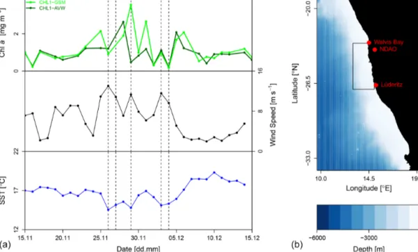
Figure 1.An example of an upwelling event at the end of 2013. The median chlorophyllaof the domain is shown over a period of 1 month, along with the domain-averaged 10 m wind speed and sea surface temperature(a). Days flagged as upwelling events are shown as dashed vertical lines. The Lüderitz–Walvis Bay domain is shown, overlain on a bathymetric map(b). Data are from Amante and Eakins (2009).

within a day during which an upwelling event occurred were similarly flagged.

Atmospheric anomalies associated with upwelling events were quantified against a baseline determined through a second-harmonic fit that was applied iteratively to all data, excluding all points that lay outside 1 standard deviation from the curve for the subsequent iteration. Small adjust- ments were made to the anomaly to raise or lower the curve in cases where it did not intersect with background values within ±5 d of the event. The NDAO data were filtered by wind (wind speeds greater than 2 m s⁻¹and wind direction within the NNW–SSW sector), as well as by back-trajectory to exclude anomalies which were not associated with marine air masses. For the latter, trajectories could not reside for more than 36 h of the total 120 h over land and could not travel more than 50 km inland past NDAO. A final data selection step was to exclude days that had CO values greater than 15 ppb above the baseline, to remove any time periods that may have been influenced by biomass burning. The filtered time series, with terrestrial influences removed, is shown in Fig. 2.

2.5 Top-down air–sea flux estimates

In order to estimate the surface flux associated with atmospheric anomalies due to upwelling events, the approach of Lueker et al. (2003) was adopted. A simple model was employed to describe the change in the concentration of a species within a well-mixed column of air as it moves over a

source region (Jacob, 1999):

1C=







F hq

1−e⁻^qx^U

, for 0≤x≤L, 1C_L

e⁻^q(x−L)^U

, forx≥L.

(3) Here1C is the concentration of the species of interest, in mol m⁻³, expressed as an anomaly against the background.

1Cis a function ofx, which is the distance to the observation point from the flux region.Lis the point at which the column (with height h, in meters) leaves this region, characterized by a constant flux,F, in mol m⁻²h⁻¹, and a constant wind speed,U, in m h⁻¹. After the column leaves the flux region (x≥L, i.e., when the coast is reached), the loss of1Cfrom its peak atL(1C_L) is governed by dilution due to mixing of background air. This requires the dilution rate constant,q, in h⁻¹, to be known.

We solved the equation forF by taking the other variables as follows:1Cwas determined from our atmospheric record (see Sect. 2.4), wind speeds (U) were obtained from satellite data (Sect. 2.2), and h was taken as the average height of the planetary boundary layer (PBL) for the Lüderitz–Walvis Bay domain over the course of any given event. PBL data were acquired from the European Centre for Medium-Range Weather Forecasting’s (ECMWF) ERA-Interim dataset (Dee et al., 1979).xwas taken as the length traveled along a back- trajectory from NDAO to the area affected by upwelling.

The dilution rate constant,q, was estimated by comparing measurements of CO₂and CH₄made during the RVMeteor cruise M99 (see Sect. 2.7). Back-trajectories from NDAO

(5)

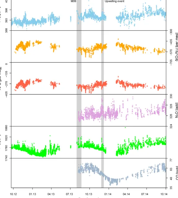
Figure 2.NDAO filtered time series. The NDAO time series, filtered based on back-trajectory and CO. The main measurands of the station are each plotted as 30 min averages. The duration of M99 and the upwelling event discussed in the main text are both demarcated with gray rectangles and denoted with a label. The presence of an upper bound in the CO data is due to its use as a filtering criterion.

were matched to the closest ship location at the appropriate time. Any back-trajectory points that were within 100 km of the ship – both horizontally and vertically – within the space of 1 h were identified, and a dilution rate constant was calculated for both CO₂and CH₄, as (Price et al., 2004)

q=1 t ln

CM99−Cb

CNDAO−Cb

, (4)

where C_M99 andC_NDAO are the mole fractions of CO₂ or CH₄, as measured in situ on theMeteoror at NDAO, andC_b is taken from the fit to the baseline of the NDAO time series for either species, as described in Sect. 2.4.tis the travel time along the back-trajectory, in hours. While this assumes that

there is no flux of the gas between the vessel and the station, we excluded instances when the anomaly was heavily influenced by surface fluxes by filtering for poor agreement between CO₂and CH₄. Fluxes of these gases are not well correlated and can go in opposite directions for summertime air–

sea fluxes, so we assume that it is unlikely that both values ofqwould be biased by the same amount. From 32 values of q we excluded all but 13 for poor agreement (excluding determinations with|q_CO₂−q_CH₄|>0.01). The average (±1σ) was taken to arrive at a single value, 0.011±0.006 h⁻¹. Since this is still a rough approximation, we also present estimates of the estimated flux, F, with a value of q tuned to pro-

(6)

vide the best agreement with an in situ flux estimate (see Sect. 2.8).

2.6 Estimated top-down flux density uncertainty Uncertainties were propagated in quadrature, e.g., σx=

q

σ_a²+σ_b², (5)

for operations involving addition or subtraction (x=a+b), and

σ_x= r

σa

a 2

+σ_b b

2

·x (6)

for operations involving multiplication or division (x=ab), whereσ is the uncertainty for a given variable. The uncertainty in1Cfor each species was the propagated analytical uncertainty (see Sect. 2.1) of the difference between the average ofCduring the maximum of the anomaly and the baseline, plus a small uncertainty term for the value of the baseline itself based on the standard deviation of 1000 simula- tions in which one-third of data were discarded and the curve fit repeated.x andLwere both taken as the standard deviation of the term calculated independently for eight HYSPLIT back-trajectories from NDAO within 0–50 h back from the anomaly detection. The uncertainty forUwas 1 standard deviation of wind speeds for the study domain within the 50 h period.

2.7 In situ measurements during RVMeteorcruise M99

Cruise M99 of the RV Meteor left Walvis Bay on 31 July 2013 and returned to port on 23 August. Continu- ous or semi-continuous measurements of atmospheric CO₂, N₂O, and CH₄, as well as dissolved CO₂, O₂, and N₂O, were conducted throughout the cruise. Flask samples were taken for discrete measurements ofδ(O₂/N₂).

Atmospheric measurements of CO₂and CH₄ were made with a CRDS analyzer (model G1301, Picarro Inc, Santa Clara, CA, USA) located in the atmospheric chemistry lab- oratory. The instrument’s internal pump was used to draw air through a 7 m length of 1/4⁰⁰SERTOflex tubing, at a flow rate of 150 mL min⁻¹. Inlets identical to those used at NDAO (Morgan et al., 2015) were placed on the starboard railing of the sixth superstructure deck, just above the atmospheric chemistry lab, at a total height of∼21 m above sea level. A second-order, instrument-specific water correction was per- formed in lieu of physical or chemical drying, identical to the method described in Morgan et al. (2015). As the instrument’s pressure control seemed to be affected by strong vessel motion, measurements were excluded if the cavity pressure deviated by more than 0.04 torr from the set point of 140 torr. Calibrations were conducted on average every 3 d and target measurements were made once per day. Reference

gases were calibrated at MPI-BGC GASLAB. The uncertainty, derived from the target measurements as at NDAO, was determined to be±0.03 ppm for CO₂and±0.43 ppb for CH₄. The dataset was filtered for contamination by the ship’s exhaust using the relative wind direction data from the ship’s meteorological instrumentation.

Flasks for δ(O₂/N₂) were taken in triplicate and con- nected in series downstream of a pump. The pump body and valve plates were aluminum, and the structured di- aphragms were made of PTFE. When in use the flow rate (3.2 L min⁻¹) was higher than the in situ analyzer flow rates (100–200 mL min⁻¹). Air was dried with magnesium per- chlorate. During sampling, the line was flushed for 5 min before any air was directed to the flasks, and then a bypass valve was opened and the flasks were flushed for an additional 15 min before they were sealed again. After closure, the pressure of the flask was about 1.6 bars. Flasks were ana- lyzed with a mass spectrometer at MPI-BGC (Brand, 2005).

Storage times were less than 2 months.

Dissolved gas measurements were carried out by means of an autonomous setup for along-track measurements of CO₂, N₂O, and CO, which combined the analytical approaches from Pierrot et al. (2009) and Arévalo-Martínez et al. (2013).

A full description can be found in Arévalo-Martínez et al.

(2019).

The estimated uncertainty of the dissolved CO₂ measurements was ±2 µatm; of dissolved O2 measurements,

±4 µmol L⁻¹; of dissolved N2O, ±0.1 nmol L⁻¹. The uncertainty of the atmospheric measurements of N2O was

±0.9 ppb.

2.8 Shipboard air–sea flux density estimates

In situ oceanographic and meteorological data were taken from theMeteor’s instrumentation. In order to determine the total dissolved inorganic carbon (DIC) content of surface waters, total alkalinity was estimated from temperature, salinity, and dissolved O₂data, using the locally interpolated alkalinity regression (LIAR) version 2 (Carter et al., 2018).

The dissociation constants of carbonic acid were also determined from temperature and salinity using the formulations of Millero et al. (2006). The total DIC content was then estimated from the total alkalinity andfCO2. Meteorological data (air temperature, barometric pressure, wind speed, etc.) were observed at a height of 37 m above sea level. The absolute wind speed measured on theMeteorwas converted to U₁₀through the relationship (Justus and Mikhail, 1976) U₁₀=U_meas

z10

zmeas

n

(7) n=0.37−0.0081·ln(Umeas)

1−0.0881·ln ^z^meas₁₀ , (8)

whereU_measis the wind speed in m s⁻¹, measured at some heightz_meas, in meters.

(7)

Marine surface flux densities of CO2, O2, and N2O were estimated for the vessel location throughout M99 from shipboard measurements of atmospheric dry air mole fractions and dissolved aqueous concentrations, according to Eq. (9).

While flux densities of CO were also determined, they are not discussed in this paper as the shipboard-measured flux was too small to be detected as an atmospheric anomaly at NDAO, contrary to what was reported in Morgan (2015). In the case of O₂, the atmospheric concentration was measured only sporadically with flask samples, so it was taken as a static value, viz. the mole fraction of O₂in standard dry air, 0.2093 (Aoki et al., 2019). The in situ aqueous solubility of O2was calculated using the equations of García and Gordon (1992), of N2O using those in Weiss and Price (1980), and of CO2using Weiss (1974). Sea-to-air fluxes (net evasion) are positive.

The flux density (F, in units of mol m⁻²s⁻¹) is typically determined according to Garbe et al. (2014)

F =kw(Cw−αCa) , (9)

wherek_wis the gas transfer (or piston) velocity, in m s⁻¹,C_w is the dissolved concentration in the water phase (mol m⁻³), andCa is the concentration of the species in the air in the same units. The formulation can also be altered to accom- modate units of partial pressure in both phases. The expres- sionαCagives the dissolved concentration in the water phase directly at the surface; α is the Ostwald solubility coefficient: the reciprocal of the dimensionless air–water partition coefficient (K_AW) for some temperature,T, and salinity,S (Mackay and Shiu, 1981).

As there is no definitive k_w–U₁₀parameterization, fluxes were computed with two different parameterizations of k_w: those of Wanninkhof (2014) (k_W14) and McGillis et al.

(2001) (k_McG01):

kW14=0.251U₁₀² Sc

660 ^−0.5

, (10)

kMcG01=

3.3+0.026U₁₀³Sc 660

^−0.5

. (11)

In these equations,U₁₀is the wind speed at 10 m in height, and Sc is the Schmidt number of a particular gas at in situ conditions (Jähne et al., 1987; Wanninkhof, 1992). The Schmidt number is dimensionless, and U10 is in units of m s⁻¹, producingkwin units of cm h⁻¹. The Schmidt number is scaled to the reference conditions of the parameterization;

Schmidt numbers were calculated at in situ conditions by di- viding the kinematic viscosity of seawater by the diffusivity of a given gas, using an Eyring-style equation (Eyring, 1936;

Jähne et al., 1987):

D=Aexp E_a

RT

, (12)

whereRis the ideal gas constant,T is temperature, andEais the activation energy for diffusion in water.AandEaare determined through fits to experimental data. For O₂these were taken from Ferrell and Himmelblau (1967), for CO₂ from Jähne et al. (1987), and for N₂O from Bange et al. (2001).

A salinity correction of 4.9 % per 35.5 psu was then applied, this number being the average decrease in diffusivity seen by Jähne et al. (1987) for He and H₂in an experiment involving artificial seawater. The kinematic viscosity of seawater at in situ conditions was determined by calculating the dynamic viscosity after Laliberté (2007) and the density after Millero and Huang (2009).

3 Results and discussion 3.1 Upwelling events

Out of 741 d, 219 d met the SST criteria, but only 173 of these met both the SST and WS criteria, representing 23 % of the 2-year study period. From these 173 d with upwelling events, 102 had atmospheric conditions that allowed for the detection of an anomaly in the atmospheric time series. Of these, 21 events were excluded based on HYSPLIT back- trajectories; the rest were excluded based on local meteorol- ogy or elevated CO. This was a conservative approach, since the filtering criteria in part relied on HYSPLIT model results, which could misrepresent the transport pathway and lead to the exclusion of an upwelling event that in fact was favor- able for carrying an air mass influenced by upwelling to the station. Despite the greater prevalence of equatorward winds during austral summer, the distribution of events displayed little seasonality (Fig. 3), reflecting the fact that upwelling is a short-term, intraseasonal phenomenon, forced by specific atmospheric conditions (Risien et al., 2004; Goubanova et al., 2013). While upwelling in this area is perennial, seasonality is seen in the intensity of upwelling due to the annual migration of the South Atlantic Anticyclone, with a minimum in austral winter (Hagen et al., 2001; Hardman- Mountford et al., 2003; Peard, 2007; Veitch et al., 2009;

Hutchings et al., 2009).

An example of an upwelling event is given in Figs. 1, 4, and 5. On 27 November 2013, high winds resulted in the creation of a very large pool of colder water on the surface that persisted for 4 d until winds relaxed and upwelling tem- porarily ceased on 4 December, when SST dropped again.

During these two low SST pulses, Chlavalues were higher.

A change in the background values of atmospheric potential oxygen (APO), N₂O, and CH₄was seen, with a smaller anomaly for CO₂. The largest anomalies for each species came when high winds were from the coastal sector on 28 November.

If the area of high flux was close to the coast, anomalies could arrive within a few hours at NDAO, with the devel- opment of the afternoon sea breeze. If the region of flux

(8)

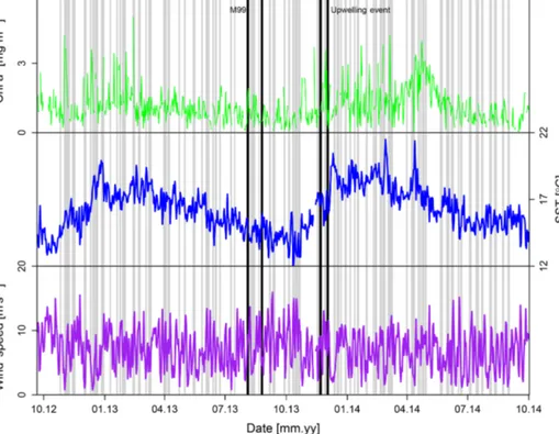
Figure 3.Upwelling events. Surface chlorophylla, temperature, and 10 m wind speed for the Lüderitz domain over the course of the 2-year study period. Days which have been flagged as containing an upwelling event have been shaded. The duration of M99 and the upwelling event discussed in the main text are both demarcated with black rectangles and denoted with a label.

was closer to Lüderitz, the arrival time could be delayed by as much as 50 h, depending on the wind speed and the degree of meandering of the air mass. Back-trajectories implied that despite the high wind speeds usually seen in this coastal zone, significant travel time (1 to 2 d) could be expected for most air masses of interest. As a result, the marine surface flux associated with an atmospheric anomaly could only be said to have taken place within 50 h of its detection. The mag- nitudes of the average atmospheric anomalies and their corresponding flux density estimates are given in Table 1.

3.2 Estimated top-down flux densities

CO2 fluxes were positive for all upwelling events, with an average flux density of 0.70±0.42 µmol m⁻²s⁻¹and a maximum value of 2.0 µmol m⁻²s⁻¹. During upwelling conditions, it is not uncommon to see such strong outgassing of CO2 in a coastal upwelling region; the biological response to new nutrients takes some days to draw down DIC levels (Torres et al., 1999; Loucaides et al., 2012; Cao et al., 2014).

Santana-Casiano et al. (2009) used underway systems on cargo ships and weekly wind speeds to arrive at a mean flux between ca. −0.06 and 0.03 µmol m⁻²s⁻¹for the Lüderitz region, with peak rates as high as 0.06 µmol m⁻²s⁻¹in Au- gust. González-Dávila et al. (2009) found that the Lüderitz region is undersaturated with respect to CO₂, with only upwelled waters seeing oversaturation, with average fluxes on

the order of−0.03±0.3 µmol m⁻²s⁻¹. The flux densities for CO₂reported in this study are not necessarily in conflict with these studies, since a yearly averaged flux density is a different quantity from the event-based flux densities. The impli- cation instead is that flux densities attributed to upwelling events are high enough to contribute significantly to the carbon balance of the Lüderitz and Walvis Bay regions.

Typical O2 flux densities were about −5 µmol m⁻²s⁻¹. The O2flux densities inferred from APO are preferred over those calculated with atmosphericδ(O2/N2), as APO is ex- plicitly formulated to remove land biosphere influences on the relative change in oxygen abundance. A linear regression between the two estimated flux densities yielded a slope of 0.91 and a coefficient of determination of R²=0.98.

The estimated APO flux density was 11 % lower on average than the δ(O₂/N₂)-inferred flux density. That the flux densities for O₂ calculated with these two formulations are close is a good indication that the atmospheric data were primarily influenced by marine fluxes. These are high flux densities for the marine environment; the estimated average flux density for the entire mid-South Atlantic was ∼ 0.03 µmol m⁻²s⁻¹in the inverse modeling study of Gruber et al. (2001) and ca. 0.06 µmol m⁻²s⁻¹in the forward run of a coupled climate and ocean biogeochemistry model of Bopp et al. (2002).

The average flux density attributable to specific upwelling events for N₂O was 0.66±0.4 nmol m⁻²s⁻¹, moderate for a

(9)

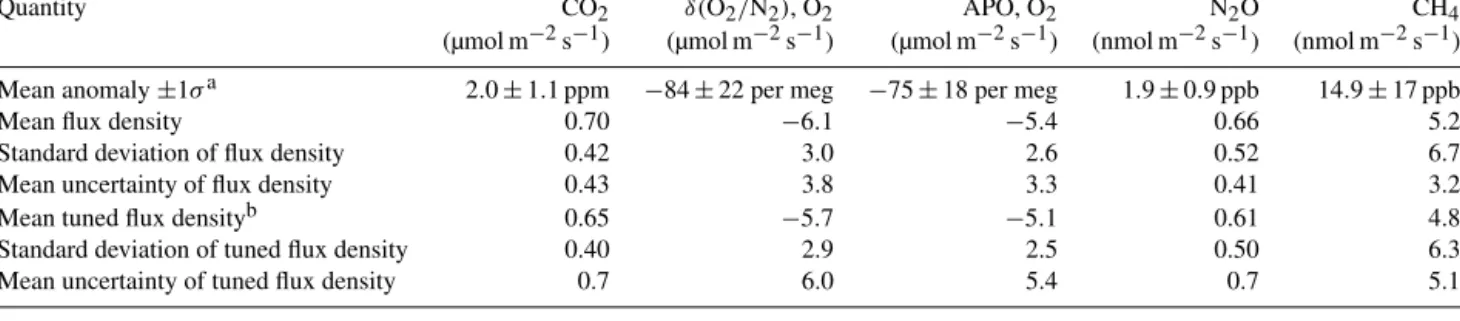
Table 1.Means of all atmospheric anomalies and top-down flux density estimates for identified upwelling events.

Quantity CO2 δ(O2/N2), O2 APO, O2 N2O CH4

(µmol m⁻²s⁻¹) (µmol m⁻²s⁻¹) (µmol m⁻²s⁻¹) (nmol m⁻²s⁻¹) (nmol m⁻²s⁻¹) Mean anomaly±1σ^a 2.0±1.1 ppm −84±22 per meg −75±18 per meg 1.9±0.9 ppb 14.9±17 ppb

Mean flux density 0.70 −6.1 −5.4 0.66 5.2

Standard deviation of flux density 0.42 3.0 2.6 0.52 6.7

Mean uncertainty of flux density 0.43 3.8 3.3 0.41 3.2

Mean tuned flux density^b 0.65 −5.7 −5.1 0.61 4.8

Standard deviation of tuned flux density 0.40 2.9 2.5 0.50 6.3

Mean uncertainty of tuned flux density 0.7 6.0 5.4 0.7 5.1

aFlux density units in the column header correspond to all values except for those in this row.^bThese flux density values are calculated with the value ofqthat results in the best agreement between the top-down flux density and shipboard flux density for the M99 event.

Figure 4.Atmospheric time series at NDAO throughout the upwelling event displayed in Fig. 1. Days flagged as upwelling events are shown as dashed vertical lines.

coastal upwelling system. Flux densities ranged from 0.091–

1.3 nmol m⁻²s⁻¹. From surface data taken on cruise 258 of the RV Africana (Emeis et al., 2018) in the Northern Benguela Upwelling System (NBUS) we estimate a maximum flux density of about 0.07–0.5 nmol m⁻²s⁻¹. Frame et al. (2014) observed flux rates as high as 0.52 nmol m⁻²s⁻¹ in the Cape Frio upwelling cell. The 3-D coupled physical–

biogeochemical model of Gutknecht et al. (2013a, b) pre-

dicts an 8-year mean flux density of 0.02–0.16 nmol m⁻²s⁻¹ for the Walvis Bay region, including both shelf and deeper waters as far west as 10^◦E. The mean flux density of the entire M99 cruise was∼0.03 nmol m⁻²s⁻¹. The model pre- dicts a maximum flux density at the coast (22–24^◦S) of 0.6 nmol m⁻²s⁻¹. Arévalo-Martínez et al. (2019) reported higher N₂O flux densities from a domain encompassing the latitude range of 16–28.5^◦S, ranging between 0.03 and

(10)

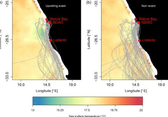
Figure 5.SST during an upwelling event. SST during(a)and preceding and after(b)the upwelling event described in Fig. 2. Five-day back-trajectories calculated for the respective periods are overlain.

1.67 nmol m⁻²s⁻¹. For the Lüderitz–Walvis Bay area they found values similar to this study: up to 0.20 nmol m⁻²s⁻¹.

The moderate, positive CH4 spikes (∼15 ppb) seen during upwelling events corresponded to an average flux density of 5.2 nmol±3.2 m⁻²s⁻¹ and a maximum of 36.4 nmol m⁻²s⁻¹, a high value even for coastal waters.

There are few reported measurements of flux densities or dissolved CH₄ for the Benguela region to place these estimates in context. In what are likely the first measurements of dissolved methane in the Benguela, Scranton and Farring- ton (1977) observed concentrations near Walvis Bay at multiple depths in the 200–900 nM range. The only other available data known to the authors are from cruise 258 of the RV Africanain 2009. These measurements were taken at a vari- ety of depths (up to 400 m) and ranged from 4.7 to 140.0 nM.

Using the nine samples taken from the top 15 m from this cruise, at in situ conditions, a flux of 0.08–1.5 nmol m⁻²s⁻¹ would be expected, from dissolved concentrations ranging from 6.0 to 140 nM. Naqvi et al. (2010) used the data from Scranton and Farrington (1977) and from Monteiro et al.

(2006) to estimate flux densities of 0.03–8.7 nmol m⁻²s⁻¹, the upper end-member of which compares favorably with the rates found in this study for the same ocean region. Though the latter study observed concentrations at a mooring near Walvis Bay as high as 10 µM, these data were from an uncal- ibrated probe and are not usable for a direct comparison to other campaigns. In other EBUS, reported flux densities are much lower.

3.3 M99: atmospheric measurements

Only CO₂ and CH₄were measured continuously in the atmosphere on M99. During the first days of the cruise, before the main upwelling event, a synoptic event brought elevated mixing ratios of CO₂ and CH₄ offshore (Fig. 6). The shipboard measurements of CO₂showed sporadic enhancements relative to the smoothed station background. These enhancements coincided with the regions of higher flux closer to the coast encountered under upwelling conditions (Figs. 6 and 7). In contrast, apart from the initial synoptic event, CH₄was consistently at background levels, usually below the value seen at NDAO. The variability of both species is higher at NDAO than on theMeteorprimarily because NDAO has a strong local wind system which causes diurnal variability in CO2and CH4, as air from the interior is contrasted with marine air brought to the station by the daily sea breeze (Mor- gan, 2015).

3.4 M99: dissolved gas concentrations

All three species measured underway in the water phase showed the largest deviation from atmospheric equilibrium closest to shore (Fig. 7). fCO₂ ranged from 355.5 to 852.3 µatm (87.8 % to 207.3 % saturation), with most of the observed oversaturation occurring under upwelling conditions. Dissolved oxygen was mostly at saturation or slightly above, although close to shore the concentration dropped to a minimum of 180.8 µM (67 % saturation). N₂O surface

(11)

concentrations were rather low for an upwelling region, but agreed well with previously reported values, with the maximum observed concentration of 20.5 nM being comparable to the highest values seen by Frame et al. (2014) for surface measurements in the same region. Recently, Arévalo- Martínez et al. (2019) reported surface N₂O concentrations ranging between 8 and 31 nM for the northern Benguela region. Besides this, the only other in situ measurements of N₂O in the Benguela region known to the authors are in the Marine Methane and Nitrous Oxide (MEMENTO; https:

//memento.geomar.de/de, last access: 28 July 2015) database (Bange et al., 2009; Kock and Bange, 2015), from cruise 258 in 2009 of the RVAfricana. In this dataset, dissolved N2O concentrations for surface waters (the top 15 m) were in the range of 5–51 nM, which brackets the range measured during M99.

The main upwelling event of the cruise, in the Lüderitz–

Walvis Bay cell, began on 4 August 2013 and lasted until 11 August (Fig. 8). Wind speeds declined rapidly after 8 Au- gust. The upwelling event was encountered by the Meteor starting on 8 August, as the vessel reached an upwelling fil- ament, the outer edge of which was subject to net evasion of all three gases (CO₂, O₂, N₂O), likely a result of warming temperatures that would reduce their solubility. The positive flux ratio of O₂:CO₂is generally only produced when ther- mal processes dominate the air–sea flux.

3.5 Comparison of top-down and bottom-up flux density estimates

Due to local wind variability, suitable conditions for detect- ing the upwelling event encountered by theMeteorwere only seen at NDAO on 6, 8, and 10 August 2013. As the vessel was not always in the upwelling cell, only a single atmospheric anomaly at NDAO could be matched to in situ shipboard measurements, namely an anomaly occurring on 10 August. The highest flux rates (positive for CO₂and N₂O, and negative for O₂) were seen within the recently upwelled waters experiencing high wind speeds. Fluxes displayed coupling between all three species, though the area of high flux density for O₂and N₂O was more sharply defined than for CO2.

The top-down estimates agreed reasonably well with the corresponding mean shipboard estimates for a selected 7.5 h period that coincided with the largest flux densities (Fig. 8 and Table 2), but overestimates the flux density relative to the mean shipboard estimate for the flux event. Agreement was best for CO₂, but was as poor as a factor of 3 for N₂O, though given the simplicity of the top-down estimate, this seems fairly reasonable.

The choice of gas transfer velocity parameterization (k_w) was significant in determining the magnitude of the agreement, and the degree of this correspondence between the top- down and shipboard gas transfer velocity-specific estimates varied between species. The cubic relationship of k_McG01

produced higher fluxes during the M99 event and was in bet- ter agreement with the top-down estimate. While this pro- vides a measure of confidence in the top-down flux density estimates, it should be noted that neither of the estimated uncertainties for the top-down or bottom-up approaches ac- counts for errors incurred by the simplifying assumptions within their formulations, and these comparisons should not be considered a “calibration” of the flux determination ork_w parameterization. We suspect that our top-down estimates are overestimates. Cubic relationships with wind speed, derived mostly from eddy covariance data, have not been disproved per se, but after reevaluation of field data (Landwehr et al., 2014), the weight of evidence seems to favor a quadratic relationship (Roobaert et al., 2018), and hence we preferkW14

for comparison.

3.6 Model uncertainty and limitations

The model makes many simplifying assumptions, which we have attempted to incorporate into our uncertainty assumptions. The assumption of a constant boundary layer height, h, is of course not realistic, but we have attempted to ac- count for natural variations in this parameter with our uncertainty range. The uncertainty in the distance traveled de- pends on the accuracy of the back-trajectories, although major errors in transport (e.g., a continental air mass causing the anomaly) are likely to be excluded due to the filtering criteria of the atmospheric record. We also note that the model is sensitive to the dilution rate constant,q, and that this is the parameter we know least well. Previous studies suggest that our in situ determination is reasonable; Price et al. (2004) used multiple species and a model approach to arrive at a mean q of 0.010±0.004 h⁻¹, which is nearly identical to our value of 0.011±0.006 h⁻¹, although the spatial and temporal scale they considered was larger. Dillon et al. (2002) observed rates that were higher for a Sacramento pollution plume, ca. 0.2 h⁻¹.

While we cannot determine for specific events when the simplifying assumptions of the model are problematic, we assume that variations in the dilution rate, the boundary layer height, and errors in transport generally average out and that the estimated average flux from upwelling events is representative. If we “tune” the model by finding the value ofq which results in the value ofF that best matches the M99 event to the kW14 fluxes for each species, we get a lower value of 0.0058±0.007 h⁻¹. Using this value of q, we ob- tain the tuned fluxes reported in Table 2. Though these fluxes have a higher uncertainty associated with them, due to the higher uncertainty inq, we recommend these values, as the top-down and bottom-up comparison suggests that the model overestimates the fluxes.

(12)

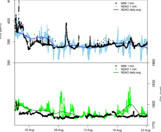
Figure 6.Time series of atmospheric CO₂and CH₄during M99. Atmospheric observations of CO₂and CH₄during the M99 cruise. Black points are the shipboard measurements and colored points are the NDAO measurements. Also shown for both species is a smooth fit to a rolling daily average. The diurnal variability was caused by a sea breeze–land breeze dynamic, with lower CO₂mole fractions and higher CH₄mole fractions occurring at night during the land breeze.

Table 2.Comparisons of top-down and underway flux density estimates for the M99 upwelling event (9 August 2013) Species Unit Top-down Shipboard (k_W14) Shipboard (k_McG01)

CO₂ µmol m⁻²s⁻¹ 0.52±0.3 0.45±0.2 0.67±0.2

δ(O₂/N₂), O₂ µmol m⁻²s⁻¹ −3.4±2 −1.6±0.5 −2.3±0.7

APO, O₂ µmol m⁻²s⁻¹ −2.8±2 −1.6±0.5 −2.3±0.7

N₂O nmol m⁻²s⁻¹ 0.42±0.2 0.15±0.08 0.22±0.1

3.7 Stoichiometry

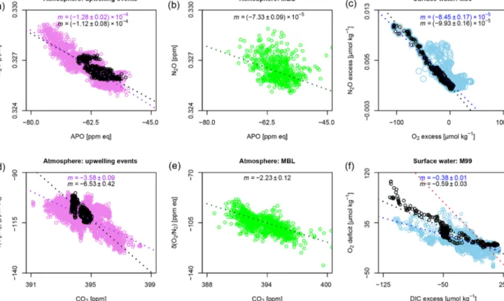
Correlation slopes of atmospheric species can provide fur- ther confidence and insight into source processes if there is an underlying biogeochemical relationship. The well-known inverse relationship between N2O and O2 in the ocean, for instance, is a result of organic matter decomposition and ni- trification (Cohen and Gordon, 1979; Nevison et al., 2003;

Naqvi et al., 2010; Frame et al., 2014). The tight coupling between N₂O and O₂seen in surface concentrations during M99 is preserved during air–sea gas exchange, as these gases behave similarly (Fig. 9). The observed linear correlation in surface waters between these two species is also an indication that intense denitrification was not occurring in the OMZ at the time of sampling, which, if it were taking place, would lead to a breakdown in this relationship at low O₂ (Cohen

and Gordon, 1979). The approximate molar ratio of these two species,−0.8×10⁻⁴to−1×10⁻⁴(N₂O:O₂; mol mol⁻¹), is the same observed by Lueker et al. (2003) for the Trinidad Head region and appears to be a globally consistent value (Nevison et al., 2005; Manizza et al., 2012).

This linear regression slope is often expressed in terms of the excess N₂O (measured N₂O minus N₂O at saturation) and apparent oxygen utilization (saturation minus observed), 1N₂O–AOU in nmol µmol⁻¹. Quantified in this way, it has been used as an estimate of the yield of N₂O as a function of the amount of oxygen consumed (Nevison et al., 2003). However, the relationship is not strictly linear, since N2O production is enhanced at low oxygen levels (Nevi- son et al., 2003; Naqvi et al., 2010; Trimmer et al., 2016).

1N2O–AOU is also sensitive to mixing, as N2O production rates vary widely in the ocean, meaning that the mix-

(13)

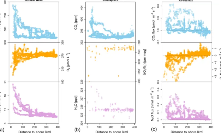
Figure 7.Underway measurements of air–sea fluxes and dissolved concentrations during M99. Dissolved concentrations of CO₂, O₂, and N₂O in surface water, at ca. 6 m depth during M99(a), the atmospheric abundance of all three species(b), and air–sea flux densities for CO₂, O₂, and N₂O withk_W14(c), all as a function of distance from shore. The dashed line in the rightmost panels indicates equilibrium between seawater and the atmosphere (i.e., no flux).

ing of water masses with different compositions can over- whelm the in situ production signal (Suntharalingam and Sarmiento, 2000; Nevison et al., 2003). The 1N₂O–AOU for M99 was 0.088±0.003 nmol µmol⁻¹, with an intercept of 1.6±0.04 nmol and an R²of 0.69. This is a low value, nearly identical to results from the eastern basin of the sub- tropical North Atlantic, where South Atlantic Central Wa- ter is found (Cohen and Gordon, 1979; Suntharalingam and Sarmiento, 2000; Walter et al., 2006), and the eastern equa- torial Atlantic (Arévalo-Martínez et al., 2017). Frame et al.

(2014) showed that most of the N2O in the Benguela Current region is produced in the water column and in the sediment by nitrifier denitrification (Frame et al., 2014). Nevertheless, a substantial portion of this N₂O remains at depth (with a concentration maximum at 200–400 m) and is advected away from the region, without the chance of atmospheric release (Gutknecht et al., 2013b, a; Frame et al., 2014). Hence, the low1N₂O–AOU value found for theMeteorcruise probably reflects both physical and biogeochemical dynamics.

In the case of variations of O₂and CO₂, the stoichiometry of surface waters is not preserved after air–sea exchange, as the majority of carbon is speciated in the carbonate system, and only the portion that remains as dissolved CO₂is available for air–sea gas exchange. This leads to a change

in the ratio, for instance, from 0.58±0.03 in surface waters to−6.53±0.42 in the atmosphere, for the upwelling event encountered during RVMeteor cruise M99 (Fig. 8). These two species can become decoupled through the influences of changing solubility, which would drive evasion of both gases, and net biological production, which would drive evasion of O₂ and invasion of CO₂. These complicating influences are the likely reason for the poorer correlation seen between these two species when compared with N₂O and O₂.

While the top-down flux density estimates cannot be con- firmed with shipboard estimates of flux densities for CH4, it is worth considering that concentrations of methane in bottom waters on the Namibian shelf are likely the highest ever measured in an open coastal system. Values as high as 475 µM in the bottom waters and greater than 5000 µM in sediment porewaters have been observed (Scranton and Far- rington, 1977; Monteiro et al., 2006; Brüchert et al., 2009;

Naqvi et al., 2010). In the water column, the concentration maximum is usually at the seabed or in bottom water, but it is variable and can even occur at 1 m depth (Brüchert et al., 2009). Dissolved methane concentrations are tightly coupled with O₂and show considerable variability, with elevated concentrations being triggered by episodes of hypoxia (Monteiro et al., 2006; Brüchert et al., 2009). The pulse-like nature of

(14)

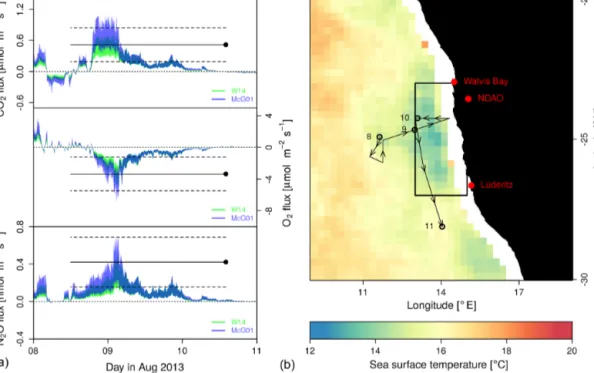
Figure 8.Air–sea flux densities for CO₂, O₂, and N₂O using bottom-up methods(a), with a shaded envelope depicting the estimated surface flux and its uncertainty. Two estimates are shown, each made with a different parameterization forkw. A positive value indicates net evasion.

W14 and McG01 refer to the specific gas transfer velocity parameterization used. The top-down flux density estimate is plotted as a dot at the time of the peak of the associated atmospheric anomaly. The horizontal line extending from each dot represents the time period during which the flux density associated with the anomaly was estimated to have occurred. Dotted lines indicate the uncertainty of the top-down estimate. Grid-cell average TRMM SST data for the 3 d period are overlain with a cruise track and the Lüderitz–Walvis Bay domain(b). The days in August 2013 are marked with labels and open circles on the cruise track.

CH₄in the Benguela region means that the full range of dynamics cannot be captured with a campaign-based sampling approach (Brüchert et al., 2009). What is clear is that there is a tremendous amount of methane production at depth but that the source is variable in strength (Emeis et al., 2004;

Brüchert et al., 2009). Considering the facts that large pockets of free methane gas are contained in the sediment in the Walvis Bay region, craters and pockmarks are known to ex- ist on the seafloor, and bubble streams have been observed coming from the seabed, it seems that there is a possible mechanism by which methane produced in sediments can be abruptly transported to the surface and, hence, avoid oxida- tion (Emeis et al., 2004; Brüchert et al., 2006, 2009). Conse- quently, the Benguela Current is a suspected source of CH4

to the atmosphere, but the amount is ill constrained (Naqvi et al., 2010); Emeis et al. (2018) recently estimated the total annual emission for the entire system to be less than 0.17 Tg CH₄yr⁻¹.

Interestingly, methane was not well correlated with either APO or CO₂in the atmosphere during all upwelling events, suggesting a spatial decoupling (since a cross-correlation analysis indicated this was not a result of lag/temporal decoupling) between methane and these two species. While background observations of CH₄ were generally well correlated with CO₂ and O₂ at NDAO, only some upwelling

events showed such coupling; it seems there is a general relationship between methane and oxygen, but it is not consistent and is occasionally non-existent. Unfortunately, since there are still very few measurements of water-column CH₄ in the Benguela, a full explanation of the methane source remains elusive. From these atmospheric trends it can only be deduced that there is some separate biogeochemical influence on methane that is not exerted over CO₂, O₂, or N₂O.

This observation is arguably consistent with the concept of a dominant sedimentary source of methane that is more lo- calized within the inshore mud belt, where high POC fluxes have created a thick layer of diatomaceous ooze containing free methane gas pockets (Emeis et al., 2004; Brüchert et al., 2006, 2009; van der Plas et al., 2007).

3.8 Regional flux context and future steps

To put our estimated flux densities into the context of regional greenhouse gas budgets, it is necessary to have an approximation of the area involved. For the sake of discussion only, we can very roughly estimate the total annual flux of each species from the Walvis Bay–Lüderitz domain by assuming that grid cells with wind speeds above 3.5 m s⁻¹ and a deseasonalized SST below −0.1^◦C were grid cells with upwelling, that upwelling extends to the coast, and that

(15)

Figure 9.N₂O and O₂variability in the atmosphere and surface water. Comparison of the variability of O₂with respect to N₂O and CO₂ with respect to O₂at NDAO and in surface water. Displayed are the data corresponding to atmospheric anomalies associated with upwelling events(a), of all marine boundary layer air masses as selected by back-trajectories (center), and dissolved concentrations of CO₂, N₂O, and O₂during M99(b). Atmospheric O₂is expressed as APO in ppm equivalents, and dissolved concentrations are expressed as the difference between the measured concentration and the concentration at saturation, i.e., an excess, except for(f), where it is shown as a deficit. In that plot, the Redfield ratio of 1.45 is plotted as a dotted red line for reference. Slopes (m) are given at the top of each plot. The black circles correspond to the upwelling event encountered during M99 (see Fig. 8).

each grid cell with upwelling had the same flux density, i.e., the top-down estimated flux density for a given upwelling event. This approach is very crude and would result in an underestimate, since transport conditions were not always conducive to observing an upwelling event. This would result in annual fluxes of ≥206±151 Gmol yr⁻¹ for CO₂,

≥ −1.6±1.1 Tmol yr⁻¹for O₂,≥272±248 Mmol yr⁻¹for N₂O, and ≥3.3±2.8 Gmol yr⁻¹ for CH₄ from upwelling events.

Such an estimate for CO₂ is substantial when compared to the net flux that Laruelle et al. (2014) estimated of

−424.9 Gmol yr⁻¹ for the entire Benguela region or the

−141.5 Gmol yr⁻¹ found by Gregor and Monteiro (2013) for the southern Benguela. A high flux of CO2is possible due to the higher wind speeds and the more remineralized character of the South Atlantic Central Water that upwells at Lüderitz. Using inverse methods, Gruber et al. (2001) constrained the net flux of oxygen for the temperate South At- lantic (an area of 1.5×10⁷km²) to be 15.5 Tmol yr⁻¹, which suggests that upwelling events in the Lüderitz region could be regionally significant. An annual source of this magnitude

for N₂O is modest when compared to the budgetary calcula- tions of other coastal regions. As the global coastal upwelling source of N₂O is estimated to be 7140 Mmol yr⁻¹(Nevison et al., 2004), the emissions for the Lüderitz–Walvis Bay region would represent 3.2 % of the area but only 1.7 % of these emissions. For CH₄this approximation is 2 to 3 times higher than the net evasion from the Arabian Sea (Bange et al., 1998) and 10 to 20 times greater than the annual release of CH₄ from the entire Mauritanian upwelling system (Kock et al., 2008; Brown et al., 2014), but modest when compared to the estimate of Monteiro (2010) for the entire Benguela Upwelling System, 56 Gmol yr⁻¹, or the 10 Gmol yr⁻¹pro- posed by Emeis et al. (2018) for the NBUS.

A full regional top-down quantification of the annual fluxes – as opposed to the event-based averages we present here – of the Benguela from land-based atmospheric measurements would require additional efforts, such as a Bayesian synthesis inversion of the data, where a prior surface flux field is adjusted to best match the atmospheric observations. This approach relies on an accurate knowledge of atmospheric transport and ideally a dense network of mea-