Oxygenated volatile organic carbon in the western Pacific convective center: ocean cycling, air–sea gas exchange and atmospheric

(1)

https://doi.org/10.5194/acp-17-10837-2017

Oxygenated volatile organic carbon in the western Pacific convective center: ocean cycling, air–sea gas exchange and atmospheric

transport

Cathleen Schlundt^1,a, Susann Tegtmeier², Sinikka T. Lennartz¹, Astrid Bracher^3,4, Wee Cheah^3,b, Kirstin Krüger⁵, Birgit Quack¹, and Christa A. Marandino¹

1Chemical Oceanography Department, GEOMAR Helmholtz Centre for Ocean Research Kiel, Kiel, Germany

2Ocean Circulation and Climate Dynamics, GEOMAR Helmholtz Centre for Ocean Research Kiel, Kiel, Germany

3Climate Sciences, Physical Oceanography of the Polar Seas, Alfred Wegener Institute for Polar and Marine Research, Bremerhaven, Germany

4Institute of Environmental Physics, University of Bremen, Bremen, Germany

5Meteorology and Oceanography Department of Geosciences, University of Oslo, Oslo, 0315, Norway

anow at: Research Center for Environmental Changes, Academia Sinica, Taipei, Taiwan

bnow at: Josephine Bay Paul Center, Marine Biological Laboratory, Woods Hole, MA, USA Correspondence to:Cathleen Schlundt (cschlundt@mbl.edu)

Received: 3 January 2017 – Discussion started: 16 March 2017

Revised: 9 August 2017 – Accepted: 10 August 2017 – Published: 14 September 2017

Abstract.A suite of oxygenated volatile organic compounds (OVOCs – acetaldehyde, acetone, propanal, butanal and butanone) were measured concurrently in the surface water and atmosphere of the South China Sea and Sulu Sea in Novem- ber 2011. A strong correlation was observed between all OVOC concentrations in the surface seawater along the entire cruise track, except for acetaldehyde, suggesting similar sources and sinks in the surface ocean. Additionally, several phytoplankton groups, such as haptophytes or pelagophytes, were also correlated to all OVOCs, indicating that phytoplankton may be an important source of marine OVOCs in the South China and Sulu seas. Humic- and protein-like fluorescent dissolved organic matter (FDOM) components seemed to be additional precursors for butanone and acetaldehyde. The measurement-inferred OVOC fluxes generally showed an uptake of atmospheric OVOCs by the ocean for all gases, except for butanal. A few important exceptions were found along the Borneo coast, where OVOC fluxes from the ocean to the atmosphere were inferred. The atmospheric OVOC mixing ratios over the northern coast of Borneo were relatively high compared with literature values, suggesting that this coastal region is a local hotspot for atmospheric OVOCs. The calculated amount of OVOCs entrained into

the ocean seemed to be an important source of OVOCs to the surface ocean. When the fluxes were out of the ocean, marine OVOCs were found to be enough to control the lo- cally measured OVOC distribution in the atmosphere. Based on our model calculations, at least 0.4 ppb of marine-derived acetone and butanone can reach the upper troposphere, where they may have an important influence on hydrogen oxide rad- ical formation over the western Pacific Ocean.

1 Introduction

Oxygenated volatile organic compounds (OVOCs) are com- prised of ketones, aldehydes and alcohols. They are ubiqui- tous throughout the troposphere, where they influence the ox- idative capacity and air quality. OVOCs, such as acetone and acetaldehyde, affect the cycling of reactive nitrogen compounds, such as nitrogen oxide (NO) and nitrogen dioxide (NO₂), and associated ozone production. They are also in- volved in the production of peroxynitric acid (HNO₄), and nitric acid (HNO₃), and they are precursors of peroxyacetyl nitrate (PAN), a persistent harmful pollutant (Folkins and Chatfield, 2000; Fischer et al., 2014). OVOCs, such as ace-

(2)

tone, are a source of hydrogen oxide radicals (HOx), which is of special importance for the upper troposphere (UT), where the concentration of a main precursor, namely water vapor, is much lower than at the Earth surface (Singh et al., 1995;

Wennberg et al., 1998; Müller and Brasseur, 1999). Further- more, OVOCs, such as acetone, acetaldehyde and propanal, can contribute to particle formation in the atmosphere, resulting in albedo enhancement (Blando and Turpin, 2000).

The distribution of OVOCs in the atmosphere is determined by a variety of different sources and sinks. Terrestrial emissions from living and decaying plants and the oxidation of hydrocarbons in the atmosphere are believed to be the main sources of atmospheric OVOCs, such as methanol and acetone. Additionally, biomass burning and anthropogenic emissions play a crucial role for the atmospheric OVOC cycle. Atmospheric sinks of OVOCs include photolysis, oxidation, and their dry and wet deposition over land and ocean (Heikes et al., 2002; Jacob et al., 2002, 2005). Based on measurements and model calculations, the strength of atmospheric OVOC sources and sinks is still unbalanced, indicating that unknown global sources and sinks of OVOCs exist (Singh et al., 2003; Jacob et al., 2002). It is believed that the ocean plays a crucial role for atmospheric OVOC concentrations; however, it is still poorly understood how the ocean impacts the atmospheric OVOC budget (Heikes et al., 2002;

Mincer and Aicher, 2016; Williams et al., 2004). The main production pathway of OVOCs in the ocean seems to be the photochemical and/or photosensitized oxidation of dissolved organic matter (DOM) in the surface ocean followed by rapid consumption by bacteria (Mopper and Stahovec, 1986; Beale et al., 2013; de Bruyn et al., 2013, 2011; Dixon et al., 2013).

The production of OVOCs by specialized bacteria or picophytoplankton seems to be a rather minor source in the ocean (Nemecek-Marshall et al., 1995; Nuccio et al., 1995; Sunda and Kieber, 1994). Oceanic sinks of OVOCs are their photochemical destruction, air–sea gas exchange or turbulent mixing into the deep ocean (Carpenter et al., 2012).

It is still debated whether the ocean is a net source or sink for atmospheric OVOCs, given that studies have shown con- trasting results. For instance, direct flux measurements of acetone in distinct oceanic regions showed that the North Pacific and North Atlantic Ocean were sinks for acetone, while the subtropical Atlantic was observed to be a source and the South Atlantic was a net zero flux region. Addi- tionally, global flux estimations, when averaged and scaled to the global ocean, showed a wide range between−48 to

−1 Tg yr⁻¹(Marandino et al., 2005; Yang et al., 2014a), with the negative values here reflecting the ocean as a sink for acetone. The ocean appears to be a source of acetaldehyde, with an estimated global flux ranging from 3 to 175 Tg yr⁻¹, based on model calculations and direct flux measurements (Beale et al., 2013; Millet et al., 2010; Singh et al., 2004; Yang et al., 2014a). Model calculations suggest that the Pacific Ocean is a source of propanal, contributing 45 Tg yr⁻¹ to the atmosphere (Singh et al., 2003). To the best of our knowledge,

no ocean–atmosphere butanal or butanone fluxes have been reported to date.

When OVOCs are emitted from the ocean into the marine boundary layer (MBL), they can be destroyed by photochemical processes, deposit back to the surface, accumu- late in the MBL, or be redistributed by deep convection into the mid- and upper troposphere throughout the year (Apel et al., 2012). The latter possibility would lead to an UT source of HO_x. The location of this study, the tropical west Pacific, is of special importance in this case, as it is an effective en- trance region of trace gases into the UT and lower stratosphere due to frequent deep convection (e.g., Aschmann et al., 2009). Even short-lived substances, such as dimethyl- sulfide (DMS) or methyl iodide with lifetimes of hours to days, can be entrained into the tropical tropopause layer and can reach the lower stratosphere here (Tegtmeier et al., 2013;

Marandino et al., 2013).

We present the first study of the distribution of a suite of OVOCs (acetaldehyde, acetone, propanal, butanal and butanone) in the surface ocean and atmosphere in the most western region of the Pacific Ocean, the South China Sea and the Sulu Sea, measured in November 2011. In past studies, OVOCs were generally measured either exclusively in the ocean or in the atmosphere (Dixon et al., 2011; Elias et al., 2011; Singh et al., 2001). Only a few studies have measured acetaldehyde and acetone simultaneously in the water and air (Marandino et al., 2005; Yang et al., 2014a, b). However, the transport and distribution of the oceanic OVOCs in the upper troposphere has never been investigated. We present a comprehensive study of the potential controls on the distribution of OVOCs in the surface ocean, their air–sea flux, and their horizontal and vertical atmospheric transport over the western Pacific Ocean. Additionally, the possible influence of OVOCs on atmospheric chemistry in the UT is discussed.

2 Methods, data analysis and model 2.1 Sampling site

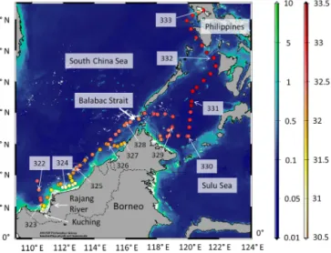
During the SHIVA (Stratospheric ozone: Halogen Impacts in a Varying Atmosphere) cruise from Singapore (15 Novem- ber 2011) to Manila (29 November 2011), the German R/V Sonnecrossed the southern South China Sea, along the north- western coast of Borneo, and entered the Sulu Sea through the Balabac Strait (Fig. 1). Northeasterly trade winds (the median of the wind direction: 50–60^◦), with a mean wind speed of 5.8±2.9 ms⁻¹, prevailed during the cruise. The observed mean surface air temperature of 28.3±0.8^◦C was on average 0.8±0.8^◦C below the sea surface temperature with a mean of 29.2±0.5^◦C, benefiting convective activity and precipitation events. The distinct transport of water vapor to the mid-troposphere was seen in elevated humidity up to about 6 km, which did not coincide with the marine boundary layer height of 420±120 m, reflecting the characteristics

(3)

Figure 1.Cruise track (17–29 November 2011) showing salinity in the surface seawater at each point when an underway measurement was conducted. Numbers show the day of the year and the arrows the location when a day started. Background colors show chloro- phylla(Chla; level-2) data from the MERIS satellite sensor (onboard Envisat) using the polymer product (Steinmetz et al., 2011).

Note that the Chlaconcentrations are shown on a logarithmic scale.

of an unstable, convective, well-ventilated tropical boundary layer. A detailed overview of the SHIVA campaign is given by Fuhlbrügge et al. (2016).

2.2 OVOC measurements

Oceanic samples (n=90) were collected from day of year (DOY) 321.9, corresponding to 3.63^◦N and 110.34^◦E, and atmospheric samples (n=37) were collected from DOY 325.3 and 4.6^◦N and 113.1^◦E (Fig. 1).

The samples were analyzed for ethanal (acetaldehyde, CH₃CHO), propanone (acetone, (CH₃)₂CO), propanal (propionaldehyde, CH₃CH₂CHO), butanal (butyraldehyde, CH₃(CH₂)₂CHO) and butanone (methyl ethyl ketone, CH₃C(O)CH₂CH₃)using a purge and trap system coupled to a gas chromatograph and a mass spectrometer (GC-MS;

GC: Agilent Technologies, 7890A; MS: Agilent Technolo- gies, 5975C MS, single quadrupole).

Oceanic samples were taken from an underway pumping system installed in the hydrographic shaft (6 m depth) ev- ery 3 h. The samples were collected bubble free in 250 mL glass bottles sealed with gastight Teflon (PTFE)-coated lids and were measured immediately after sampling. For each sample, 10 mL of unfiltered seawater was transferred from the sampling bottle into the purge chamber using a gastight syringe. OVOCs were expelled from the seawater with a helium flow of 20 mL min⁻¹ for 20 min and were trapped in 1/16 inch Sulfinert^® stainless steel tubing submerged in liquid nitrogen. Potassium carbonate (K₂CO₃) within a 9 cm length glass tube, 0.5 cm in diameter, was used as a

moisture trap. We flushed the K2CO3 for 20 min with helium (80 mL min⁻¹)prior to use to avoid contamination with OVOCs. We obtained good reproducibility of OVOC measurements when the moisture trap was replaced after five measurements. Hot water was used to transfer the trapped OVOCs on the GC column (fused silica capillary column Supel-QTM Plot, 30 m×0.32 mm) ending in the MS. Wa- ter standards were prepared by injecting liquid OVOCs into pure 18 MMilli-Q water and were measured in the same way as water samples. The mean analytical errors of the water samples were as follows: acetaldehyde – 4.9 %; acetone – 20.9 %; propanal – 13.3 %; butanal – 12.8 %; and butanone – 7.8 %. The reproducibility of the system for the water measurements was 20 %. The lower detection limit of all OVOCs was around 0.06 nmol L⁻¹.

Due to the high solubility of OVOCs in water, it was not possible to expel the gases entirely from the water. Thus, we adjusted all parameters influencing the purge procedure, such as water temperature of the purge chamber (30^◦C), helium gas flow (20 mL min⁻¹)and purging time (20 min), to ensure the reproducibility of the purging procedure between calibra- tions and samples.

Atmospheric samples were taken in conjunction with water samples from the bow of the ship (about 10 m above seawater surface) by using a portable pump and trap system. Air was pumped for 10 min with a flow of 80 mL min⁻¹through a K2CO3moisture trap and was concentrated in a Sulfinert^® stainless steel tube submerged in liquid nitrogen. We did not sample at the bow of the ship if the relative wind direction was circulating or coming from aft to avoid contamination of our samples by ship emissions. After trapping, the sample tubing was immediately connected to the GC-MS to avoid loss of sampled compounds. The air samples were transferred to the GC-MS using hot water and were measured in the same way as the water samples. A gas standard mixture of acetaldehyde, acetone, propanal, butanal and butanone in nitrogen (all at mixing ratios of 1 ppm, produced by Apel- Riemer, USA) was trapped and measured in the same way as air samples. The mean analytical errors of the atmospheric samples were as follows: acetaldehyde – 6.3 %; acetone – 13.5 %; propanal – 14.2 %; butanal – 18.7 %; and butanone – 12.5 %. The reproducibility of the system for the air measurements was 10.5 %.

2.3 Phytoplankton pigment analysis

Water samples for phytoplankton pigment analysis were taken from the underway pump system and from Niskin bottles attached to a rosette equipped with a conductivity, temperature and depth sensor (CTD). The samples were filtered through Whatman GF/F filters (0.7 µm pore size) and were immediately shock frozen in liquid nitrogen and stored at −80^◦C on board. Pigment extraction and analysis were done in the laboratory at the Alfred Wegener In- stitute using the high-performance liquid chromatography

(4)

(HPLC) technique according to the method of Barlow et al. (1997), and they were modified as described in Taylor et al. (2011). In brief, filtered samples were extracted in 1.5 mL of 100 % acetone plus 50 µL canthaxanthin as an in- ternal standard solution and analyzed by HPLC using a Wa- ters 717plus autosampler, a Waters 600 controller, an LC Mi- crosorb C8 column and a Waters 2998 photodiode array de- tector. Part of the pigment data have been reported in Soppa et al. (2014), and all data are available in the PANGAEA database (https://doi.org/10.1594/PANGAEA.848589).

Based on the pigment concentrations, the corresponding major phytoplankton groups were calculated using the CHEMTAX software (version 1.95; Mackey et al., 1996), which employs a “steepest descent” algorithm to optimize the marker pigments to chlorophyll a (Chla) ratios identified from HPLC to a given input matrix. Five input ratio matrices from the Pacific region were chosen as seed values (DiTullio et al., 2003; Higgins and Mackey, 2000; Zhai et al., 2011; Miki et al., 2008; Mackey et al., 1996). For each seed ratio matrix, 16 pigment ratios were randomly generated following the method of the software provider (Wright et al., 2009). Each of the randomly generated pigment ratios was then used as a starting value for CHEMTAX analysis.

Six output matrices with the lowest root mean square error were averaged and used as the “final” starting ratios. A total of nine phytoplankton groups, namely, diatoms, dinoflagellates, haptophytes, prasinophytes, chlorophytes, chryso- phytes, pelagophytes, prochlorophytes and cyanobacteria (excluding prochlorophytes), were determined. Good agreement with significant correlations (Pearson correlation with correlation coefficientr)was observed between five taxa derived from CHEMTAX and from microscopic and flow cy- tometry analysis of the same water samples. The correlations are r=0.4 (prochlorophytes), r=0.67 (Synechococ- cussp.),r=0.75 (coccolithophores (haptophytes)),r=0.93 (dinoflagellate) andr=0.95 (diatoms).

2.4 Nutrient measurements

Dissolved nutrients (phosphate, silicate, nitrate, nitrite) were measured photochemically with a QuAAtro auto- analyzer (SEAL Analytical, UK) according to the method of Grasshoff et al. (1999).

2.5 Fluorescent dissolved organic matter (FDOM) analysis

Excitation emission matrices (EEMs) were measured with an F-2700 FL spectrophotometer (Hitachi) over an excitation range of 250 to 500 nm and an emission range of 280 to 600 nm (both with a 5 nm sampling interval) using a 1 cm quartz cuvette. The slit width was set to 10 nm for both.

EEMs were blank subtracted and Raman normalized and are reported here in Raman units (RU). A parallel factor analysis (PARAFAC) was performed for 187 EEMs using the drEEM

toolbox (Murphy et al., 2013) for MATLAB. Six components were split half-validated using alternating initialization.

2.6 Statistics

We applied principal component analysis (PCA) to examine how a combination of different physical, chemical and biological variables, such as the phytoplankton community, nutrient availability or physical parameters (temperature, salinity), might influence the OVOC concentration and distribution in the surface seawater of the South China Sea and Sulu Sea. We calculated PCA to reveal a simplified under- lying structure of our multivariate dataset and to find the best model explaining the variance in our data. PCA converts a large number of variablesninto a smaller number of artificial variablesq (principal components, PCs;n>q)with a mini- mum loss of information. Prior to the PCA, we normalized our dataset to compare data with different units. Each PC has an associated eigenvalue, which indicates the variation in the data. The higher the eigenvalue the better the variation in all the data is explained by the appropriate PC. Furthermore, the factor loadings of the PCs were calculated, which explain the variance in each variable by the corresponding PC. High factor loadings refer to high and significant correlations between variables. In addition to the PCA, we applied the Spearman rank correlation analysis (with the correlation coefficientr_s) to find possible direct links between the different OVOCs.

2.7 Flux calculations

The oceanic and atmospheric OVOC data were used for flux calculations. Wind speed and sea surface temperature obtained from ship sensors at 10 min resolution were selected for time and positions of OVOC measurements. The flux (F) was calculated according to Johnson (2010):

F = −K_a(C_a−K_HC_w). (1)

K_a is the total transfer velocity from the gas phase point of view that is composed of the water-side single-phase transfer velocity (k_w)and the air-side single-phase transfer velocity (k_a; Johnson, 2010). Note that according to Eq. (1), a negative flux reflects a flux from the atmosphere to the ocean and vice versa. The 10 m height wind-speed-dependentkw

determined by Nightingale et al. (2000) was adjusted with the temperature-dependent Schmidt number for CO2that we corrected with the molar volume of each OVOC, according to Hayduk and Laudie (1974). We used thekadetermined by Duce et al. (1991), which depends on the wind speed at 10 m height and on the molecular weight of the trace gas. John- son (2010) provided a discussion of using Duce et al. (1991) to compute k_a. Therefore, we used the k_a parameterization of Mackay and Yeun (1983) to recompute the OVOC fluxes.

The newly computed fluxes were on average 20 % higher for positive fluxes and around 20 % lower in the case of negative fluxes, resulting in a higher amount of OVOC concentrations

(5)

exchanged between the ocean and the atmosphere in both di- rections. We treated this difference in the calculated fluxes as uncertainty and used the previous fluxes determined by using the Duce et al. (1991) parameterization ofk_aas a con- servative estimate of OVOC fluxes into and out of the ocean surface.

C_a andC_w are the concentrations of OVOCs in the atmosphere (around 10 m above sea level) and in the sea surface water (6 m depth), respectively.K_His the dimensionless, temperature-dependent Henry’s law constant, which was described in Sander (1999) and which was modified for each OVOC by using empirically determined apparent partition coefficients for the different OVOCs from Zhou and Mop- per (1990).

2.8 OVOC atmospheric transport modeling

The atmospheric transport of the OVOCs from the oceanic surface into the MBL was simulated with the Lagrangian particle dispersion model FLEXPART (Stohl et al., 2005).

FLEXPART is an off-line model driven by external meteo- rological fields and includes parameterizations of moist convection and turbulence in the boundary layer as well as emissions, dry deposition, scavenging and chemical decay of atmospheric tracers. This model has been validated extensively with measurements from large-scale tracer experiments and has been used in many studies of long-range and mesoscale transport (Stohl et al., 2005 and references therein).

For the simulations of the atmospheric transport and chemical decay of the emitted oceanic OVOCs, we calculated trajectories of a multitude of air parcels. For each data point of the observed sea-to-air flux, 10 000 air parcels were released from a 0.1^◦×0.1^◦grid box at the ocean surface centered on the measurement location and loaded with the amount of the OVOCs prescribed by the observed emissions at this location. The air parcels were released over a time period ranging between 1 and 18 days depending on the chemical lifetime of the respective gas as given below. The FLEXPART v9.2 runs were driven by the ECMWF reanalysis ERA-Interim (Dee et al., 2011) given at a horizontal resolution of 1^◦×1^◦ on 60 model levels. FLEXPART calculates transport, dispersion and convection of the air parcels from the horizontal and vertical wind fields, temperature, specific humidity, convective and large-scale precipitation. The chemical decay of the OVOCs was prescribed by their atmospheric lifetime, which was set to 14 h for butanal (Calvert, 2011), 15 h for propanal (Rosado-Reyes and Francisco, 2007), 1 day for acetaldehyde (Millet et al., 2010), 10 days for butanone (Calvert, 2011) and 18 days for acetone (Khan et al., 2015). A second set of simulations was conducted to analyze possible sources of the observed atmospheric mixing ratios. While the importance of the emissions was investigated by forward runs as described above, possible sources of the observed mixing ratios were identified by backward trajectory runs. At each measurement

location, 100 trajectories were released at the time of the observation and calculated backward in time over a 24 h period.

3 Results and discussion 3.1 OVOCs in the surface ocean

For the first time, a suite of OVOCs were measured in the surface water of the southern part of the South China Sea and adjacent Sulu Sea and in the overlying marine boundary layer. Over the entire cruise track, average surface seawater concentrations (6 m depth) for acetaldehyde, acetone, propanal, butanal and butanone were 4.1, 21.3, 1, 0.7 and 0.9 nmol L⁻¹, respectively (Table 1). Acetaldehyde concentrations were similar to previous measurements in the surface waters of the open Atlantic and Pacific oceans (Beale et al., 2013; Kameyama et al., 2010; Mopper and Stahovec, 1986; Yang et al., 2014a; Zhou and Mopper, 1997) and in the lower range compared to coastal concentrations in the En- glish Channel (Beale et al., 2015; Table 2). In contrast, the concentration of acetone was in the higher range compared to literature values of the open-ocean and coastal regions (Beale et al., 2013, 2015; Dixon et al., 2014; Kameyama et al., 2010; Marandino et al., 2005; Williams et al., 2004; Yang et al., 2014a, b; Zhou and Mopper, 1997). Only a few studies measured propanal, butanal and butanone in the ocean.

The concentrations in our study were elevated compared to a study in the open ocean near the Bahamas by Zhou and Mop- per (1997) and low compared to a study in the coastal waters of southeast Florida (Mopper and Stahovec, 1986; Table 2).

Corwin (1969) measured the same suite of OVOCs as in our study in the Straits of Florida and in the Eastern Mediter- ranean. Their concentrations were 1 to 3 orders of magnitude higher compared to our values and to literature values listed in Table 2.

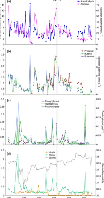
The distribution pattern of the OVOCs was variable in the shallow ocean along the coast off Borneo in the South China Sea (Fig. 2a, b; DOY 323–329, < 117^◦E) and showed mainly low concentrations in the open ocean of the Sulu Sea and in the coastal region off the eastern Philippines (Fig. 2a, b;

DOY 329–333, > 117^◦E). Slightly elevated OVOC concentrations occurred close to the coast off Kuching (Fig. 2a, b;

DOY 322–323) in conjunction with elevated nitrate and total Chla concentrations (Figs. 1 and 2d). The rivers Sadong, Lupar and Saribas form a large river delta to the east of Kuching that impacts the coastal region. This was visible in a decrease in salinity and slightly elevated nutrient concentrations, indicated by nitrate in Fig. 2d, due to river outflow that consequently induced a phytoplankton bloom. Elevated OVOC concentrations occurred also around 5^◦N and 114^◦E (Fig. 2a, b; DOY 325) and at the northern tip of Borneo (Fig. 2a, b; DOY 328–329, between 7–8^◦N and 117–119^◦E).

These two regions were less influenced by river outflow, as

(6)

Table 1.Averages and ranges of water and air concentrations of OVOCs and their air–sea gas exchange rates. Negative flux values refer to gas exchange from the atmosphere into the ocean.

Water Air Flux

Median Range Median Range Median Range

(nmol L⁻¹) (ppb) (µmol m⁻²d⁻¹)

Acetaldehyde 4.11 0.35–14.45 0.86 0.11–8.5 −10.11 −139.36–7.27 Acetone 21.33 2.47–67.76 2.1 0.14–14.48 −18.34 −166.14–30.63

Propanal 1.04 0.08–3.29 0.15 0.01–1.42 0.03 −7.49–2.58

Butanal 0.71 < 0.06–3.35 0.06 0.006–1.21 0.5 −6.56–2.99

Butanone 0.88 0.11–4.31 0.06 0.003–35.46 −0.71 −344.82–1.96

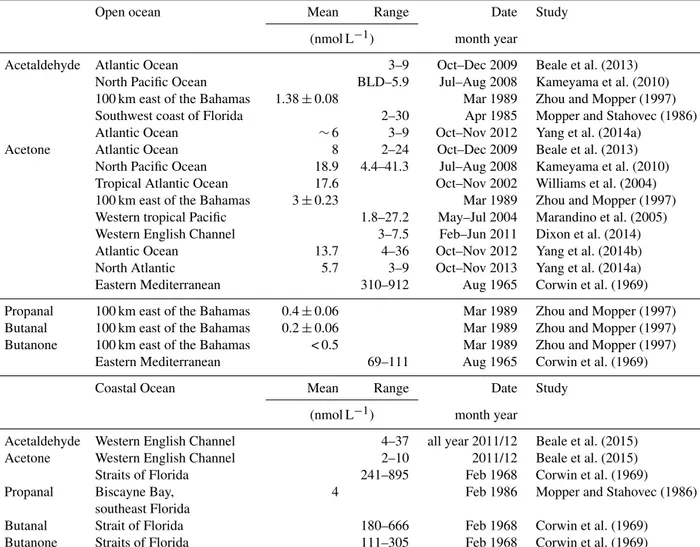
Table 2.Literature values of OVOCs in the open and coastal oceans. BLD: below limit of detection.

Open ocean Mean Range Date Study

(nmol L⁻¹) month year

Acetaldehyde Atlantic Ocean 3–9 Oct–Dec 2009 Beale et al. (2013)

North Pacific Ocean BLD–5.9 Jul–Aug 2008 Kameyama et al. (2010)

100 km east of the Bahamas 1.38±0.08 Mar 1989 Zhou and Mopper (1997) Southwest coast of Florida 2–30 Apr 1985 Mopper and Stahovec (1986)

Atlantic Ocean ∼6 3–9 Oct–Nov 2012 Yang et al. (2014a)

Acetone Atlantic Ocean 8 2–24 Oct–Dec 2009 Beale et al. (2013)

North Pacific Ocean 18.9 4.4–41.3 Jul–Aug 2008 Kameyama et al. (2010) Tropical Atlantic Ocean 17.6 Oct–Nov 2002 Williams et al. (2004) 100 km east of the Bahamas 3±0.23 Mar 1989 Zhou and Mopper (1997) Western tropical Pacific 1.8–27.2 May–Jul 2004 Marandino et al. (2005) Western English Channel 3–7.5 Feb–Jun 2011 Dixon et al. (2014)

Atlantic Ocean 13.7 4–36 Oct–Nov 2012 Yang et al. (2014b)

North Atlantic 5.7 3–9 Oct–Nov 2013 Yang et al. (2014a)

Eastern Mediterranean 310–912 Aug 1965 Corwin et al. (1969)

Propanal 100 km east of the Bahamas 0.4±0.06 Mar 1989 Zhou and Mopper (1997) Butanal 100 km east of the Bahamas 0.2±0.06 Mar 1989 Zhou and Mopper (1997) Butanone 100 km east of the Bahamas < 0.5 Mar 1989 Zhou and Mopper (1997)

Eastern Mediterranean 69–111 Aug 1965 Corwin et al. (1969)

Coastal Ocean Mean Range Date Study

(nmol L⁻¹) month year

Acetaldehyde Western English Channel 4–37 all year 2011/12 Beale et al. (2015)

Acetone Western English Channel 2–10 2011/12 Beale et al. (2015)

Straits of Florida 241–895 Feb 1968 Corwin et al. (1969)

Propanal Biscayne Bay, southeast Florida

4 Feb 1986 Mopper and Stahovec (1986)

Butanal Strait of Florida 180–666 Feb 1968 Corwin et al. (1969)

Butanone Straits of Florida 111–305 Feb 1968 Corwin et al. (1969)

indicated by elevated salinity and lower nutrient concentrations compared to the region west of 114^◦E.

We correlated the OVOCs to each other to find possible relationships between them. Significant correlations were found between all OVOCs (up to r_s=0.8, p value 0.001).

However, the coefficient of determination was relatively low (r_s=0.45–0.55,pvalue 0.001) for correlations between ac-

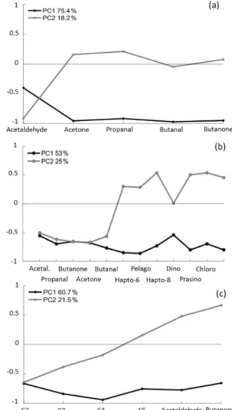
etaldehyde and the other OVOCs. Additionally, we examined the relationships between the OVOCs for the entire cruise track using PCA. Overall, 75 % of the OVOC variability was explained by the first component of the PCA (Fig. 3a), which points to their similar distribution pattern and their close relationship. When acetaldehyde was excluded from the PCA model, 89 % of the variability in the remaining OVOCs was

(7)

Figure 2.OVOC concentrations (a, b) in water,cthe phytoplankton groups pelagophytes, haptophytes (mainlyPhaeocystissp.) and prasinophytes, d nitrate, total chlorophyll a(TChla) and salinity plotted against the day of the year (DOY). The location of the data points can be deduced from Fig. 1. The vertical line shows the location of the Balabac Strait (117^◦E), where coastal conditions changed to open-ocean conditions.

explained by the first component. It seems that acetaldehyde was controlled by additional factors to the other OVOCs in the South China Sea and Sulu Sea. Several studies investigated the biogeochemical pathways of acetaldehyde and acetone in different oceanic regions. For instance, de Bruyn et al. (2011) observed higher production rates for acetaldehyde compared to acetone from photochemical oxidation of colored dissolved organic matter (CDOM) in a coastal region of

southern California, USA. In contrast, Dixon et al. (2013) estimated a higher photochemical production rate for acetone compared to acetaldehyde and showed that up to 13 % of acetone and up to 100 % of acetaldehyde were lost in the surface water of the Atlantic Ocean due to microbial oxidation.

Furthermore, they estimated a biological lifetime for acetone and acetaldehyde of between 5 and 80 days and between 2 h and 1 day, respectively. Dixon et al. (2014) confirmed that bacteria preferred acetaldehyde rather than acetone as carbon or energy sources in the English Channel. Mopper and Stahovec (1986) observed a stronger diurnal cycle with the highest concentrations in the late afternoon for acetaldehyde compared to acetone. Additionally, Beale et al. (2013) sug- gested that regions of the Atlantic Ocean might be under- saturated in acetaldehyde but not in acetone. It seems that acetaldehyde is subject to a faster turnover compared to acetone. This might explain the weaker link between acetaldehyde and acetone, and probably also with the other OVOCs, in this study.

3.1.1 OVOC concentrations influenced by phytoplankton and FDOM

We applied PCA to understand which environmental factors (nutrients, phytoplankton pigments, biomasses of phytoplankton groups, phytoplankton cell size, salinity, temperature, wind speed, halogenated compounds, different FDOM components and methane) might be related to or influence the OVOCs at the sampling site. We found a link between the OVOCs and several phytoplankton groups, including haptophytes, pelagophytes, dinoflagellates, prasinophytes and chlorophytes (Fig. 3b), all of which made up 37 % biomass on average over the cruise. In total, 53 % of the variability in the OVOCs together with these phytoplankton groups was accounted for by the first component of the PCA. The link between the OVOCs and phytoplankton can either refer to the direct production of OVOCs by phytoplankton or to similar environmental conditions causing the same variability for both. However, it is unlikely that, over the entire cruise track, in both coastal and open-ocean regions, the same environmental conditions prevailed that triggered the same OVOC and phytoplankton distribution pattern without any direct connection between the two. We concluded, based on the PCA results, that it is possible that phytoplankton was a source of OVOCs in the South China Sea and Sulu Sea.

To the best of our knowledge, no study has described the direct production of OVOCs by phytoplankton. Whe- lan et al. (1982) tested both macroalgae and phytoplankton for OVOC production and measured high concentrations of OVOCs (acetone, propanal, butanal and butanone) only in macroalgae but not in phytoplankton, such as diatoms, dinoflagellate and haptophytes, therefore excluding phytoplankton as OVOC producers. Additionally, Beale et al. (2013) found no correlation between acetone production and primary production in the Atlantic Ocean and, thus, ex-

(8)

Figure 3.Principal component analysis (PCA) of OVOCs in seawater (a); between OVOCs in seawater and phytoplankton (b);

and between fluorescent dissolved organic matter (FDOM) groups, acetaldehyde and butanone in seawater (c). Numbers on the y axes indicate the factor loadings of each variable of each principal component (PC). The percentages show the explained variability in the dataset by each PC. Hapto-6: haptophytes, mainly coccolithophorids; Pelago: pelagophytes; Hapto-8: haptophytes, mainly Phaeocystis sp.; Dino: dinoflagellates; Prasino: prasinophytes; Chloro: chlorophytes.

cluded marine phytoplankton as a significant source of acetone. Nuccio et al. (1995) tested axenic monocultures of cyanobacteria and dinoflagellates for their ability to produce acetaldehyde and propanal. They mainly observed the production of formaldehyde in these cultures. However, a filtered (0.2 µm pore size) seawater sample with a natural as- semblage of bacteria and picoplankton showed an increase in propanal concentration together with Chl a concentration, assuming propanal production by picophytoplankton or their symbiotic bacteria. In addition, Sinha et al. (2007) ob-

served significant correlations of the haptophyteEmiliania huxleyi and picophytoplankton with acetone and acetaldehyde emissions in a mesocosm study in Norway, suggesting a possible production of OVOCs by phytoplankton. Min- cer and Aicher (2016) showed that a broad range of marine phytoplankton species of different groups produce significant amounts of methanol, the most abundant OVOC in the atmosphere. Comprehensive studies are lacking that test a wide range of phytoplankton species for their potential to produce different OVOCs.

If the OVOCs in this study were not produced by phytoplankton, it is possible that they were produced by attached or symbiotic bacteria of the phytoplankton. Several studies showed that marine bacteria can produce acetone, acetaldehyde and, most likely, propanal (Nemecek-Marshall et al., 1995, 1999; Nuccio et al., 1995; Sunda and Kieber, 1994).

However, measurements of bacteria cell abundance and com- position are not available for our study. Thus, incubation experiments have to be conducted in the future to test directly the microbial production and consumption of OVOCs in the ocean.

An additional main source of OVOCs in surface seawater is the DOM pool (Mopper and Stahovec, 1986; Zhou and Mopper, 1997). DOM is composed of non-colored and colored DOM that can be further subdivided into a fluorescent part of the CDOM pool, called FDOM. We identified six FDOM components in our study, with four humic-like substances (component C2–C4, C6), which were composed of refractory humic-like compounds that originated from coastal and terrestrial environments and which were either soil-derived, segregated by marine algae or altered by microbial activities (C2 described in Tanaka et al., 2014, as C1 and in Yu et al., 2015, as C5; C3 described in Li et al., 2015, as C4; C4 described in Kowalczuk et al., 2009, as C2; C6 described in Kowalczuk et al., 2013, as C5). Furthermore, two protein-like substances (C1 and C5) were identified, originat- ing from marine environments associated with recent biological production in surface seawater (C1 described in Kowal- czuk et al., 2013, as C3; C5 described in Wünsch et al., 2015, as C1). For a detailed overview of the FDOM distribution patterns, see the Supplement (Fig. S1).

Cell fragments or compounds excreted by phytoplankton are important parts of the DOM pool, including FDOM, and can be potential precursors of OVOCs when they undergo photolysis (de Bruyn et al., 2011). Thus, a close link between FDOM and OVOCs could additionally explain the observed relationship between phytoplankton and OVOCs.

We conducted PCA including OVOCs and the six different FDOM components and found a link between the components C2–C5 and acetaldehyde and butanone along the coast of Borneo (PC1 60.7 %, Fig. 3c). When only data of the open ocean of the Sulu Sea were considered for PCA, no relationship was found; thus, only coastally derived FDOM seemed to influence the acetaldehyde and butanone. The link between acetaldehyde and the FDOM components is in line

(9)

with the findings of other studies investigating CDOM, including FDOM (de Bruyn et al., 2011; Dixon et al., 2013;

Kieber et al., 1990). However, Dixon et al. (2013) observed a higher photochemical production of acetone compared to acetaldehyde, suggesting CDOM as the main source of acetone. De Bruyn et al. (2011) emphasized that the production of OVOCs can vary significantly and regionally depending on the CDOM source. The relationship between acetaldehyde and FDOM supports our findings that acetaldehyde is controlled by additional parameters compared to the other OVOCs of this study. Additionally, butanone seemed to be controlled by FDOM derived from marine phytoplankton because of its close link to both phytoplankton and FDOM.

3.1.2 Atmospheric OVOCs as a source of OVOCs in surface water

We calculated the air–sea gas exchange of OVOCs between the ocean and the atmosphere to understand whether the ocean is either a source or a sink for atmospheric OVOCs.

On average, we observed a flux into the ocean (for details, see Sect. 3.2 below), suggesting that atmospheric OVOCs are a source of oceanic OVOCs. We calculated the percentage contribution of atmospheric OVOCs to the marine OVOC pool in the surface ocean. We assumed that all sources (S) equal all sinks (L) in the ocean and that the sinks of OVOCs can be determined by the OVOC concentrations divided by their lifetimes (τ ):

S=L= [OVOC]

τ . (2)

Dixon et al. (2013) determined a lifetime for acetaldehyde for the entire mixed layer between 2 and 5 h and for acetone between 5 and 55 days in the open ocean. To be conserva- tive, we used the lower range of 2 h up to 5 days for our calculation. To the best of our knowledge, no lifetimes were determined for butanone, butanal and propanal in the ocean;

thus, we assume their lifetime is in the same range as acetone and acetaldehyde. We determined the OVOC concentration for the entire mixed layer, which was on average 37 m deep along our cruise track. With an OVOC lifetime of 2 h, the atmospheric OVOC contribution to the marine pool is of minor importance (0.3–0.7 %). The contribution increases to 5–9 % when a 1-day lifetime is assumed and up to 20–44 % when a lifetime of 5 days is assumed. Based on these results, atmospheric OVOCs can be an important source of the OVOC pool in the surface ocean in the South China and Sulu seas.

3.2 OVOCs in the atmosphere

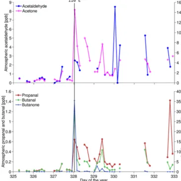
Over the entire cruise track, average atmospheric mixing ratios (10 m a.s.l.) for acetaldehyde, acetone, propanal, butanal and butanone were 0.86, 2.1, 0.15, 0.06 and 0.06 ppb, respectively (Table 1, Fig. 4). The values of acetaldehyde and butanone were on average double the values found in previous studies (compare Table 1 and 3). Acetone and propanal

Figure 4.OVOC concentrations in the air plotted against the day of the year (DOY). Please note that the measurements of the atmospheric data started 3 days later (on day 325) than the water measurements. Vertical line indicates the location of 116^◦E.

were even 1 order of magnitude higher than literature values. Similar elevated atmospheric acetaldehyde mixing ratios were measured on the west coast of Ireland (Mace Head Observatory). Wisthaler et al. (2002) measured similar levels for acetaldehyde and acetone in the continental air masses they encountered above the Indian Ocean. In comparison to most studies listed in Table 3, the coastal region of Borneo seems to be a regional hot spot for atmospheric OVOCs, which might originate from anthropogenic activities, from terrestrial vegetation, and/or due to gas exchange between the ocean and atmosphere.

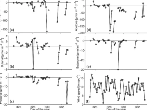
The average computed fluxes over the entire cruise track were negative (into the ocean) for all compounds, except for butanal (Table 1). However, the small magnitude of the fluxes illustrates that the ocean and atmosphere appeared to be near equilibrium for all compounds (Fig. 5). The fluxes into the ocean were mainly caused by localized, strong sinks such as observed in the Balabac Strait (Fig 5a–e; DOY 328) and the open ocean of the Sulu Sea (DOY > 330). In contrast, along the Borneo coast, the ocean was mainly a source of all OVOCs, except for acetaldehyde (Fig. 5; DOY 325–328).

Observations in the open Atlantic and Pacific Ocean found acetaldehyde and propanal fluxes out of the ocean, in contrast to our findings (Tables 1 and 3; Yang et al.,2014a; Zhou and Mopper, 1993; Singh et al., 2003). For acetone, our results are in agreement with previous studies showing that acetone is transported from the atmosphere into the ocean (Table 3).

(10)

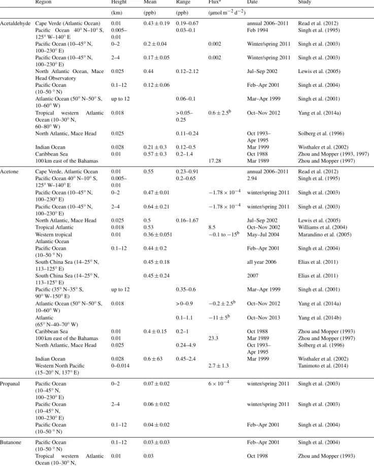
Table 3.Literature values of OVOC concentrations in the atmosphere and their air–sea gas exchange.

Region Height Mean Range Flux^a Date Study

(km) (ppb) (ppb) (µmol m⁻²d⁻²)

Acetaldehyde Cape Verde (Atlantic Ocean) 0.01 0.43±0.19 0.19–0.67 annual 2006–2011 Read et al. (2012) Pacific Ocean 40^◦N–10^◦S,

125^◦W–140^◦E

0.005–

0.01

0.03–0.1 Feb 1994 Singh et al. (1995)

Pacific Ocean (10–45^◦N, 100–230^◦E)

0–2 0.2±0.04 0.002 Winter/spring 2011 Singh et al. (2003)

Pacific Ocean (10–45^◦N, 100–230^◦E)

2–4 0.17±0.05 0.002 Winter/spring 2011 Singh et al. (2003)

North Atlantic Ocean, Mace Head Observatory

0.025 0.44 0.12–2.12 Jul–Sep 2002 Lewis et al. (2005)

Pacific Ocean (10–50^◦N)

0.1–12 0.12±0.06 Feb–Apr 2001 Singh et al. (2004)

Atlantic Ocean (50^◦N–50^◦S, 10–60^◦W)

up to 12 0.06–0.1 Mar–Apr 1999 Singh et al. (2001)

Tropical western Atlantic Ocean (10–30^◦N,

60–80^◦W)

0.018 > 0.05–

0.25

0.6±2.5^b Oct–Nov 2012 Yang et al. (2014a)

North Atlantic, Mace Head 0.025 0.11–0.24 Oct 1993–

Apr 1995

Solberg et al. (1996)

Indian Ocean 0.028 0.21±0.3 0.12–0.5 Mar 1999 Wisthaler et al. (2002)

Caribbean Sea 0.01 0.57±0.3 0.2–1.4 Oct 1988 Zhou and Mopper (1993, 1997)

100 km east of the Bahamas 17.28 Mar 1989 Zhou and Mopper (1997)

Acetone Cape Verde, Atlantic Ocean 0.01 0.55 0.23–0.91 annual 2006–2011 Read et al. (2012) Pacific Ocean 40^◦N–10^◦S,

125^◦W–140^◦E

0.005–

0.01

0.2–0.65 2.94 Singh et al. (1995)

Pacific Ocean (10–45^◦N, 100–230^◦E)

0–2 0.47±0.01 −1.78×10⁻⁴ winter/spring 2011 Singh et al. (2003) Pacific Ocean (10–45^◦N,

100–230^◦E)

2–4 0.64±0.21 −1.78×10⁻⁴ winter/spring 2011 Singh et al. (2003)

North Atlantic, Mace Head 0.025 0.5 0.16–1.67 Jul–Sep 2002 Lewis et al. (2005)

Tropical Atlantic 0.018 0.53 8.5 Oct–Nov 2002 Williams et al. (2004)

Western tropical Atlantic Ocean

0.01 0.36±0.051 −0.1 to−15^b May–Jul 2004 Marandino et al. (2005) Pacific Ocean

(10–50^◦N)

South China Sea (14–25^◦N, 113–125^◦E)

0.45±0.18 all year 2006 Elias et al. (2011)

South China Sea (14–25^◦N, 113–125^◦E)

0.45±0.24 2007 Elias et al. (2011)

Pacific (35^◦N–35^◦S, 90^◦W–150^◦E)

up to 12 0.35–0.6 Mar–Apr 1999 Singh et al. (2001)

Atlantic Ocean (50^◦N–50^◦S, 10–60^◦W)

0.018 > 0–0.9 −0.2±2.5^b Oct–Nov 2012 Yang et al. (2014a) Atlantic

(65^◦N–40–70^◦W)

0.1–1.1 −11±5^b Oct–Nov 2013 Yang et al. (2014b)

Caribbean Sea 0.01 0.4±0.15 0.2–1 Oct 1988 Zhou and Mopper (1993)

100 km east of the Bahamas 0.01 23.3 Mar 1989 Zhou and Mopper (1997)

North Atlantic, Mace Head 0.025 0.24–4.9 Oct 1993–

Apr 1995

Solberg et al. (1996)

Indian Ocean 0.028 0.6±63 0.45–2.4 Mar 1999 Wisthaler et al. (2002)

Western North Pacific (15–20^◦N, 137^◦E)

0–0.014 2.7±1.3 Tanimoto et al. (2014)

Propanal Pacific Ocean (10–45^◦N, 100–230^◦E)

0–2 0.07±0.02 6×10⁻⁴ winter/spring 2011 Singh et al. (2003)

Pacific Ocean (10–45^◦N, 100–230^◦E)

2–4 0.06±0.02 winter/spring 2011 Singh et al. (2003)

Pacific Ocean (10–50^◦N)

Butanone Pacific Ocean (10–50^◦N)

Tropical western Atlantic Ocean (10–30^◦N,

60–80^◦W)

0.01 0.03 Oct 1998 Zhou and Mopper (1993)

aNegative values refer to a flux from the atmosphere into the ocean; positive values indicate fluxes out of the ocean.^bDirect flux was measured using eddy covariance.

(11)

Figure 5.Calculated fluxes of the OVOCs(a–e). Fluxes above the zero line indicate fluxes out of the ocean; fluxes below the zero line indicate fluxes into the ocean. Panel(f)shows the wind speed plotted against the day of the year (DOY).

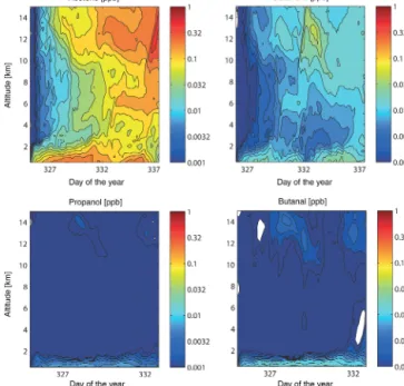
Figure 6.Modeled(a, c)and observed(b, d)atmospheric mixing ratios of butanal(a, b)and propanal(c, d)at the location of the respective measurement. Model simulations have been carried out for all locations where the flux was from the ocean into the atmosphere (also marked by a black edge around the symbols). Modeled mixing ratios were averaged over all data points(a, c)indicated by the number in parts per billion. Observed mixing ratios were averaged separately east and west of 116^◦E (b,d, two black circles). Atmospheric lifetimes (τ )are given in(a)and(c).

To the best of our knowledge, no fluxes were ever reported for butanal and butanone.

The computed fluxes from ocean to atmosphere around the Borneo coast were unexpected, due to the close prox- imity of the cruise track to the coast, the known continen- tally based sources to the atmosphere and the high values of

atmospheric OVOCs that we measured. These fluxes from ocean to atmosphere imply that the production of OVOCs in the ocean around the Borneo coast must be large in order to overcome the high atmospheric mixing ratios observed there. Therefore, this region is a potentially important local source of OVOCs to the atmosphere. It is of interest to know

(12)

whether the calculated ocean–atmosphere fluxes are enough to explain the observed atmospheric OVOC mixing ratios measured along the cruise track or whether these must result from other sources. In addition, we investigated the transport of OVOCs from ocean emissions to the UT, where they can influence HO_xformation.

3.2.1 Horizontal OVOC transport

For all measurement locations with a positive flux (between 12 and 22 stations dependent on OVOC compound), reflecting the ocean being a source of atmospheric OVOCs, we used FLEXPART simulations (see Sect. 2.8) to derive the OVOC mixing ratios within the MBL. We started trajectories con- tinuously over the whole lifetime of the respective gas and loaded them with the amount of OVOCs prescribed by the observed emissions at this location. Based on the FLEX- PART simulations, we derived the mean OVOC mixing ratios from all air parcels released from one measurement location. Given the low density of existing measurements over the area of interest, we did not take into account mixing with air parcels impacted by other (unknown) source regions. This assumption is relatively realistic for the shorter-lived OVOCs with lifetimes of a few hours (butanal and propanal) but less realistic for OVOCs with longer lifetimes of days to weeks (butanone and acetone). For the latter, transport and mixing will have a noticeable impact on the actual mixing ratios. Ig- noring the transport and mixing processes, as done by our method, is equivalent to the assumption that emissions are constant over time (lifetime of the respective OVOC) and space (region specified by transport timescales equivalent to the respective lifetime). Under these assumptions our method offers a useful concept to estimate the maximum atmospheric mixing ratios that could result from the observed oceanic sources.

Figure 6 shows the simulated (a, c) and observed (b, d) mixing ratios of butanal (a, b) and propanal (c, d) depicted at the position of the corresponding measurements. All positions where the flux was from the ocean into the atmosphere are marked by a black edge around the symbol. FLEXPART mixing ratios for butanal based on the observed sea-to-air fluxes were on average 0.033 ppb with maximum values of 0.11 ppb. These values agree very well with the observed mixing ratios of butanal west of 116^◦E, with a mean of 0.039 ppb and a maximum value of 0.16 ppb. However, east of 116^◦E, the observed butanal mixing ratios were on average 0.21 ppb and were thus more than 6 times larger than what could be explained by the local ocean sources. In par- ticular, observed maximum values of up to 1.2 ppb must be driven by other nearby sources. For propanal, positive fluxes occur along the coast off Borneo in the South China Sea but not at the northern tip of Borneo, with one exception around 120^◦E. Atmospheric mixing ratios based on these fluxes are around 0.017 ppb, which is smaller than the mixing ratios observed west of 116^◦E with a mean of 0.037 ppb.

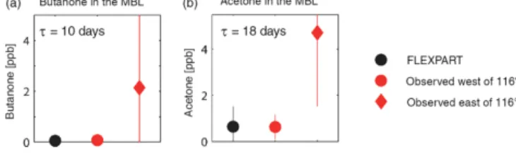
Figure 7.Mean modeled (averaged over all data points, black dot) and observed (averaged east (red dot) and west (red diamond) of 116^◦E) atmospheric mixing ratios of butanone(a)and acetone(b) are shown. The atmospheric lifetimes (τ )are given in the panels.

One can conclude that the local oceanic sources can on average explain about half of the observed mixing ratios in this region. East of 116^◦E, however, the observations are again much larger (0.36 ppb) and cannot be explained at all by local oceanic sources.

Butanone and acetone have longer lifetimes, and released air parcels will spread over a larger area within the respective lifetimes. Thus, we do not show the simulated mixing ratios at the position of the measurements as was done for butanal and propanal, but instead we compared the mean mixing ratios from observations and model simulations (Fig. 7).

The observed atmospheric mixing ratios were split into two regimes west and east of 116^◦E, with relatively low values to the west and higher values to the east for both compounds.

Also for these two longer-lived OVOCs, the observed atmospheric mixing ratios west of 116^◦E were very similar to the maximum amount that can be derived from the observed oceanic sources (Fig. 7). For butanone, observation of 0.07 ppb agreed very well with model results of 0.06 ppb.

The acetone mixing ratios were much higher, again with very good agreement between the model results (0.65 ppb) and observations (0.55 ppb). East of 116^◦E, however, the observed mixing ratios were again much larger (2.1 ppb for butanone and 4.4 ppb for acetone) than what could be explained by oceanic sources, consistent with what has been found for the shorter-lived OVOCs.

Overall, the observed atmospheric OVOCs can be split into two regimes, where one can be explained by the local oceanic sources (west of 116^◦E) and the other requires additional terrestrial, anthropogenic or marine sources (east of 116^◦E). Analyzing the variability in atmospheric OVOCs along the cruise track, we found significant correlations between acetone and butanal (rs=0.91,pvalue 0.001) as well as between acetone and propanal (r_s=0.85,pvalue 0.001).

Much of this variability is due to the presence of areas east of 116^◦E, with large sources reflected in the measurements of all three OVOCs (Fig. 4), suggesting that the same drivers (e.g., anthropogenic sources) control the occurrence of these hotspots.

To further explore the higher mixing ratios observed east of 116^◦E, we focused on the shorter-lived OVOCs, butanal and propanal, using the backward trajectory calculations over

(13)

Figure 8.Backward trajectories over 24 h from all OVOC measurement locations are shown. The trajectories are color-coded according to the atmospheric transport regime.

1 day. The backward trajectories (Fig. 8) display air mass transport from east to west over the 24 h preceding each measurement. Note that FLEXPART trajectories west of Borneo (south of 4^◦N, not shown here) agree well with HYSPLIT trajectories used for an airborne tracer experiment conducted during the SHIVA campaign (Ren et al., 2015). For better visibility, we split the trajectories into five different groups according to slightly different transport patterns. Groups 1, 2 and 3 (green, light blue and magenta trajectories), encom- passing most air masses observed east of 116^◦E, crossed the coastline of the Philippines within this time period. Most air masses west of 116^◦E (red and blue trajectories), however, were too far from the Philippine coast to have experienced terrestrial or anthropogenic influence in the 24 h before these samples were taken onboard of the ship. The inability of the local oceanic sources to explain the high atmospheric mixing ratios east of 116^◦E strongly suggests additional terrestrial or anthropogenic sources. The backward trajectory analysis further supports this hypothesis. It is also possible that localized marine strong source areas exist at some short distance from the cruise track area. However, we think this is less likely as these hotspots would need to be much larger than anything measured during the cruise to explain atmospheric mixing ratios 10 to 20 times larger than the ones resulting from the observed oceanic sources.

3.2.2 Implications of oceanic sources on the UT

To assess the potential importance of the local OVOC source of upper-tropospheric HO_x formation in the convective region of the Pacific, we computed the vertical transport using FLEXPART for acetone, butanone, propanal and butanal (Fig. 9). Acetaldehyde was left out of this analysis because there were only two data points with fluxes out of the sea surface to the atmosphere. The vertical trajectory mixing ratios were calculated by emitting the average value of the computed sea-to-air fluxes over 1 month in the source location and prescribing tropospheric lifetimes for the loss term (see

Figure 9.Vertical distribution of the OVOCs derived from FLEX- PART model simulations. OVOCs are released from the measurement locations over the time period of the cruise according to the respective ocean–atmosphere flux.

Sect. 2.8 and 2.9). For the aldehydes, the highest mixing ratios were computed for the lower troposphere, with values up to approximately 0.01 ppb. Values aloft, up to approximately 15 km, did not exceed 0.003 ppb for both propanal and butanal. The ketone vertical profiles showed maxima in both the lower 2 km and above 10 km, with values exceeding 0.30 ppb for acetone and 0.10 ppb for butanone. This is likely due to the longer tropospheric lifetimes of the ketones than the aldehydes, as the computed ketone sources to the atmosphere were not always larger than the aldehydes (Fig. 5).

It was previously thought that low levels of water vapor in the UT prevent HO_xformation there. In the 1990s, it became clear that this idea was not valid (Singh et al., 1995; Chat- field and Crutzen, 1984; Prather and Jacob, 1997). Wennberg et al. (1998) sought to understand observed levels of OH in the troposphere by using both the O(1D)+H2O reaction, as well as acetone photolysis (using approximately 0.30 ppb of acetone). They found that at heights between 9 and 14 km, the inclusion of acetone photolysis improved the model measurement agreement. At heights from 14 to 16 km, the inclusion of acetone photolysis resulted in near perfect agreement between model and measurement, suggesting acetone as the main source of OH at these heights. However, Blitz et al. (2004) revised the acetone quantum yield downward, resulting in less acetone loss, which would also result in lower values of computed OH. It is likely that other OVOCs with similar photochemical properties, such as butanone, are also present in the UT and could compensate for this downward revision. Here we calculated that a combined value

(14)

greater than 0.4 ppb of acetone and butanone from a spa- tially limited ocean source region in the South China Sea can be present in the UT (Fig. 9). Data recently obtained from the CARIBIC campaign showed that acetone values between 0.30 and 1.2 ppb are in fact observed in the UT (Neumaier et al., 2014). By combining their data with simulations from the global chemistry–climate modeling system (ECHAM/MESSy Atmospheric Chemistry, EMAC), Neu- maier et al. (2014) showed that UT HO_x production from acetone is significant all year round, reaching an average of 60 % of that from ozone photolysis in summer and 95 % in fall. It should be noted that CARIBIC took place in the mid- latitudes, not in the tropics like SHIVA, but their reported HOx precursors were similar to SHIVA (water vapor range:

CARIBIC 20–140 ppm, SHIVA 0–40 ppm; ozone: CARIBIC 50–150 ppb, SHIVA 20–100 ppb (data not shown)). Thus, ketones in the UT from ocean sources in the western Pacific Ocean have the potential to contribute at least 30 % of UT mixing ratios, having an important influence on HO_xforma- tion there. In addition, using sensitivity studies with EMAC, Neumaier et al. (2014) found that one of the major uncer- tainties in quantifying UT HO_x formation from acetone is the acetone mixing ratio distribution. Therefore, more observations and forward trajectory calculations from the atmospheric boundary layer are needed to understand the important role of acetone and other longer-lived OVOCs in the distribution of HO_xin the UT.

4 Summary

For the first time, a suite of OVOCs were measured simultaneously in the surface water and overlying atmosphere in the South China Sea and Sulu Sea. Sea surface concentrations of acetone, propanal, butanal and butanone correlated with each other, indicating similar sources and sinks in the surface water. Phytoplankton seemed to be the main source of acetone, propanal and butanal in the South China and Sulu seas. Ac- etaldehyde and butanone seemed to be produced by both phytoplankton and terrestrial and marine-derived FDOM components.

The South China Sea seemed to be a regional hot spot for atmospheric OVOCs and the air–sea gas exchange was on average into the ocean, thus, atmospheric OVOCs seemed to be an additional important source (up to 44 %) for OVOCs in the surface ocean. However, local fluxes from the ocean into the atmosphere along the coast off Borneo, implied that local coastal marine sources can be sufficient to drive fluxes from ocean to atmosphere, even when atmospheric mixing ratios were large. West of 116^◦E the flux of marine OVOCs into the atmosphere could explain the atmospheric mixing ratios of OVOCs, while east of 116^◦E terrestrial and anthropogenic sources were responsible for the elevated atmospheric OVOCs. The longer-lived marine-derived ketones, acetone and butanone, were calculated to contribute more

than 0.4 ppb to the UT in this convective region and may be important for HO_xformation above the South China Sea.

Data availability. All data (seawater and atmospheric OVOC data, OVOC flux data, nitrate, salinity and FDOM) can be retrieved from the Supplement and will be available in the PANGAEA database.

Phytoplankton data are already available at the PANGAEA database (https://doi.org/10.1594/PANGAEA.848589; Bracher, 2014).

The Supplement related to this article is available online at https://doi.org/10.5194/acp-17-10837-2017- supplement.

Author contributions. CS and CM designed the experiments and measured the samples of OVOCs and FDOM. CS performed sta- tistical calculations, wrote most of the Sects. 1–3.2 (first paragraph and summary), and created Figs. 2–5, S1 and Table S1. CM wrote Sect. 3.2 and 3.2.2. ST performed the FLEXPART model analysis, wrote Sects. 2.8 and 3.2.1, and created Figs. 6–9. SL performed the FDOM PARAFAC calculations and wrote Sect. 2.5. WC took phytoplankton samples, measured them, performed the CHEMTAX analysis and wrote Sect. 2.3 together with AB. AB created Fig. 1.

BQ wrote Sect. 2.1. All authors contributed to reviewing and im- proving the text.

Competing interests. The authors declare that they have no conflict of interest.

Acknowledgements. Thanks go to the captain and crew of the R/V Sonne. We thank Sonja Wiegmann, Mariana Soppa and Joseph Palermo for supporting the phytoplankton sampling during the cruise and Sonja Wiegmann for the HPLC pigment analysis. We gratefully acknowledge the NASA Goddard Space Flight Center, Ocean Biology Processing Group, for providing SeaWiFS Ocean Color Data CDOM. We thank Francois Steinmetz (HYGEOS) for supplying Polymer-MERIS Chl data (also for campaign planning) and ESA for MERIS level-1 satellite data. This work was supported by the EU project SHIVA under grant agreement no. FP7-ENV- 2007-1-226224 and by the BMBF grants SHIVA-Sonne (FKZ:

03G0218A). We gratefully acknowledge the “Studienstiftung des Deutschen Volkes” for providing the “Promotionsstipendium” for Cathleen Schlundt to conduct this research study. Astrid Bracher and Wee Cheah were funded via the HGF Young Investigator Group PHYTOOPTICS (VH-NG-300) from the Helmholtz Asso- ciation through the President. Astrid Bracher’s contribution was also partly funded by ESRIN/ESA within the SEOM (Scientific Exploration of operational missions) – Sentinel for Science Synergy (SY-4Sci Synergy) program via the project SynSenPFT.

Additional funding for Cathleen Schlundt, Christa A. Marandino and Sinikka T. Lennartz came from the Helmholtz Young Investi- gator Group of Christa A. Marandino, TRASE-EC (VH-NG-819), from the Helmholtz Association through the President’s Initiative and Networking Fund and the GEOMAR Helmholtz-Zentrum für Ozeanforschung Kiel. We gratefully thank Mingxi Yang and