Progress in Oceanography 189 (2020) 102446
Available online 30 September 2020
0079-6611/© 2020 The Author(s). Published by Elsevier Ltd. This is an open access article under the CC BY license (http://creativecommons.org/licenses/by/4.0/).
Abyssal food-web model indicates faunal carbon flow recovery and
impaired microbial loop 26 years after a sediment disturbance experiment
Dani ¨ elle S.W. de Jonge
a,b,1,2, Tanja Stratmann
b,c,d,*,1, Lidia Lins
e, Ann Vanreusel
e, Autun Purser
f, Yann Marcon
g, Clara F. Rodrigues
h, Ascens ˜ ao Ravara
h, Patricia Esquete
h, Marina R. Cunha
h, Erik Simon-Lled ´ o
i, Peter van Breugel
b, Andrew K. Sweetman
j,
Karline Soetaert
b, Dick van Oevelen
baFaculty of Mathematics and Natural Sciences, University of Groningen, P.O. Box 11103, 9700 CC Groningen, the Netherlands
bNIOZ Royal Netherlands Institute for Sea Research, Department of Estuarine and Delta Systems, and Utrecht University, P.O. Box 140, 4400 AC Yerseke, the Netherlands
cDepartment of Earth Sciences, Utrecht University, Vening Meineszgebouw A, Princetonlaan 8a, 3584 CB Utrecht, the Netherlands
dHGF MPG Joint Research Group for Deep-Sea Ecology and Technology, Max Planck Institute for Marine Microbiology, Celsiusstr. 1, 28359 Bremen, Germany
eMarine Biology Research Group, Ghent University, Krijgslaan 281 S8, 9000 Ghent, Belgium
fHGF MPG Joint Research Group for Deep-Sea Ecology and Technology, Alfred Wegener Institute, Am Handelshafen 12, 27570 Bremerhaven, Germany
gMARUM – Center for Marine Environmental Sciences, General Geology – Marine Geology, University of Bremen, 28359 Bremen, Germany
hDepartamento de Biologia & Centro de Estudos do Ambiente e do Mar (CESAM), Departamento de Biologia, Universidade de Aveiro, Campus de Santiago, 3810-193 Aveiro, Portugal
iNational Oceanography Centre, University of Southampton Waterfront Campus, European Way, Southampton SO14 3ZH, UK
jDeep-Sea Ecology and Biogeochemistry Research Group, The Lyell Centre for Earth and Marine Science and Technology, Heriot-Watt University, Edinburgh EH14 4AS, UK
A R T I C L E I N F O Regional index terms:
South-East Pacific Peru Basin
DISCOL Experimental Area Keywords:
Ecosystem disturbance Deep-seabed mining Abyssal plains Ferromanganese nodules Linear inverse model
A B S T R A C T
Due to the predicted future demand for critical metals, abyssal plains covered with polymetallic nodules are currently being prospected for deep-seabed mining. Deep-seabed mining will lead to significant sediment disturbance over large spatial scales and for extended periods of time. The environmental impact of a small-scale sediment disturbance was studied during the ‘DISturbance and reCOLonization’ (DISCOL) experiment in the Peru Basin in 1989 when 10.8 km2 of seafloor were ploughed with a plough harrow. Here, we present a detailed description of carbon-based food-web models constructed from various datasets collected in 2015, 26 years after the experiment. Detailed observations of the benthic food web were made at three distinct sites: inside 26-year old plough tracks (IPT, subjected to direct impact from ploughing), outside the plough tracks (OPT, exposed to settling of resuspended sediment), and at reference sites (REF, no impact). The observations were used to develop highly-resolved food-web models for each site that quantified the carbon (C) fluxes between biotic (ranging from prokaryotes to various functional groups in meio-, macro-, and megafauna) and abiotic (e.g. detritus) com- partments. The model outputs were used to estimate total system throughput, i.e., the sum of all C flows in the food web (the ‘ecological size’ of the system), and microbial loop functioning, i.e., the C-cycling through the prokaryotic compartment for each site. Both the estimated total system throughput and the microbial loop cycling were significantly reduced (by 16% and 35%, respectively) inside the plough tracks compared to the other two sites. Site differences in modelled faunal respiration varied among the different faunal compartments.
Overall, modelled faunal respiration appeared to have recovered to, or exceeded reference values after 26-years.
The model results indicate that food-web functioning, and especially the microbial loop, have not recovered from the disturbance that was inflicted on the abyssal site 26 years ago.
* Corresponding author.
E-mail address: t.stratmann@uu.nl (T. Stratmann).
1 These authors have contributed equally to this work.
2 Current address: The Lyell Centre for Earth and Marine Science and Technology, Heriot-Watt University, Edinburgh, Scotland EH12 4AS, UK.
Contents lists available at ScienceDirect
Progress in Oceanography
journal homepage: www.elsevier.com/locate/pocean
https://doi.org/10.1016/j.pocean.2020.102446
Received 3 April 2020; Received in revised form 21 September 2020; Accepted 22 September 2020
1. Introduction
The future demand for metals such as nickel, copper, and cobalt may cause supply shortages from terrestrial mines, thus creating the perceived need to mine these mineral resources elsewhere (Hein et al., 2013). Marine mineral deposits with high metal concentrations, such as polymetallic nodules, polymetallic sulphides, and cobalt-rich ferro- manganese crusts, are therefore being prospected, but extraction of these substrates from the seafloor will result in significant environ- mental impacts. These impacts will include removal of hard substrate, habitat modification and destruction (Oebius et al., 2001), the release of toxic metals (Koschinsky et al., 2003), creation of sediment plumes (Oebius et al., 2001; Murphy et al., 2016), and noise and light pollution (Miller et al., 2018).
To investigate how to achieve the minimum possible effects of mining on deep-sea biota, scientists have performed a variety of ex- periments, mimicking small-scale disturbances and recording their ef- fects. Previous sediment disturbance experiments to study the response of the deep-sea ecosystem were mainly focused on specific faunal groups (Bluhm, 2001; Ingole et al., 2001, 2005a, 2005b; Miljutin et al., 2011;
Rodrigues et al., 2001; Vanreusel et al., 2016). In general, varying de- grees of recovery were recorded, with no recovery back to control or baseline conditions for almost all faunal groups over decadal time-scales (Jones et al., 2017). Generally, large sessile species have either not recovered at all or at best, recovered slower than small mobile species (Gollner et al., 2017; Jones et al., 2017) (e.g. large suspension feeders;
Simon-Lled´o et al., 2019b). Interest in the impact of sediment distur- bance on abyssal sediment biogeochemistry has increased relatively recently (Haffert et al., 2020; Paul et al., 2018; Volz et al., 2020).
The most comprehensive of these disturbance studies is the
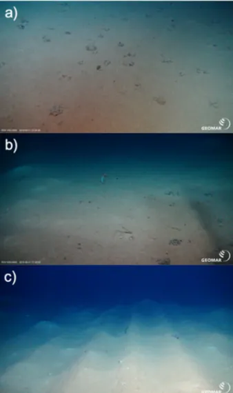
‘DISturbance and reCOLonization’ (DISCOL) experiment, which was performed in 1989, during which a manganese nodule area of 10.8 km2 was ploughed diametrically 78 times with an 8 m-wide plough-harrow, thereby creating plough tracks with nodules mixed into the top 10–20 cm of sediment (Thiel et al., 1989). Next to these plough tracks, the seafloor was not directly disturbed, but the sediment and nodules were covered with a layer of resuspended sediments. Food-web recovery was monitored during five follow-up cruises between March 1989 and September 2015 (Thiel et al., 1989; Schriever, 1990; Schriever and Thiel, 1992; Schriever et al., 1996; Boetius, 2015; Greinert, 2015). In summary, 26 years after the DISCOL experiment the tracks with reset- tled sediment could still be clearly observed (Gausepohl et al., 2020) (Fig. 1) and the different disturbance levels hosted a distinct megafauna community (Simon-Lled´o et al., 2019b). Although deposit-feeder den- sities, including holothurians, were overall not substantially different among sites after 26 years (Simon-Lled´o et al., 2019b; Stratmann et al., 2018c), macrofauna and megafauna densities, especially suspension feeders, were significantly depressed inside the plough track compared to outside the plough tracks and reference sites (Drazen et al., 2019;
Simon-Lled´o et al., 2019b; Stratmann et al., 2018a). In addition, 26 years after the initial ploughing and mixing of the upper-sediment layer, porewater chemistry in sediments from the DISCOL experimental area (DEA) had recovered, but distinct differences in metal distributions between disturbed and undisturbed sediments still existed (Paul et al., 2018) and microbial mediated biogeochemical functions were still impaired (Vonnahme et al., 2020). Modelling results indicated that removal of the upper sediment layer might result in even slower re- covery rates of geochemical sediment processes compared to the re- covery process observed when sediments were mixed (Haffert et al., 2020).
So far, the DISCOL follow-up studies focussed on temporal dynamics.
However, because not all ecosystem components were addressed during the early years of the experiment, i.e., prokaryotes, meiofauna, and high taxonomic resolution of megafauna were missing, an integrated food- web perspective is lacking in these time-series analyses. During an extensive sampling campaign at the DISCOL site in 2015, data on many
ecosystem components, including the smaller metazoan (e.g. nema- todes) and microbial domain, were collected. This recent dataset allows the construction of food-web models at spatially separated disturbed and reference sites. Comparing ecosystem functioning at sediments disturbed 26 years ago to sediments at nearby reference sites can help to understand temporal recovery dynamics on decadal time scales.
Food-web models describe the trophic interactions within an ecological community and provide an integrative approach to study ecosystem-wide effects of perturbations, like the DISCOL sediment disturbance (Allesina and Pascual, 2008). The quantification of trophic interactions in a marine network is, however, often hampered by the difficulty of data collection, especially in remote areas like the open or deep ocean. Different methods like top-down mass-balancing (e.g. Hunt et al., 1987) and inverse modelling (Christensen and Pauly, 1992; van Oevelen et al., 2010) have been devised to estimate the fluxes within a food web. Resolved food webs can reveal emergent properties of ecosystem functioning, which can be captured by network indices (Latham, 2006; Heymans et al., 2014).
Network indices can summarize the characteristics of the complex ecological networks at the disturbed and reference sites into single values, which can then be compared among the different disturbance levels. The topological size and complexity can be captured by the number of links (L), linkage density (LD), i.e., the average number of
Fig. 1. Representative pictures of the sediments at (a) reference sites, (b) outside plough tracks, and (c) inside plough tracks taken during the Sonne SO242-2 cruise to the DISCOL site in 2015. Photos by ROV Kiel 6000 (GEO- MAR, Kiel, Germany).
links per compartments, and connectance (C), i.e., the proportion of realised links (Gardner and Ashby, 1970). Trophic level (TL) signifies the position of a trophic compartment in the food chain and is related to resource availability and transfer efficiency (Post, 2002). In addition, C cycling is represented by total system throughput (T..), i.e. the sum of all C flows in the food web, reflecting the ‘ecological’ size of the system (Latham, 2006), and by the Finn’s Cycling Index (FCI), i.e. the propor- tion of C cycling due to recycling processes, reflecting structural dif- ferences and the efficiency of C usage in a system (Finn, 1976). Network indices are robust to a fair extent of variation in input data and network structure (Kones et al., 2009; Heymans et al., 2014). This underlines their suitability for analysing models that cannot be fully parameterized with empirical data, like the food-web model from the remote DISCOL experimental area where direct measurements are limited.
Here, we integrate a recent dataset collected from the DISCOL experiment in 2015 to develop highly resolved food webs of the following sites: inside plough tracks (IPT), outside plough tracks (OPT), i.e., right next to the plough tracks, and reference sites (REF), i.e., an
area 4 km from the DEA assumed unaffected by the disturbance. Linear inverse modelling was used to estimate C flows among food-web com- partments in pre-defined topological food webs based on information comprising biomass, feeding preferences, growth efficiencies, and respiration rates (V´ezina and Platt, 1988; van Oevelen et al., 2010). The resolved linear inverse models for the different disturbance levels allowed us to obtain estimates of C flows that could not be measured in situ and determine ecosystem-wide recovery after a small-scale benthic disturbance on decadal timescales. Specifically, system characteristics that we would expect to see at an impacted site are (1) reduced ecosystem complexity due to species mortality reflected by reduced LD and C indices, (2) reduced mean and maximum TL due to reduced resource availability, impaired metabolic efficiency, and reduction of top predators, (3) reduced productivity of different trophic groups re- flected by impaired respiration, and (4) reduced C cycling and recycling efficiency reflected by a reduced T.. and FCI respectively, with a specific focus on C cycling in the microbial loop and the scavenging pathway.
Results were compared to other abyssal plain food-web models and
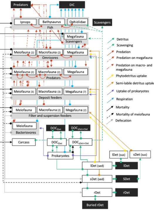
Fig. 2.Schematic representation of the topolog- ical food web used for the linear inverse models.
White boxes show all food-web compartments inside the model, whereas black boxes show external compartments that were not explicitly modelled. Grey boxes show the feeding types bacterivores, filter and suspension feeders, de- posit feeders, predators, omnivores, and fish. The white boxes enclosed by the grey boxes represent the size classes meiofauna, macrofauna, mega- fauna, and the specific fish taxa Ipnops sp., Bath- ysaurus mollis, and Ophidiidae. The numbers in brackets behind the size classes specify the number of food-web compartments of that spe- cific size class and feeding type. The arrows represent C flows leading from the C source (arrow ending with a big dot) to C sink (arrow- head). Abbreviations are: DOC = dissolved organic matter, lDet (sus) = suspended labile detritus, sDet (sus) = suspended semi-labile detritus, lDet (sed) =labile detritus in the sedi- ment, sDet (sed) = semi-labile detritus in the sediments, rDet =refractory detritus.
interpreted with an outlook on deep-seabed mining.
2. Materials & methods
2.1. Study site
The Peru Basin in the south-east Pacific extends from the East Pacific Rise at 110◦W to the Atacama Trench west of the coast of Peru (Klein, 1993; Bharatdwaj, 2006). In the North, the Peru Basin borders on the Carnegie Ridge at 5◦S and in the South, it borders on the Sala-y-Gomez Ridge and the Nazca Ridge at 24◦S (Klein, 1993; Bharatdwaj, 2006). The Peru Basin has a water depth ranging between 3,800 and 4,400 m (Wiedicke and Weber, 1996; Greinert, 2015) and a bottom water tem- perature of 2.9 ◦C (Boetius, 2015). The DEA is located in the northern part of the Peru Basin at 07◦04.4′S, 88◦27.6′W (Thiel et al., 1989). In 2015, the long-term impacts of the original disturbance (1989) were assessed by taking measurements inside plough tracks, outside plough tracks, i.e., areas next to plough-tracks where re-suspended sediment settled, and at reference sites 4 km away from the DEA that were considered to be unaffected by the disturbance (Fig. 1).
2.2. Food-web structure
Faunal compartments in the food web were defined using size-classes (meiofauna MEI, macrofauna MAC, and megafauna MEG) and feeding types (bacterivores B, filter- and suspension feeders FSF, epistrate feeders EF, non-selective deposit-feeders NSDF, sub-surface deposit feeders SSDF, surface deposit feeders SDF, omnivores OF, predators P, scavengers S).
Metazoan meiofauna (>32 µm) consisted of Nematoda, Harpacti- coida and their nauplii, Polychaeta, Ostracoda, Tardigrada, Bivalvia, Kinorhyncha, Gastrotricha, Tanaidacea, Cyclopoida, Gastropoda, Lor- icifera, Oligochaeta, Rotifera, and Isopoda. Based on the four most abundant nematode families in the abyssal CCZ (Miljutin et al., 2011), Nematoda were divided into the feeding types non-selective deposit feeders (NemNSDF), epistrate feeders (NemEF), and omnivores/ pred- ators (NemOP) (Table A1). Meiofauna polychaetes were divided into feeding types following the feeding type classification for macrofauna polychaetes. The remaining metazoan meiofauna were classified as filter and suspension feeders (MeiFSF), bacterivores (MeiB), deposit feeders (MeiDF), predators (MeiP), and omnivore feeders (MeiOF) based on reported feeding ecologies in peer-reviewed literature (Table A1).
Metazoan macrofauna taxa included Polychaeta, Amphipoda, Tanaidacea, Isopoda, Cumacea, Bivalvia, Gastropoda, Scaphopoda, Echinoidea, and Ophiuroidea. The polychaetes were identified to family level, so the review paper by Jumars et al. (2015) was used to classify the polychaetes into suspension feeders (PolSF), surface deposit feeders (PolSDF), subsurface deposit feeders (PolSSDF), predators (PolP), and omnivores (PolOF) (Table A2). For each site, the community composi- tion of polychaete families was used to specify the relative presence of each feeding-type. All other macrofauna taxa were classified as filter and suspension feeders (MacFSF), deposit feeders (MacDF), predators (MacP), and omnivores (MacOF) based on reported feeding ecologies in peer-reviewed literature (Table A2).
Megafauna taxa of the phyla Annelida, Arthropoda, Chordata (except fish), Cnidaria, Echinodermata (except Holothuria), Hemichordata, Mollusca, and Porifera were combined in the feeding types deposit feeders (MegDF), suspension and filter feeders (MegFSF), surface de- posit feeders (MegSDF), subsurface deposit feeders (MegSSDF), preda- tors (MegP), omnivores (MegOF), and scavengers (MegS) (Table A3).
Furthermore, the five holothurian morphotypes Amperima sp., Bentho- dytes typica, Mesothuria sp., Peniagone sp. (including Peniagone sp. mor- photype “palmata”, Peniagone sp.1, Peniagone sp. 2 benthopelagic), and Psychropotes depressa that collectively contributed between 80% (OPT) and 83% (REF) to the total holothurian biomass (Stratmann et al., 2018c) were kept as separate food-web compartments (Table A3). All
other holothurian morphotypes were summed as filter and suspension feeding holothurians (HolFSF) and surface-deposit feeding holothurians (HolSDF) based on their feeding ecology (Table A3).
Fish were divided into Bathysaurus mollis, Ipnops sp., and Ophidiidae.
Bathysaurus mollis predates on Ipnops sp., Ophidiidae, Amphipoda, Cir- ripedia, Isopoda, Munidopsidae, Probeebei sp., Pycnogonida, and other crustaceans, and it also scavenges carrion (Sulak et al., 1985; Crabtree et al., 1991; Drazen and Sutton, 2017). Ipnops sp. predates upon Poly- chaeta, Amphipoda, Isopoda, other crustaceans, and Mollusca (Crabtree et al., 1991; Drazen and Sutton, 2017). Ophidiidae predates on Poly- chaeta, Amphipoda, Isopoda, other crustaceans, Mollusca and it scav- enges carrion (Crabtree et al., 1991; Drazen and Sutton, 2017; Gerringer et al., 2017). The contribution of the different megafaunal compart- ments to the fish diet (Table A4) was calculated based on the contri- bution of each prey taxon to the feeding-type specific C stock.
The non-faunal food-web compartments included prokaryotes (Pro), carrion (CARC), dissolved organic carbon (DOC), and detritus divided into different lability classes, namely labile detritus (lDet), semi-labile detritus (sDet), and refractory detritus (rDet) (sensu van Oevelen et al., 2012).
2.3. Food-web links
Carbon transfer links in the food web were implemented as shown in Fig. 2. Suspended and sedimentary (semi-)labile detritus and sedimen- tary refractory detritus receive C input from an external (semi-)labile detritus and an external refractory detritus pool. Suspended labile and semi-labile detritus were C sources for all filter- and suspension feeders (MeiFSF, MacFSF, PolSF, MegFSF, and HolFF). Nematode epistrate feeders (NemEF) fed on sedimentary labile detritus and prokaryotes.
Sedimentary labile detritus, semi-labile detritus, and prokaryotes were grazed upon by non-selective deposit feeders (NemNSDF), surface de- posit feeders (PolSDF and HolSDF), subsurface deposit feeders (PolSSDF), other deposit feeders (MeiDF, MacDF, and MegDF), deposit- feeding holothurians (Amperima sp., Benthodytes sp., Mesothuria sp., Peniagone sp., and Psychropotes sp.), and omnivores (NemOP, MeiOF, PolOF, MacOF, and MegOF).
Predators and omnivores predated on all faunal organisms from the same and smaller size classes. Meiofauna and macrofauna predators (NemOP, MeiP, PolP, MacP) also predated on their own compartment.
Additionally, omnivores and scavengers (MegS, Bathysaurus mollis, and Ophidiidae) scavenged from the carrion compartment. Ipnops sp. pre- dated upon MegFSF, MegDF, MegP, and MegS (Table A4). Bathysaurus mollis predated upon MegFSF, MegDF, MegP, MegS, Ipnops sp., and Ophidiidae, and Ophidiidae predated upon MegFSF, MegDF, MegP, and MegS (Table A4).
All faunal compartments produced faeces that contributed to the semi-labile and refractory detritus pool. Furthermore, nematode and other metazoan meiofauna mortality contributed to the semi-labile detritus pool, whereas dead polychaetes, other metazoan macrofauna, holothurians, other megafauna, and fishes contributed to the carrion pool. Sedimentary labile, semi-labile, and refractory detritus hydrolysed to DOC, which was taken up by prokaryotes.
Prokaryotes respired C as dissolved inorganic carbon (DIC) and contributed to the DOC pool by virus-induced prokaryotic lysis. The DOC pool further increased by influx of external DOC to the system.
Other C fluxes out of the model included the burial of refractory detritus, respiration by all faunal compartments, the efflux of DOC, external scavengers scavenging carrion, and predation on polychaetes, other macrofauna, holothurians, other megafauna, and fishes by external predators.
For the incorporation of isotope data, several processes (detritus uptake, defecation, and respiration) were specifically divided into labile detritus-derived fluxes and semi-labile and/or refractory detritus- derived fluxes (see ‘Incorporation of isotope tracer data’).
2.4. Data sources
2.4.1. Carbon stocks of food-web compartments
To quantify the labile, semi-labile, and refractory detritus, and pro- karyote pools in the upper 5 cm of sediment of the different study sites, sediment samples were taken with multi corers from inside the cham- bers of benthic landers after lander retrieval, and ROV-deployed push corers and blade corers (Table A5).
The labile detritus pool is defined as the average chlorophyll-a (chl- a) content in the surface sediment (sensu van Oevelen et al., 2011a), and was measured by Vonnahme et al. (2020, IPT corresponded to the mi- crohabitats ‘Furrow’ and ‘Ridge’ combined). Chl-a was extracted in 90%
acetone, measured photometrically following Jeffrey’s and Humphrey (1975) approach for mixed phytoplankton populations and converted to C units using a C to chl-a-ratio of 40 (De Jonge, 1980).
The semi-labile detritus pool is defined as the sum of proteins, car- bohydrates, and lipids, i.e., the so-called biopolymeric carbon (Fabiano et al., 1995). The concentration of total hydrolysable amino acids (THAA) in 0.4 g freeze-dried surface sediment per sample was measured following Maier et al. (2019). As neither lipid nor carbohydrate con- centrations in the sediment were measured, a ratio of 0.12 : 1 : 1.32 for lipids : THAAs : carbohydrates (Laubier and Monniot, 1985) was used to calculate the total biopolymeric carbon pool.
The refractory detritus pool refers to the particulate organic carbon (POC) stock in the surface sediment that was measured by Vonnahme et al. (2020, IPT corresponded to the microhabitats ‘Furrow’ and ‘Ridge’
combined) and from which the labile and semi-labile detritus pools were subtracted.
Prokaryotic abundance in the surface sediment (0–1 cm) was determined by Vonnahme et al. (2020, IPT corresponded to the micro- habitats ‘Furrow’ and ‘Ridge’ combined) using the Acridine Orange Direct Count (AODC) method. Subsequently, we converted prokaryotic abundances into prokaryotic C stock (mmol C m−2) by multiplying the abundance with a factor of 12.5 fg C cell−1, i.e., C content of prokaryotic cells in waters from the southern subtropical Pacific (15◦S) (Fukuda et al., 1998). The 0–1 cm prokaryotic C stock was extrapolated to the 0–5 cm prokaryotic C stock as:
Cstock0−5cm=
∑
Cstock0−1cm×e−0.1×(x+1) (1) based on previous C stock measurements in the Peru Basin (For- schungsverbund Tiefsee-Umweltschutz, unpubl.). Cstock0−1cm corre- sponds to the C stock in the surface sediment (0–1 cm) and (x +1) is the sediment interval (i.e., x =1 for the sediment interval 1–2 cm).
Metazoan meiofaunal C stock was determined from ROV-deployed push corers (7.4 cm inner-diameter) (Table A5) of which the upper 5 cm of sediment was preserved in 4% borax-buffered formaldehyde at room temperature. Ashore, sediment samples were washed over a 32-μm sieve and metazoan meiofauna was extracted by density centrifugation with Ludox HS40 (Dupont) at 3000 rpm. A subset of 100–150 metazoan meiofauna specimens per sample were identified to higher taxonomic level, i.e. to the rank of order, subclass, class, or phyla using Higgins and Thiel (1988), and counted with a stereomicroscope (Leica MZ8, 50× magnification) to determine taxon-specific densities. When the number of metazoan meiofauna individuals was lower than 100, the whole sample was counted. Stocks of all metazoan meiofauna taxa were calculated by multiplying the taxon-specific densities with the conver- sion factors from Table A1. Stocks of the different taxa were grouped according to feeding type as described above (see ‘Food-web structure’).
Metazoan macrofauna were collected with a 50×50×60 cm box- corer at all three sites (Table A5). The sediment of the upper 5 cm was sieved on a 500-μm sieve and all organisms that were retained on this sieve were preserved in 96% un-denaturated ethanol and stored at
− 20 ◦C. Ashore, all macrofauna samples were sorted under stereomi- croscopes (Olympus SZX9, Olympus SZH10, Leica MZ125) and a com- pound microscope (Olympus BX50 MO). They were identified to higher
taxon level, i.e., to the rank of order, subclass, class, or phyla. Macro- fauna polychaetes were identified to family level. For the identifications a vast list of papers was used specialized in the different taxa at major group level as well as at family, genus, and even species level. Macro- fauna and macrofaunal polychaete stocks were calculated by multi- plying the macrofauna and macrofaunal polychaete densities from the box corers with taxon-specific individual biomass data from Table A2.
Table 1
Carbon stocks (mmol C m−2) of the food-web compartments at reference sites (REF), outside plough tracks (OPT), and inside plough tracks (IPT).
Compartment REF OPT IPT
Detritus
Labile detritus (lDet) 6.37 5.70 5.25
Semi-labile detritus (sDet) 406 538 367
Refractory detritus (rDet) 6955 7168 7808
Prokaryotes
Prokaryotes (Pro) 8.52 8.48 8.17
Meiofaunal Nematoda
Non-selective deposit feeding nematodes
(NemNSDF) 0.22 0.42 0.33
Epistrate feeding nematodes (NemEF) 0.11 0.21 0.17 Omnivory/ predatory nematodes
(NemOP) 0.11 0.21 0.17
Metazoan meiofauna (except Nematoda) Meiofauna filter and suspension feeders
(MeiFSF) 3.87 ×
10−2 6.70 ×
10−2 4.34 × 10⁻² Meiofauna bacterivores (MeiBF) 4.66 ×
10−4 8.09 ×
10−4 1.07 × 10⁻³ Meiofauna deposit feeders (MeiDF) 1.33 2.09 1.82 Meiofauna predators (MeiP) 6.61 ×
10−2 6.85 ×
10−2 3.51 × 10⁻²
Meiofauna omnivores (MeiO) 0.18 0.37 0.48
Macrofaunal Polychaeta
Polychaete suspension feeders (PolSF) 0.14 0.21 0.24 Polychaete surface deposit feeders
(PolSDF) 0.40 0.46 0.52
Polychaete subsurface deposit feeders
(PolSSDF) 0.17 0.16 0.20
Polychaete predators (PolP) 0.24 0.22 0.21
Polychaete omnivores (PolO) 0.11 0.18 0.07
Macrofauna (except Polychaeta)
Macrofauna filter feeders (MacFSF) 3.61 ×
10−2 3.87 ×
10−2 2.63 × 10⁻² Macrofauna deposit feeders (MacDF) 1.35 0.38 0.11 Macrofauna predators (MacP) 0.18 8.48 ×
10−2 5.09 × 10⁻² Macrofauna omnivore (MacO) 4.05 ×
10−2 4.24 ×
10−2 5.04 × 10⁻² Holothuroidea
Amperima sp. 6.01 ×
10−2 7.17 ×
10−2 5.85 × 10⁻²
Benthodytes typica 6.76 ×
10−2 0.10 0.12
Mesothuria sp. 1.84 ×
10−2 1.27 ×
10−2 1.26 × 10⁻²
Peniagone sp. 2.12 ×
10−2 1.68 ×
10−2 1.89 × 10⁻²
Psychropotes depressa 5.11 ×
10−2 7.97 ×
10−3 1.43 × 10⁻² Filter and suspension feeding
holothurians (HolFSF) 0.00 0.00 4.56 ×
10−3 Surface-deposit feeding holothurians
(HolSDF) 4.35 ×
10−2 5.23 ×
10−2 4.41 × 10⁻² Megafauna (except Holothuroidea)
Megafauna filter and suspension feeders
(MegFSF) 9.22 7.44 4.15
Megafauna deposit feeders (MegDF) 2.51 2.33 3.49
Megafauna predators (MegP) 3.35 2.50 5.91
Megafauna scavengers (MegS) 1.43 ×
10−2 1.51 ×
10−2 6.19 × 10⁻²
Megafauna omnivores (MegO) 0.93 1.22 2.22
Fishes
Bathysaurus sp. 0.00 4.73 14.7
Ipnops sp. 0.21 0.23 0.12
Ophidiidae 0.00 0.11 1.00
Subsequently, the different C stocks were combined in feeding types as described above (see ‘Food-web structure’).
Densities and subsequently biomass of holothurians at all three sites were measured on >4500 seafloor photographs taken with the towed
“Ocean Floor Observation System” (OFOS LAUNCHER) (Drazen et al., 2019) as described by Stratmann et al. (2018c). C stocks of the holo- thurian morphotypes were calculated as the product of the morphotype- specific densities (Stratmann et al., 2018c) and the median morphotype specific individual biomasses (Table A3) and grouped into individual holothurian food-web compartments as described under ‘Food-web structure’.
Density of other metazoan megafauna taxa (ind m−2) was deter- mined on seafloor images taken with the towed OFOS LAUNCHER as described in Drazen et al. (2019). For each disturbance level (REF, OPT, IPT), 300 pictures were randomly selected and annotated with the open- source annotation software PAPARA(ZZ)I (Marcon and Purser, 2017).
Densities of all metazoan megafauna were converted to C stocks (mmol C m−2) by appropriate conversion factors (Table A3).
Fishes seen on OFOS pictures were identified to family and when possible to genus level using the “Atlas of Abyssal Megafauna Morpho- types of the Clipperton-Clarion Fracture Zone: Osteichthyes” identifi- cation guide (Linley, 2014). Subsequently, fish densities were converted to C stocks (mmol C m−2) using fish-taxon dependent conversion factors (Table A4). The stock of each food-web compartment as used in the linear inverse model is summarized in Table 1.
2.4.2. Site-specific flux constraints
Data constraints on the C fluxes in the food web are presented in Table 2. Labile + semi-labile detritus deposition refers to the sum of labile and semi-labile detritus deposition to the system, whereas re- fractory detritus deposition is the deposition of refractory detritus to the system. Correspondingly, labile +semi-labile degradation rate relates to the total loss of labile and semi-labile detritus via dissolution of detritus to DOC and uptake by fauna. Refractory detritus degradation is the dissolution of refractory detritus to DOC. These four fluxes were
Table 3
Physiological processes prokaryotic growth efficiency PGE (–), virus-induced prokaryotic mortality VIPM (–), assimilation efficiency AE (–), net growth effi- ciency NGE (–), secondary production SP (mmol C m−2 d−1), mortality M (mmol C m−2 d−1), respiration R (mmol C m−2 d−1), feeding selectivity FS (–), and feeding preference FP (–) implemented in the food-web models for different size classes or compartments either as equality (single values) and inequality con- straints ([minimum, maximum] values). References: 1Vonnahme et al. (2020),
2Danovaro et al. (2008), 3Herman and Vranken (1988), 4Grahame (1973),
5Johnson (1976), 6Jordana et al. (2001), 7Niu et al. (1998), 8Pe˜na-Messina et al.
(2009), 9Sejr et al. (2004), 10Arifin and Bendell-Young (1997), 11Bayne et al.
(1993), 12Cammen et al. (1980), 13Connor et al. (2016), 14Cox and Murray (2006), 15Enríquez-Ocana et al. (2012), ˜ 16Griffiths (1980), 17Han et al. (2008),
18Hughes (1971), 19Ibarrola et al. (2000), 20Kreeger and Newell (2001),
21Labarta et al. (1997), 22Lee (1997), 23Mondal (2006), 24Navarro et al. (1992),
25Navarro and Thompson (1996), 26Nelson et al. (2012), 27Nieves-Soto et al.
(2013), 28Nordhaus and Wolff (2007), 29Camacho et al. (2000), 30Petersen et al.
(1995), 31Ren et al. (2006), 32Resgalla et al. (2007), 33Savari et al. (1991),
34Smaal and Vonck (1997), 35Tati´an et al. (2008), 36Velasco and Navarro (2003), 37Wright and Hartnoll (1981), 38Yu et al. (2013), 39Zhou et al. (2006),
40Drazen et al. (2007), 41Clausen and Riisgård (1996), 42Navarro et al. (1994),
43Nielsen et al. (1995), 44Koopmans, Martens and Wijffels (2010), 45Childress et al. (1980), 46Ceccherelli and Mistri (1991), 47Fleeger and Palmer (1982),
48Mistri et al. (2001), 49Vranken and Heip (1986), 50Brey et al. (1998), 51Brey and Hain (1992), 52Cartes and Sorbe (1999), 53Soliman and Rowe (2008),
54Baumgarten et al. (2014), 55Brey et al. (1995), 56Brey and Clarke (1993),
57Cartes et al. (2011), 58Cartes et al. (2001), 59Gorny et al. (1993), 60Collins et al.
(2005), 61Randall (2002), 62Shirayama (1992), 63Sommer et al. (2010), 64van Oevelen et al. (2009), 65Brown et al. (2018), 66Hughes (2010), 67Hughes et al.
(2011), 68Khripounoff et al. (2017), 69Nunnally et al. (2016), 70Treude et al.
(2002), 71Witte and Graf (1996), 72Drazen and Seibel (2007), 73Drazen and Yeh (2012), 74Smith (1978), 75Smith and Brown (1983), 76Smith and Hessler (1974),
77Smith and Laver, (1981), 78this study, 79Miller et al. (2000), 80van Oevelen et al. (2012), 81Purinton et al. (2008).
Process Size class/compartment Value References
PGE Prokaryotes REF: [0.27, 0.50]
OPT: [0.36, 0.65]
IPT: [0.14, 0.42]
1
VIPM Prokaryotes [0.87, 0.91] 2
AE Metazoan meiofaunaa,c [0.18, 0.27] 3
Macrofaunaa [0.68, 0.89] 4–9
Megafaunaa [0.40 0.75] 8, 10–39
Fish [0.84, 0.87] 40
NGE Metazoan meiofaunae [0.10, 0.96] –
Macrofauna [0.57, 0.68] 41−43
Megafauna [0.23, 0.61] 23, 43, 44
Fish [0.37, 0.71] 45
SP Metazoan meiofaunaa [2.00 ×10⁻², 0.12] ×C stock
46−49
Macrofaunab [2.57 ×10⁻³,
1.67 ×10⁻²] ×C stock
50 −53
Megafaunab [3.18 ×10⁻⁴,
1.47 ×10⁻³ d] × C stock
54−59
Fish [0, 6.30 ×10⁻⁴]
×C stock
60, 61
M Metazoan meiofauna [0, 0.12] ×C
stock
–
Macrofauna [0, 1.67 ×10⁻²]
×C stock
–
Megafauna [0, 1.47 ×10⁻³]
×C stock
–
Fish [0, 6.30 ×10⁻⁴]
×C stock
–
R Metazoan meiofaunab,c [7.00 ×10⁻³, 0.15] ×C stock
62
Macrofauna [3.57 ×10⁻⁵,
4.21 ×10⁻²] ×C stock
62−64
Megafaunac [9.32 ×10⁻⁸,
1.26 ×10⁻³] ×C stock
65−71
Ophidiidae 5.91 ×10⁻⁴ 72
(continued on next page) Table 2
Data on carbon fluxes (mmol C m−2 d−1) that were fed into the model as in- equalities [minimum, maximum] or equalities (single values). Abbreviations are: REF =reference sites, OPT =outside plough tracks, IPT =inside plough tracks. References: 1Haeckel et al. (2001), 2Ståhl et al. (2004), 3Buchanan (1984), 4Lahajnar et al. (2005), 5Paul et al. (2018), 6This study, 7Vonnahme et al. (2020), 8Danovaro (2010).
Carbon flux Value References
Labile +semi-labile detritus deposition [0.18, 0.33] 1 Refractory detritus deposition [4.11 ×10⁻³, ∞a] 1 Labile +semi-labile detritus degradation
rate [2.19 ×10⁻⁵, ∞a] ×C
stock 1
Refractory detritus degradation rate [2.74 ×10⁻⁹, ∞a] ×C
stock 1
Burial flux of refractory detritus REF: 8.95 ×10⁻² 1, 2, 3, 6 OPT: 8.95 ×10⁻²
IPT: 9.92 ×10⁻²
Diffusive flux of DOC from the sediment −2.69 ×10⁻³ 4, 5, 6 OPT: 7.37 ×10⁻⁵
IPT: −8.71 ×10⁻⁵ Total C mineralizationb REF (n =25): [0.69,
0.90] 7
OPT (n =28): [0.53, 0.70]
IPT (n =19): [0.51, 0.68]
Prokaryotic C productionb REF (n =6): [0.34, 0.68] 7, 8 OPT (n =8): [0.40, 1.00]
IPT (n =14): [0.11, 0.37]
aThe original upper bounds from Haeckel et al. (2001) for refractory detritus deposition and degradation rates resulted in incompatible constraints in the LIM, therefore the upper bounds were removed.
b Minimum and maximum values correspond to the 1st and 3rd quartile of the dataset.
estimated by Haeckel et al. (2001) in a numerical diagenetic model for the Peru Basin based on organic matter and pore water profiles of oxy- gen, nitrate, nitrite, ammonia, phosphate, manganese, sulphate, silicate, and pH.
Burial of refractory detritus (BFc) was calculated following Ståhl et al. (2004) as:
BFc=ω×DBD×sedOC (2)
where ω is the sediment accumulation rate (2 cm ky−1; Haeckel et al., 2001), DBD is the dry bulk density (2.65 g cm−3; Buchanan, 1984), and sedOC is the sediment organic C content of the 14–16 cm sediment layer (REF: 0.74 ±5.45 ×10⁻² wt%, n =6; OPT: 0.74 ±4.77 ×10⁻² wt%, n
=9; IPT: 0.82 ±5.43 ×10⁻² wt%, n =18).
The diffusive DOC flux out of the sediment (J0) was inferred from the DOC concentration difference in the overlaying water and the pore water in the surface sediment (0–2 cm). It was calculated with Fick’s First Law:
J0= − φm×Dsw×dC
dz0 (3)
where φm is the porosity of the surface sediment, Dsw is the molecular diffusion coefficient of DOC, dC is the DOC concentration gradient be- tween porewater and bottom water, and dz0 is the distance over which the concentration gradient was measured (Lahajnar et al., 2005).
Porosity of surface sediment was measured (REF: 0.93 ± 0.01, OPT:
0.93 ± 0.01, IPT: 0.92 ±0.01) by weight loss due to freeze-drying (Haffert et al., 2020, IPT corresponded to the microhabitats ‘Furrow’
and ‘Ridge’ combined). The difference in DOC concentration between porewater at the midpoint of the sampling interval, i.e., 1 cm for a 0–2 cm sediment slice, and bottom water was 11.32 μmol DOC L−1 (REF),
− 0.31 ±0.95 μmol DOC L−1 (OPT), and 0.37 ±0.71 μmol DOC L−1 (IPT) (Paul et al., 2018). The molecular diffusion coefficient of DOC for deep- sea regions is 2.96 ×10⁻⁷ cm2 s−1 (Lahajnar et al., 2005).
Total C respiration was measured as diffusive oxygen uptake (DOU) rates by ROV deployed in situ microsensors (MPI, Bremen) and by microprofiling with a benthic flux lander system (MPI, Bremen) (Von- nahme et al., 2020, IPT corresponded to the microhabitats ‘Furrow’ and
‘Ridge’ combined).
Prokaryotic C production was measured as 3H-leucin incorporation by prokaryotes (Vonnahme et al., 2020, IPT corresponded to the mi- crohabitats ‘Furrow’ and ‘Ridge’ combined) and converted to prokary- otic production following Danovaro (2010):
PCP=LI× (%Leu) ×M×0.86, (4)
where PCP is the prokaryotic C production (in mmol C m−2 d−1). LI is the leucine incorporation rate (nmol Leu g dry sediment−1 d−1), %Leu is the leucine fraction in the total prokaryotic amino acid pool (0.073), M is the molar weight of leucine (131.2 g mol−1) and 0.86 is the conversion factor of prokaryotic protein production to prokaryotic C production.
2.4.3. Physiological constraints
Physiological constraints used in the model are presented in Table 3.
Prokaryotic growth efficiency (PGE) at REF, OPT, and IPT were esti- mated based on measured PCP and on prokaryotic respiration measured as DOU (Vonnahme et al., 2020; IPT corresponded to the microhabitats
“Furrow” and “Ridge” combined) as:
PGE= PCP
(PCP+DOU) (5)
The minimum and maximum values of virus-induced prokaryotic mortality (VIPM) corresponded to the meanVIPM− SDVIPM and the meanVIPM+SDVIPM values for sediments below 1000 m water depth (Danovaro et al., 2008).
Assimilation efficiency AE was defined as:
AE=(I− F)
I (6)
with I being the ingested food and F being the faeces (Crisp, 1971). Net growth efficiency NGE was defined as:
NGE= G
(G+R) (7)
where G was the growth and R was the respiration (Clausen and Riisgård, 1996). To determine the minimum and maximum conversion constraints of AE and NGE in the model, a water depth-dependent dataset of published AE and NGE values for invertebrate metazoan meiofauna, macrofauna, and megafauna was compiled (see literature references in Table 3). Subsequently, descriptive statistics were applied to the datasets and the lower quartile was used as minimum constraint and the upper quartile as maximum constraint. However, due to constraint incompatibility found during model development, the mini- mum AE constraint for metazoan meiofauna was changed from lower quartile to the minimum value. Net growth efficiency for metazoan meiofauna was calculated with Eq. (7) using the minimum and maximum secondary production rates SP (for G) and respiration rates in Table 3. The minimum and maximum AE values for fish were set to the range of AE measured for shallow and deep-water fishes (Drazen et al., 2007).
The minimum and maximum invertebrate secondary production rates SP (mmol C m−2 d−1) were calculated as:
SP=P
Bratio×C stock (8)
where PB-ratio was the lower and upper quartile production/biomass- ratio (d−1) for invertebrate meiofauna, macrofauna, and megafauna from the descriptive statistical analysis of a depth-dependent dataset of published PB-ratio values (see literature references in Table 3) as described for AE and NGE. The maximum secondary production SP (mmol C m−2 d−1) for fish was also calculated with Eq. (8), but with a
PB-ratio based on the allometric relationship between annual PB-ratio (yr−1) and fish weight W (g) (Randall, 2002):
log10P
Bratio=0.42− 0.35×5.86×log10(W) (9) The fish weight W (g) used in Eq. (9) was the individual biomass of a benthic deep-sea fish as calculated for a water depth of 4100 m as (Collins et al., 2005):
log10W=0.62+5.86×10−41×depth (10)
Table 3 (continued)
Process Size class/compartment Value References
Bathysaurus sp., Ipnops sp. [1.79 ×10⁻⁴, 8.54 ×10⁻⁴] ×C stock
72−77
FS NemNSDF, MeiDF, MacDF, MegDF,
PolSSDF, Mesothuria sp.d [1, 15] 78–80
PolSDF, HolSDF, Amperima sp.
Benthodytes typica, Peniagone sp.
Psychropotes depressa
[50, 1000] 80, 81
FP NemOP [0.75, 1.0] 80
aDue to a lack of data for abyssal plains, the data from near-shore areas were applied.
b Due to a lack of data for abyssal plains, the data from the continental slope were applied.
cThe range of constraints was extended as explained in the methods section in order to avoid incompatible constraints in the LIM.
dThe minimum constraint was set to zero for Mesothuria sp., in order to avoid incompatible constraints in the LIM.
eNGE for meiofauna was calculated as described in Eq. (7) (NGE= SP (SP+R)) using SP and R from meiofauna in this table.
The mortality M (mmol C m−2 d−1) always ranged from 0 to the maximum secondary production SP.
Similar to SP, the respiration R (mmol C m−2 d−1) was calculated as:
R=r×Cstock (11)
where r was the lower and upper quartile biomass-specific faunal respiration (d−1) for invertebrate meiofauna, macrofauna, and mega- fauna from the descriptive statistical analysis of a depth-dependent dataset of published biomass-specific faunal respiration rates (see literature references in Table 3). Due to otherwise incompatible con- straints, the respiration constraints for metazoan meiofauna were set to the minimum and maximum biomass-specific faunal respiration pre- sented in Table 3. R of fish was calculated as described in Eq. (11):
Ophidiidae r was based on a measurement for Ophidiidae (Drazen and Seibel, 2007) and r of the food-web compartments Bathysaurus sp. and Ipnops sp. was based on a dataset of 7 demersal fish species (Antimora microlepis, Pachycara gymninium, Sebastolobus altivelis, Coryphaenoides acrolepis, Cyclothone acclinidens, Corphaenoides armatus, Synapho- branchus kaupi; n =26; (Smith and Hessler, 1974; Smith, 1978; Smith and Laver, 1981; Smith and Brown, 1983; Drazen and Seibel, 2007;
Drazen and Yeh, 2012).
Feeding selectivity FS described the proportionally higher uptake of labile detritus to semi-labile detritus compared to their presence in the detritus stock (van Oevelen et al., 2012). Feeding preference FP of mixed omnivores and predators signified the contribution of predation to their diet.
2.4.4. Incorporation of isotope tracer data
Stratmann et al. (2018b) investigated site-specific differences (REF vs. IPT) in the incorporation of fresh phytodetritus C by prokaryotes, metazoan meiofauna, macrofauna, and holothurians (Table 4) by con- ducting in situ pulse-chase experiments with 13C-labelled Skeletonema costatum. These phytodetritus C incorporation rates I were integrated in the linear inverse model to further constrain C flows (van Oevelen et al., 2006, 2012). The secondary production based on phytodetritus C incorporation SPP was implemented as:
SPP=I×B (12)
and as:
SPP=UP×AE×NGE (13)
where UP is the uptake of phytodetritus C (mmol C m−2 d−1).
2.5. Linear inverse model development
Carbon-based linear inverse models were developed for steady state conditions, with sink compartments and fluxes between these food-web compartments (see ‘Food-web structure’ and ‘Food-web links’). The food-web model is a set of linear functions formed by an equality and inequality matrix equation (van Oevelen et al., 2010):
E⋅x=f (14)
G⋅x≥h (15)
where vector x contains the unknown fluxes, vectors f and h contain empirical equality and inequality data respectively (see ‘Data avail- ability’), whereas the coefficients in matrices E and G specify the com- bination of unknown fluxes that should meet the requirements defined in vectors f and h.
When all compartments are present in the food web, it contained 430 C flows with 41 mass-balances, i.e. food-web compartments, 6 data equalities, and 453 data inequalities. This implies that the model was mathematically under-determined (47 equalities vs. 430 unknown flows). The models were solved in the R package LIM v.1.4.6 (van Oevelen et al., 2010) in R 3.6 (R-Core Team, 2017) on the bioinformatics server of the Royal Netherlands Institute of Sea Research (The Netherlands). Following the likelihood approach (van Oevelen et al., 2010), 100,000 model solutions were generated in 25 parallel sessions, i.
e., 4000 solutions per session. For each flow, means and standard de- viations of the 100,000 solutions were calculated, which showed a convergence of standard deviations to ±2% error margin. The model input and R-code are included as supplementary material.
2.6. Network indices
Network indices number of links (L), linkage density (LD), con- nectance (C) Total system throughput (T..), i.e., the sum of all C flows in the food web, Finns’ Cycling Index (FCI), and the trophic level (TL) of each faunal compartment were calculated with the R package NetIndices v.1.4.4. (Kones et al., 2009) for each of the 100,000 model solutions and summarized as mean ±SD. The trophic level of the carrion pool TLcarrion
was calculated for each model solution as the weighted average of inflow source compartments as:
TLcarrion=
∑n
j=1
(
Tj,carrion* /Tcarrion×TLj
) (16)
where n is the number of internal food-web compartments, j are food- web compartments, T* is the flow matrix excluding external flows, and Tcarrion is the total inflow to the carrion compartment excluding external sources.
2.7. Statistical analysis
Statistical differences between disturbance levels for individual C flows, C flow pathways and network indices were determined using the approach presented in van Oevelen et al. (2011b). Briefly, the fraction of flows in one randomized set that is larger than flows in another ran- domized set in a pairwise comparison is calculated and used to define significance. When the similarity between sites is <10%, i.e. <10% or
>90% of the flows in one set are larger, the difference is considered to be significant. When the similarity between sites is <5%, i.e. <5% or >95%
of the flows in one set are larger, the difference is considered highly significant.
Table 4
Phytodetritus C incorporation rates I (mmol phytodetritus C mmol C−1 d−1) in prokaryotes, several Nematoda feeding types, macrofauna, and holothurians based on pulse-chase experiments by Stratmann et al. (2018b). The data are presented as inequalities [minimum, maximum] or equalities (single values).
See Table 1 for full compartment names, sites are abbreviated as: REF =refer- ence sites, OPT =outside plough tracks, IPT =inside plough tracks.
Size class Food-web
compartments Phytodetritus C incorporation
Prokaryotes REF +
OPT: [4.62 ×10⁻³, 1.46 × 10⁻²]
IPT: [2.49 ×10⁻³, 1.02 × 10⁻²]
Nematoda NemNSDF, NemEF REF +
OPT: [1.53 ×10⁻³, 2.95 × 10⁻³]
IPT: [1.23 ×10⁻³, 3.23 × 10⁻³]
Polychaeta PolSDF [3.79 ×10⁻³, 4.62 ×
10−3]
Macrofauna MacDF [9.40 ×10⁻⁵, 1.20 ×
10−3]
MacFSF [2.49 ×10⁻⁴, 1.25 ×
10−3]
Holothurians Amperima sp. [1.24 ×10⁻³, 1.13 × 10⁻²]
Benthodytes typica, Mesothuria sp., Peniagone sp., Psychropotes depressa, HolSDF
[1.24 ×10⁻³, 1.29 × 10⁻²]