Numerical and Experimental Investigations of Boersch Phase Plate equipped Condenser

(1)

Numerical and Experimental Investigations of Boersch Phase Plate equipped Condenser

Apertures for Use in Electron Magnetic Circular Dichroism Experiments in a

Transmission Electron Microscope

Dissertation zur Erlangung des Doktorgrades der Naturwissenschaften (Dr. rer. nat.)

der Fakultät Physik der Universität Regensburg

vorgelegt von

Andreas Pritschet

(geb. Hasenkopf) aus Lappersdorf

Juni 2013

(2)

Promotionsgesuch

eingereicht am: 25.06.2013 Die Arbeit wurde

angeleitet von: Prof. Dr. J. Zweck Prüfungsausschuß: Prof. Dr. T. Wettig

Prof. Dr. J. Zweck Prof. Dr. F. Gießibl Prof. Dr. Ch. Strunk

(3)

Results? Why, man, I have gotten lots of results! If I find 10,000 ways something won’t work, I haven’t failed. I am not discouraged, because every wrong attempt discarded is often a step forward....

– Thomas A. Edison (1847 – 1931)

(4)

List of Abbreviations

Abbreviation Full expression

ASCII American Standard Code for Information Interchange

BFP Back Focal Plane

CAD Computer Aided Design software CAIBE Chemically Assisted Ion Beam Etching CBED Convergent-Beam Electron Diffraction

CCD Charge-Coupled Device

DPC Differential Phase Contrast EBL Electron Beam Lithography

EDX Energy Dispersive X-ray spectroscopy EELS Electron Energy-Loss Spectroscopy

EFTEM Energy-Filtered Transmission Electron Microscopy EMCD Electron Magnetic Circular Dichroism

(F)EBID (Focused) Electron Beam Induced Deposition (F)EBIE (Focused) Electron Beam Induced Etching

FEG Field Emission Gun

FEM Finite Element Method

FFP Front Focal Plane

FIB Focused Ion Beam

FWHM Full Width at Half Maximum HWHM Half Width at Half Maximum LM-STEM Low Magnification STEM

MC Mini Condenser lens

OAM Orbital Angular Momentum PCB Printed Circuit Board PCM Phase Contrast Microscopy PDE Partial Differential Equation

PECVD Plasma-Enhanced Chemical Vapor Deposition ROI Region Of Interest

SDD Silicon Drift Detector

SEM Scanning Electron Microscope SNR Signal to Noise Ratio

STEM Scanning Transmission Electron Microscope TEM Transmission Electron Microscope

XMCD X-ray Magnetic Circular Dichroism

(5)

1. Introduction

For more than 10 years material scientists have been trying to establish new techniques that allow the investigation of magnetic samples in a transmission electron microscope by means of an effect called electron magnetic chiral dichroism¹. So far the established technique has high demands on the skills of the microscope operator and the sample quality. Thus the technique has only been applied in a few investigations of magnetic compounds² and biological³ specimens.

Despite advances in the development of electron vortex beams⁴ for such investigations in recent years the subject of this thesis is to utilize electron optical elements — namely phase plates — known from life sciences in a new way to reduce the difficulties in the execution of electron magnetic chiral dichroism measurements. Thus the focus of this work lies in the theoretical and experimental investigation of the optical properties of electrostatic phase plates⁵ for the usage in a different experimental setup.

We will start out with an overview of the techniques for measuring electron magnetic chiral dichroism in Chapter 2 and introduce a setup comprising phase plates to ease measurements.

Chapter 3 gives an introduction to different phase plate designs and their working principles.

Furthermore design adaptations to phase plates for use in electron magnetic chiral dichroism experiments are introduced.

Chapters 4 and 5 are the theoretical parts of this work. First the phase shifting behavior of the newly suggested aperture design including phase plates is investigated. Based on these results the electron probe formed by such a device in the specimen plane and the dichroic signal that are to be expected in such a setup are investigated.

After description of the experimental setup and techniques in Chapter 6 the theoretical predictions regarding the electron probe of Chapter 5 are to be evaluated experimentally in Chapter7. Hereby a highlight is given to deficiencies of the new aperture device due to issues during the fabrication process.

(8)

2. Electron Magnetic Chiral Dichroism

Electron magnetic circular dichroism⁶ (EMCD) is an analogue of the x-ray magnetic circular dichroism (XMCD). To emphasize the principal difference between the techniques — e.g. the electrons are not required to be polarized^a — EMCD is also referred to as electron magnetic chiral dichroism. The main issue in the initial development of the EMCD technique was thought to be the requirement of spin polarized electrons, which turned out to be not necessary. Instead of photons of different polarization helicities the effect embodying electrons relies on different momentum transfer vectors as will be explained in more detail in Sec.2.2.1.

Both methods are based on the excitation of a core electron into unoccupied valence states, therefore both EMCD and XMCD allow element-selective investigations of magnetic properties.

Contrary to the x-ray case, EMCD is done using a transmission electron microscope, which allows a small electron optical resolution (sub-Ångström range).⁷

Since the discovery of EMCD^6,8, there were substantial improvements in spatial resolution^9–11, advances in theoretical understanding^12–17, first quantitative measurements^15,18–20 and even early applications^3,21–25. Nevertheless, EMCD measurements remain tedious due to high demands on sample quality and a low signal to noise ratio (SNR).

While the SNR issue is subject to research of theoretical physicists^26,27 this work will present an overview of established and currently investigated techniques (see Sec. 2.2), which intend to overcome the experimental requirements to the specimen; thereby the focus will be put on the method investigated in this work, namely thetwin aperture with Boersch phase plates (see Sec.2.2.3).

In the following an overview of EMCD techniques will be given. As the main focus of this work does not lie within the EMCD framework an in-depth treatment of the effect will not be given. The interested reader may consult Ref. [28] for a detailed approach and treatment of the EMCD effect. After a brief description of the established EMCD techniques we will propose a new setup for measuring EMCD effects based on a twin aperture.

2.1. Magnetic Circular Dichroism

In the field of light optics, there are a series of magneto-optic effects in which the way an electromagnetic wave is transmitted or reflected by a magnetic sample is altered. The most prominent of these effects are the Faraday effect and the magneto-optic Kerr effect^29,30. The latter describes the changes to light reflected from a magnetized surface (in transmission this is referred to as Faraday effect); the polarization direction of linearly polarized light becomes rotated during reflection depending on the orientation of the wave vector relative to the magnetic

aExperiments with spin polarized electrons have not been reported, yet.

(9)

field. The magneto-optic Kerr effect is commonly used in material science to investigate the magnetization structure of materials.

Working with circularly polarized light one can encounter magnetic circular dichroism — the differential absorption of left and right circularly polarized light, induced in a sample by a strong magnetic field. Looking at a ferromagnetic 3d transition metal sample — e.g. Fe, Ni or Co — the transition of an electron from a 2p to a 3d orbital shows the strongest dichroic signal³¹. According to quantum mechanics³² the transition 2p→ 3d has to fulfill the selection rule ∆m=±1as the absorption of a circularly polarized photon, whose helicity is parallel to the magnetization, transfers an angular momentum to the electron.

Due to the Zeeman splitting³² the 2p states and the 3d band are split depending on the allowed m values, e.g. 2p→ 2p_1/2+ 2p_3/2; in other words the degeneracy of the nl state is lifted⁸. The observation of different transition probabilities in the dichroic signal is basically defined by the energy differences between these split states³³.

2.2. The Techniques

In order to observe a dichroic signal in a transmission electron microscope primary electrons inelastically scattered at 2p electrons have to perform a similar momentum transfer as did photons in the previous case. So far two different groups of techniques have emerged that intend to supply such a momentum transfer.

These two groups are in principle defined by the different source for the momentum transfer;

in the first case a change in the primary electron’s momentum is transferred while in the latter an orbital angular momentum carried by the primary electron is transferred to a 2p electron.

In the following we will give a short overview of those two different approaches: theintrinsic method and the vortex beam method. Based on the intrinsic method we will propose a new setup comprising a twin aperture.

2.2.1. Intrinsic

The established technique is called theintrinsic method, which was proposed in 2003¹ and has been subject to further developments^9–17. This technique is inspired by a formal analogy^1,8,31,34 between the absorption cross section in X-ray absorption spectrometry^1,8,31 and the double differential scattering cross section in inelastic electron scattering^1,8,35 according to which the momentum transfer ~~q in inelastic scattering of a fast electron leads to a dichroic signal just like the polarization~of an absorbed photon.

A circular polarization of a photon can be written as a superposition of two linear polariza- tions with a phase difference between those two of ±π/2— depending on the helicity that is to be described. Following the analogy the momentum transfer required for EMCD is considered — like a circular polarization — as a superposition of two orthogonal (linear) momentum transfers (~q₁ and ~q₂ in Fig. 2.1) with a phase difference of±π/2. As these momentum transfers affect electrons of different beams the phase difference is required between those beams.

In practice these two coherent waves are the unscattered beam and a scattered Bragg beam (red circles in Figs.2.1and2.3), commonly referred to as~0andG~, whereG~ is a low order Bragg beam, e.g. 110^20,36. Due to dynamical diffraction effects the phase difference of π/2 can be

(10)

Sample

Position A Position B Diffr

action plane

π/2

~0

G~

~k

tilt angle Sample

~

q1 ~q2

~ q₂⁰

~ q₁⁰

Position A Position B

π/2

~0

G~

~k

tilt angle

−G~

~

q1 ~q2

~q₂⁰

~ q₁⁰

~k1

~k2

~k1

~k_2,+

~k2,−

Figure 2.1.: Schematic setup for the intrinsic method — two beam case (left), three beam case (right). By dotted lines the optical axis and sample tilt are indicated. For sake of simplicity a convergent beam is assumed in the figure. By tilting the specimen the intensity in the diffraction pattern is tuned such that two (or three; right) Bragg beams (red dots)~k₁=~k_q+~0and~k2,±=~k_q±G~ (±G~ ⊥~k, ~k_q) are strongly excited, where~k is the wave vector of the incident wave,~k_q is the component of the wave vector parallel to the optical axis after scattering and the component perpendicular to the optical axis G~ is determined by the corresponding Bragg spot. By means of dynamic diffraction effects and a suitable sample thickness a phase difference between the beams of π/2 is introduced. The orthogonal superposition of two momentum transfers~q₁+~q₂ leads to the definition of two measurement positionsA (green circle) and B (blue circle) on a Thales circle. Annotations have been omitted on the left hand side of the three beam case illustration.

adjusted by choosing a suitable sample thickness and sample tilt^8,33,35,37. As the Bragg angles are determined by the atomic lattice the phase difference is adjusted at all atomic positions such that all atoms will contribute to the EMCD signal with the same sign, if the diffraction condition is chosen correctly.

These diffraction conditions are two strongly excited Bragg spots, while the remaining spots in the diffraction pattern are suppressed; this is referred to as2 beam case^6,8,33. Alternatively a 3 beam case^3,33,38 can be excited, where the unscattered beam is accompanied by two scattered beams (see Fig.2.1).

Having met the diffraction condition for the 2 beam case one defines a Thales circle with diameter equal to the distance|G|~ between the Bragg spots. Following the analogy of a circularly polarized wave one can identify two specific pointsAandB (see green and blue circle in Fig.2.1 and 2.3) on this Thales circle, which fulfill the conditions~q₁ ⊥~q₂, |~q₁|=|~q₂|. The obtainable dichroic signal is proportional to — among other parameters — the vector product of the momentum transfers at these points^10,13,39. Due to the different sign of the vector product at the positionsAandB the superpositions of the momentum transfers at these points are equivalent to the desired opposite helicities — indicated by differently colored spots for positions Aand B. The difference of electron energy-loss spectra acquired at these points yields the desired dichroic signal.

(11)

Working in the 3 beam case one can define two Thales circles due to symmetry reasons³³ as shown on the right hand side of Fig.2.1. This allows for the acquisition of two pairs of spectra.

Alternatively to acquiring single spectra one can acquire energy filtered diffraction patterns³³. In combination with a 3 beam case these energy filtered diffraction patterns allow the extraction of real space maps^3,9,40,41of the dichroic signal and treatment with sophisticated noise reduction algorithms^26,27.

A downside of the intrinsic method are the requirements for dynamical diffraction, which is known to modulate the intensity of diffraction spots in a TEM⁴². Dynamical diffraction calculations^8,12,31 conducted by Jan Rusz showed what influence dynamical diffraction effects have on the achievable dichroic signal. From these calculations it was concluded that one needed to accurately tilt a crystalline sample of the correct thickness, which is material specific, in order to obtain a phase difference ofπ/2between the excited beams. Therefore we introduce a new setup in Sec. 2.2.3with the aim to overcome these requirements.

2.2.2. Vortex Beam

A different approach to EMCD experiments has emerged thanks to the recently discovered possibility of free electrons to carry an orbital angular momentum^4,43(OAM). Like the discovery of the intrinsic EMCD effect itself this was inspired by an analogy; in this case to optical vortex beams^44,45 carrying an OAM⁴⁶. These vortex beams are mathematically described by Laguerre- Gaussian beams, which are solutions of the Helmholtz equation describing the propagation of light as well as of the Schrödinger equation describing the evolution of free-particle wave functions⁴⁷.

For the generation of electron vortex beams two different techniques — graphene based phase plates with helical thickness profile⁴³ and a binary mask aperture⁴ — have been suggested. The latter should be the most promising technique as thin film phase plates can suffer serious problems (compare to Secs. 3.1 and 7.2). The structure for the binary mask was derived by Verbeeck et al. from an intensity distribution resulting from a superposition of a tilted plane wave with a vortex beam with OAM l~^4,48,49; due to this approach the mask is occasionally also referred to as holographic binary mask. Fig.2.2 shows on its right hand side the proposed structure of the binary mask that was milled into a thin Pt foil by means of focused ion beam milling. As a binary mask cannot resemble a continuous intensity distribution the binary mask will generate more than one order of vortex beams.

When an electron beam is diffracted by such a holographic binary mask it obtains a singularity in the phase front at the center of the beam; this singularity is handled by interference effects that cause the intensity to vanish at this point. Thus a vortex of twisted beams spiraling around this node is created⁵⁰.

In EMCD experiments using vortex beams the magnetic sample is simply considered as a chiral filter⁴. As we have seen in Sec. 2.2.1EMCD is an effect observed in inelastic scattering.

Regarding a generalized reciprocity theorem⁵¹ one finds that the order of apolarizer— here the binary mask — and sample can be interchanged^4,48 when regarding inelastic scattering. Thus the vortex beam method allows for two distinctive setups.

The binary mask can be inserted in front of a condenser aperture⁴⁹ (polarizer in front of sample) allowing the use of vortex beams with a selected OAM in STEM, where the condenser

(12)

Sample Incident electrons

Binary mask Diffraction pattern Aperture

Vortex beams TEM

Sample Incident electrons

Binary mask Aperture

STEM

Condenser lens

Figure 2.2.: Simplified schematics of microscope setups using a binary mask aperture for TEM (left) and STEM (center) mode. On the right hand side the pattern of the binary “fork”

mask (black parts are not transparent) is shown. Reconstruction from Ref. [48].

aperture is used to select one vortex beam (sketch in the center of Fig. 2.2). Alternatively it is inserted into a plane behind the sample⁴ allowing usage as an analyzer in TEM diffraction mode (sketch on the left hand side of Fig.2.2), where the spectrometer entrance aperture would be used to select a vortex beam.

2.2.3. Twin Aperture

The method described in Sec.2.2.1utilizes a crystalline sample as a beam splitter that imposes by means of dynamic diffraction effects a phase difference between Bragg beams, which is dominated by phase jumps due to scattering and path length difference. The new setup investigated in this thesis assumes the principles of the intrinsic method but is designed to achieve a phase shift with other means — namely a new condenser aperture design equipped with electrostatic Boersch phase plates. The new aperture design contains two aperture holes and will be referred to astwin aperturein this work. By means of the Boersch phase plates one of the waves travelling through the aperture plane is to be shifted in phase.

Even if the intrinsic method was initially developed for use with a “parallel” beam it was shown in Ref. [10] that a dichroic signal is recordable for a strongly convergent beam as well. To emphasize the similarities of the two methods in a schematic comparison we will assume the convergent beam to be focused into the sample plan. Fig. 2.3 shows schematic setups for the intrinsic method (compare Sec. 2.2.1 and Fig.2.1) using a default condenser aperture (left) and our suggested twin aperture (right; phase plates are indicated by red filled rectangles with black contour). In both cases the beam is focused into the sample plane, where the wave function of the focused beam is described by an Airy disk or a superposition thereof, respectively.

On the left hand side the optical axis has been tilted in order to allow a better comparison of the techniques. In the intrinsic setup the incoming beam (along the optical axis) hits the tilted sample¹⁸ in which dynamical diffraction effects impose a phase shift ofπ/2on scattered Bragg beams. Choosing the right tilt angle relative to the propagation direction of the beam 2−3

(13)

Electron source Virtual source

Sample

~k₁ ~k₂

~ q1

~ q2

~ q₂⁰

~ q₁⁰

Position A

Position B Diffr

action plane π/2

~k₁ ~k₂

~ q1

~ q2

~ q₂⁰

~ q10

Position A

Position B C2 ap.

d2 d1

opticalaxis

x - axis ϕ

Lens

y - axis

~0

G~

Figure 2.3.: Schematic setup for an intrinsic EMCD experiment (left, compare to Fig.2.1) and for an EMCD experiment using a twin aperture with Boersch phase plate (right). While in the intrinsic method the phase shift (π/2) is obtained by orientation and thickness dependent dynamic diffraction effects our goal is to apply a phase shift ϕ =π/2 by a phase plate to overcome those restrictions. The z-axis points downward the optical axis of the system, the x-axis lies in the paper plane and points to the right, they-axis points out of the paper plane.

Bragg spots become primly excited in the diffraction pattern.

Our goal is a setup that provides the required beam properties before the beam is passing through the sample by means of a phase plate shifting one wave in phase by ϕ=π/2. This is realized by application of an electrostatic potential to the Boersch phase plate⁵². A second phase plate around the second aperture remains on a grounded potential to make sure that the phase of the wave traveling through this aperture is not shifted. Thus we hope to reduce the dependence of the dichroic signal on dynamic diffraction effects, which were utilized in the intrinsic method to generate the phase shift.

In Chap. 5 we will calculate the effects of two apertures and a phase shift ϕ on the wave function of the electron probe in the sample plane. Having set the required wave properties the beam electrons should be able to interact with the sample and produce an EMCD signal presumably independent of the dynamical diffraction effects. The actual dependence of the signal on dynamical diffraction effects will be investigated in Sec. 5.4. The two transmitted beams in this new setup are treated like the Bragg spots in the intrinsic method.

A practical issue that might arise in the use of a twin aperture for EMCD experiments is the

(14)

fact that the incidence angles of the two beams are now defined by the twin aperture geometry and condenser focal length of the microscope and not by the lattice of the sample. This might lead to unfavorable conditions, e.g. the interference pattern due to the superposition of two incident waves could form different regions^b on the specimen, which contribute with different signs to the EMCD signal, if the periodicity of the phase difference differs too much from the periodicity of the lattice. This could result in a strong reduction of the achievable dichroic signal or in the worst case in mutual annihilation of contributions and lack of a dichroic signal at all.

bor even neighboring atoms, if one would use a double-corrected TEM.

(15)

3. Phase Plates

In light optics a wave plate, retarder or phase plate is an optical device that alters the polarization state of a light wave travelling through it. Two common types of wave plates are the half-wave plate, which shifts the polarization direction of linearly polarized light, and the quarter-wave plate, which converts linearly polarized light into circularly polarized light and vice versa^53,54. Thus phase plates are useful optical accessories for enhancing the contrast in images of so calledweak phase objects.

In electron optics a phase plate cannot affect a polarization. Instead the quantum mechanical phenomenon of the potential well³² is utilized to achieve the phase shift. In presence of a potential the electron’s energy is altered and thus the wavelength. An electron wave traveling through a potential gets shifted in phase relative to a wave that has not traveled through the potential due to different wave lengths in regions with and without potential. This effect is not exclusively used for phase plates in transmission electron microscopy — it is omnipresent.

Any sample interacts with primary beam electrons and thus influences the amplitude and phase of the electron wave. Here one can distinguish between amplitude and phase contrast.

Amplitude contrast is caused by scattering and diffraction effects⁵⁵, while phase contrast basically is caused by the inner potentials of the sample. Lightweight samples — e.g. biological specimens, which consist basically of carbon — of thicknesses.50nm are considered as pure phase objects. In case of weak phase objects, which cause little or no amplitude contrast at all, one can increase the defocus, which will cause edge diffraction patterns to be imaged. In life sciences this is considered as a way to increase contrast in the image. Alternatively one can insert a phase plate into the diffraction plane of the TEM, which will not require a defocus leading to diffraction patterns in the image. Using the latter option one speaks of phase contrast microscopy (PCM)^56–59.

The objective for phase plates in PCM is to introduce a phase difference between the Bragg scattered beams and the non-scattered beam in the diffraction plane (≡ back focal plane of objective lens). So far most designs in practical use are based on electrostatic potentials to realize the phase shift⁵⁹. But proposals for magnetic phase plates do exist⁶⁰.

In the following a quick overview of the most common phase plate designs shall be given in Sec. 3.1. Afterwards — in Sec.3.2 — we will focus on the adaptation of electrostatic phase plates for the proposed experimental setup from Sec. 2.2.3; here different adaptations will be featured in order to take into account more realistic circumstances during fabrication.

3.1. State of the Technology

Phase plates for electron microscopy can basically be divided into two groups: thin film phase plates andobstacle-free phase plates that introduce no — or a required minimum of — material

(16)

(a) Zernike Phase Plate (b) Hilbert Phase Plate (c) Boersch Phase Plate (d) Zach Phase Plate Figure 3.1.: Schematic drawings of the most prominent phase plate designs except the anamor-

photic one. Black are all parts of the phase plates that are intended to be opaque for electrons. Thin films are painted ingray. White indicates the absence of matter.

into the electron beam. In this section we will follow the compositions in Refs. [61, 62]. The interested reader will find more detailed information on the different phase plate designs in those publications. Fig. 3.1gives an overview of the most common phase plate designs, which are listed with short explanations of their working principles below.

3.1.1. Thin Film Phase Plates

Zernike Phase Plates are made of a thin film of amorphous carbon into which a small hole is milled. Bragg scattered beams travel through the amorphous film and become shifted in phase by the inner mean potential of the carbon, while the non-scattered beam passes through said hole⁶¹.

A non-centrosymmetric approach, denoted asHilbert Phase Plate, provides contrast enhance- ment at low and intermediate spatial frequencies⁶³. A Hilbert phase plate consists — like the Zernike phase plate — of thin film; but in this case the film only covers one half-plane of the aperture plane. Positioned close to the zero-order beam, Hilbert phase plates impose a phase shift on the electrons in one half of the diffraction pattern with the exception of the zero-order beam itself.^61,64.

The interested reader can find in Ref. [65] an experimental study of the different behavior of Zernike and Hilbert phase plates in PCM. As one can imagine thin film phase plates suffer from a serious disadvantage. Electron irradiation can damage the film or grow contaminations⁴². Either way the behavior of a thin film phase plate will be altered. Thus the development of obstacle-free phase plates is in the focus of recent research.

3.1.2. Obstacle-free Phase Plates

Electrostatic Boersch Phase Plates5,52,62,66,67are small electronic devices. A ring electrode is placed in the center of an aperture hole and coated with an insulator on the outside. To prevent the propagation of an applied potential into the microscope column the insulator is coated with a metallic layer that is connected to the microscope ground terminal. The non-scattered beam is passing through the ring electrode and shifted in phase while the scattered Bragg beams

(17)

pass through the aperture outside of the ring electrode. Due to this material inserted into the diffraction pattern one looses some spatial information. For small ring electrode diameters the phase shift can be approximated as constant⁵ (see Sec.4.3.2).

A phase plate design based on the assumption that no constant phase shifts are required in the aperture plane for PCM is called Zach Phase Plate^61,68–70. The Zach phase plate is similar in design to the Boersch phase plate; it simply omits the ring electrode and consists of simply one rod. This rod causes an electrostatic potential with a strong radial gradient, the maximum of which is intended to be close to the unscattered beam. Thus the Zach phase plate allows more spatial frequencies to contribute to the image.

Even if the phase plate material introduced to the electron beam is reduced to an absolute minimum high-energy electrons (200 – 300 keV) still can penetrate thick materials (up to 20 µm and more, see Sec. 5.3). As illustrated in Chap. 7 electrons penetrating insulating layers in the phase plate material can — by means of charging effects — introduce strong aberrations to the beam transmitted by the phase plate and thus cause a degradation of image quality and resolution.

Therefore a completely different approach of phase plates referred to asanamorphotic phase plates is inspired by the working principle of corrector devices for astigmatism — called stig- mators. To avoid the problems of charging in the phase plate material (see Sec. 7.2) and cut-off of spatial information by the field-forming electrodes, these devices are designed to expose no phase plate material to the electron beam at all.

A phase shift is applied to a strongly anamorphotic^a image of the diffraction plane^71,72. By means of a highly anisotropic field distribution (see Fig. 3.2 for electrode arrangement), which is placed at an anamorphotic image of the diffraction plane — a plane where the diffraction image is compressed in one direction by means of multipole elements⁷² — the phase is shifted in a thin stripe-shaped region⁷¹. To get a symmetric phase shift for PCM applications one requires two phase plates, each of which is positioned at one of two crossed anamorphotic diffraction planes. Thus such a pair of anamorphotic phase plates is installed in an astigmatism corrector.

Fig. 3.2 illustrates the design of an anamorphotic phase plate. The anamorphotic image is compressed to fit inside the slit of the phase plate. At the central electrodes a potential U0

is applied. Depending on the chosen potentials U₁ and U₂ the phase shifting behavior of a Zernike (U1 =U2, U1 6=U0) or Hilbert (U1 =U0, U2 6=U0) phase plate can be reproduced.

The interested reader can refer to Refs. [59,61,72,73] for more detailed treatment of the working principles of anamorphotic phase plates.

3.1.3. Application

Phase plates are commonly used in phase contrast microscopy during the investigation of transparent samples or phase objects — e.g. living cells or microorganisms — in a light or electron microscope. Especially biological specimens, which predominantly consist of carbon, are considered as phase objects, which change the phase of incident (electron) waves rather than their amplitude⁵⁹. As pointed out in Sec. 3.1phase plates introduce a phase shift, which in most

acompressed

(18)

U0

U1 U2

Anamorphotic image of diff. pattern

Figure 3.2.: Schematic electrode arrangement in anamorphotic phase plate. The ellipse inside this arrangement indicates where the anamorphotic image of the diffraction pattern is to be expected. Depending on the choice of the U_is the behavior of a Zernike or Hilbert phase plate can be reproduced.

cases has a value of π/2^5,59,61, onto some beams in the diffraction plane. In the image plane the superposition of these beams can show a maximized contrast in the intensity distribution, if the phase information isrotated byπ/2.

The underlying principle can be understood by looking at the complex valued representation ψ of amplitude A and phase φ information ψ = A·exp(−iφ). A rotation of the phase information by π/2 means that an initial pure phase information is transformed into a pure amplitude information, which is observable in the intensity distribution|ψ|².

Fig.3.3 shows a phase contrast x-ray image of a wasp. The image contrast is enhanced by a quarter-wave plate^75,76. The combination of a high-brightness x-ray source and a quarter-wave plate brings low contrast features to good visibility.

Remaining in the realm of electron microscopy one can find only a few commercially offered phase plates, e.g. at Jeol one can obtain Zernike phase plates. The most promising electrostatic, anamorphotic phase plates have not found their way into (commercial) applications as they require a rather drastic modification of the optics of an electron microscope. As stated in Ref. [72] this kind of phase plates most conveniently would be installed between multipole elements of an astigmatism correcting device, e.g. aCs corrector^b.

An alternative technique suitable for visualizing phase contrast is differential phase con- trast^77–81 (DPC) which is preferably used in material science and which we will use for a different purpose in Sec.7.2.1. A basic explanation of DPC will be given in Sec. 6.1.4.

bCorrector for spherical aberration.

(19)

Figure 3.3.: Phase contrast X-ray image of a wasp with good visibility of low contrast features acquired with the Excillum X-ray source⁷⁴. Image published by “Excillium AB” under Creative Commons Attribution 3.0 (CC BY 3.0) license.

3.2. Design Adaptations

For the purposes of this work (see Chap. 2) most concerns of phase contrast microscopers regarding the loss of spatial information in the diffraction plane are irrelevant as the proposed setup for a new EMCD technique contains phase plates in the condenser plane of a transmission electron microscope (TEM; see Fig. 2.3). For this new technique the condenser aperture is required to shape two beams and allow the application of electrostatic potentials to shift the phase of single beams.

These tasks are performed by an adaptation of the electrostatic Boersch phase plate to which we will refer in this work astwin aperture. We will use as well a stack of metallic and insulating layers^5,66 with some deviations from the original design as pointed out in Sec.6.2. At this point we will focus on the design considerations of the twin aperture as these are relevant for finite element method calculations in Chap. 4.

Fig.3.4shows schematic drawings, which are not drawn to scale, of cross sections (left hand side) and top views (right hand side) of different phase plate and twin aperture designs. The first one is the original Boersch phase plate, where the supporting rods of the ring electrode are omitted (compare Figs.3.1and 3.4a). As described above the Boersch phase plate consists of an encased ring electrode inside an aperture hole. The actual phase shifting potentials of such a Boersch phase plate are investigated in Sec.4.3.2.

The twin aperture design consists of two adjacent aperture holes (see Fig. 3.4b-f). Ring electrodes at each hole are embedded in insulating material between a bottom and top metallic layer. Given the knowledge of Boersch phase plates Fig. 3.4b shows the most direct approach towards twin apertures. The geometrical arrangements have been changed as described while the layer thicknesses (see Table 6.1) remain approximately the same. As will be pointed out

(20)

twin_ap_2D_X1.geo b)

0.9µm

8.4µm

58µm

twin_ap_2D_X2.geo c)

58µm

twin_ap_2D_X3.geo d)

twin_ap_2D_X4.geo e)

twin_ap_2D_X5.geo f)

25µm 54µm

58µm

0.7µm

8.4µm

3µm

boersch_pp.geo a)

0.9µm

1.8µm 21.4µm2.7µm

z

x

y x

Figure 3.4.: Schematic drawings (not true to scale) of cross sections and top views of the different phase plate designs investigated in this work. In subfigurea the orientations of the coordinate axes are indicated. Metallic parts are indicated in dark red, insulating parts inlight blue. Starting from the (a) Boersch phase plate we will continue with

(21)

in Sec. 5.3 and Chap. 7 “thin” phase plates (thickness . 20µm) can be penetrated by primary beam electrons leading to serious problems (see Chap.7).

Having encountered strong aberrations due to charging effects (see Sec. 7.2) and determined an approximate penetration depth for primary electrons (see Sec. 5.3) further design considerations (see Figs. 3.4c-f) have a “thick” metallic layer at the top.

Subfigures c and d assume different diameters for the ring electrode; in the first case the inner diameter of the ring is larger than the hole diameter. In the latter figure said diameters are equal. These designs take into account the deficiencies of the production process: During the milling through a layer of thickness&20µm no sharp edges can be formed. Therefore a larger ring electrode diameter has been considered to prevent milling of parts of the ring electrode.

As the inclination of the cylindrical faces of the aperture holes might allow exposure of insulating material to the electron beam subfigures e and f suggest a design containing an additional milling step creating a cylindrical hole with slightly larger radius to prevent such exposure. As one would not expect to control such a milling process to nanometer precision subfigure f regards the possibility of a larger milling depth in the second process.

The physical and mathematical description of the phase shift caused by electrostatic potentials and phase plates will be subject in Sec. 4.3.

(22)

4. Finite Element Method Calculations

In this chapter we want to investigate the actual electrostatic potential — and thus the phase shift — caused by Boersch phase plates of the original design^5,52,66and the adapted designs as described in section 3.2. Therefore the Laplace equation has to be solved while regarding the phase plate’s geometry. This leads to the need for a numerical solution.

The finite element method (FEM) is a numerical technique for finding approximate solutions to partial differential equations (PDE) and their systems. In simple terms, FEM is a method for dividing up a very complicated problem into small elements that can be solved in relation to each other. The solution approach is based on eliminating the spatial derivatives from the PDE. This approximates the PDE with a system of ordinary differential equations for transient problems⁸².

These ordinary differential equations that arise in transient problems are then numerically integrated using standard techniques such as Euler’s method or the Runge-Kutta method⁸².

Before presenting results in section 4.3 the principal ideas of FEM will be pointed out in section4.1. The interested reader may find more detailed information on FEM e.g. in Ref. [83].

4.1. Fundamentals of the Finite Element Method

4.1.1. Principle

Analytic solutions to physical or mathematical systems are often limited to simple shapes and straightforward boundaries that are rarely the objects of interest. In electrostatics, the electric potential inside a uniformly-charged ring or disk can be determined by solving Laplace’s equation using a pencil and paper. Change the domain of the physical system just slightly — say, to that of a uniformly-charged letter R; see Fig. 4.1 — and the calculations become much more complicated⁸⁴.

The Finite Element Method (FEM) is a numerical tool that is highly effective at solving partial and nonlinear equations over complicated domains. It is an application of the Ritz method, where the exact PDE is replaced by a discrete approximation which is then solved exactly.

FEM approximates the exact PDE as a matrix equation. The size of the matrix is dependent on the size of the the domain over which the PDE exists and the desired accuracy of the approximation⁸⁴.

4.1.2. Tessellation

Tessellation is a technique of dividing complex polygons into sets of more simple shapes like triangles or squares. This is commonly used in the rendering of textured polygons (CAD applications, computer games,. . .) or for solving PDEs using finite element methods.

(23)

(a) Letter O, ring (b) Letter R

Figure 4.1.: Simple geometries on which a differential equation is to be solved. For the letter O an analytical solution can be determined rather quickly, but for the letter R, which is a slightly more complicated geometry, a solution cannot be given just as easy. In both cases similar boundary conditions have been applied: f(x, y) = 0at the outer boundary of the lesser andf(x, y) = 1 at the inner boundary.

The finite element method approximates a variational problem as a solvable numerical problem by reducing the degrees of freedom of the system to a finite number as will be pointed out it section 4.1.3. While FEM can involve tessellation of both space and time dimensions, we will treat only space-dimension tessellation^84,85. Regarding nomenclature we will follow the conventions used by the creators of the mesh generator gmsh⁸⁶ used in this work.

A finite element mesh is a tessellation of a given subset of the three-dimensional space domain by elementary geometrical elements of various shapes (see Fig. 4.2) arranged in such a way that if two of them intersect, they do so along a face, an edge or a node, and never otherwise. All the finite element meshes produced by Gmsh are considered as “unstructured”.

This implies that the elementary geometrical elements are defined only by an ordered list of their nodes but that no predefined order relation is assumed between any two elements.

The mesh generation is performed in a bottom-up manner: lines of a defined geometrical entity are discretized first; the mesh of the lines is then used to mesh the surfaces; then the

node node edge node face

Figure 4.2.: Basic shape of a cell in one (left), two (center) and three (right) dimensions.

(24)

mesh of the surfaces is used to mesh the volumes.

In this process, the mesh of an entity is only constrained by the mesh of its boundary. For example, in three dimensions, the triangles discretizing a surface will be forced to be faces of tetrahedra in the final 3D mesh only if the surface is part of the boundary of a volume; the line elements discretizing a curve will be forced to be edges of tetrahedra in the final 3D mesh only if the curve is part of the boundary of a surface, itself part of the boundary of a volume; a single node discretizing a point in the middle of a volume will be forced to be a vertex of one of the tetrahedra in the final 3D mesh only if this point is connected to a curve, itself part of the boundary of a surface, itself part of the boundary of a volume. This automatically assures the conformity of the mesh when, for example, two surfaces share a common line⁸⁶.

4.1.3. Numerical solution

To give an impression how the FEM works⁸⁷ we will have a look at a PDE in one dimension

∂²y(x)

∂x² =c(x), (4.1)

where y(x) is the function to be determined on the domain x ∈ [x₁, . . . , x_n] and c(x) is a known function, e.g. a charge distribution in Poisson’s equation. Additionally we regard some boundary conditionsy(x1) =aand y(xn) =b.

The first step of FEM is to rewrite the PDE as a volume integral by multiplying an arbitrary trial function v(x), which fulfills the condition v(x1) = v(xn) = 0, and integrating over the domain

Z xn

x1

v(x)

∂²y(x)

∂x² −c(x)

dx= Z xn

x1

v(x)

|{z}

g(x)

∂²y(x)

∂x²

| {z }

f⁰(x)

dx− Z xn

x1

v(x)c(x) dx= 0. (4.2)

By partially integrating (see Eq.4.3) the first term in equation4.2the equation is transformed into the so calledweak form⁸⁷

[f(x)·g(x)]^x_xⁿ

1 −

xn

Z

x1

f(x)·g⁰(x)dx=

xn

Z

x1

f⁰(x)·g(x) dx (4.3)

v(x)∂y(x)

∂x xn

x1

− Z xn

x1

∂v(x)

∂x

∂y(x)

∂x dx− Z xn

x1

v(x)c(x)dx= 0 (4.4)

Z xn

x1

∂v(x)

∂x

∂y(x)

∂x dx+ Z xn

x1

v(x)c(x)dx= 0, (4.5)

(25)

x_i

xi−1 xi+1

· · ·

x₁ · · ·

y₁=a

yi

∆x

(a) To be determined by FEM: functiony(x).

1

0

x_i

xi−1 x_i+1

(b) (Global) Shape functionNi(x). Figure 4.3.: Function y(x) that is to be approximated on the domain [x₁, x_n] in terms of the

shape functionsNi(x) (see Eq.4.11).

wheref⁰(x)is the first derivative off(x)andg⁰(x)is the first derivative ofg(x), respectively.

Due to the proclaimed propertyv(x1) =v(xn) = 0of the trial function the first term in Eq.4.4 vanishes

v(x)∂y(x)

∂x xn

x1

= 0. (4.6)

Whereasy(x) needs to be twice continuously differentiable in Eq.4.2— the so calledstrong form—y(x)only needs to be only continuously differentiable in the weak form (Eq.4.5). Using the FEM one does not obtain the solutiony(x) but computes an approximationy(x)˜

y(x)≈y(x) =˜

n

X

i=1

N_i(x)ˆy_i(x) (4.7)

= [N1(x), . . . , Nn(x)]





 ˆ y1(x)

...

ˆ y_n(x)





=Ny(x),ˆ (4.8) where the continuous functiony(x)has been broken up into a set ofndiscrete values(ˆyi(x), x) which are combined and interpolated by the global weight functions N_i(x) with the following properties

Ni(x) =

1 x=xi

0 x6=xi (4.9)

X

i

N_i(x) = 1 (4.10)

Eq.4.9 defines the properties an actual weight functionN_i(x) has to fulfill on elements x_i

(26)

of the domainx. For a linear interpolation between these nodes the hat function (Eq.4.11) can be chosen conveniently

N_i(x) =







1−^x_∆xⁱ^−x xi−1 ≤x≤xi

1−^x−x_∆xⁱ x_i < x≤x_i+1 0 else

, (4.11)

where∆x is the distance between elements of the domain ∆x = x_i−xi−1. Thus the weak form in equation4.5 becomes

0 = Z xn

x1

∂v(x)

∂x

∂N(x)

∂x y(x)ˆ dx+ Z xn

x1

v(x)c(x). (4.12)

By choosing a test functionv(x)and inserting this test function into equation4.12this equation transforms to a system of linear equations that can be solved numerically or analytically

v(x) =N(x)δy (4.13)

δy= [δy₁, . . . , δy_n]^T (4.14)

0 =δy^T

Z xn

x1

∂N^T(x)

∂x

∂N(x)

∂x dx

ˆ y+

Z xn

x1

N^T(x)c(x) dx

, (4.15)

where N(x) is the array of shape functions and δy is an array of arbitrary values. N^T is the transposed ofN. As equation 4.15has to be fulfilled for any δythe equation can be written as

Kyˆ=f (4.16)

K= Z xn

x1

∂N^T(x)

∂x

∂N(x)

∂x dx (4.17)

f=− Z xn

x1

N^T(x)c(x) dx (4.18)

In order to regard boundary conditions one has to modify the values of K and f prior to solving the equation system 4.16. Boundary conditions in this one dimensional example are applied to the first and last node of the domain

fi =fi−Ki1a−Kinb (4.19)

Kij =







1 if (i= 1∨i=n)∧i=j 0 if (i= 1∨i=n)∧i6=j Kij else

. (4.20)

In this rather simple FEM algorithm we have only regarded Dirichlet boundary conditions and neglected the possibility of Neumann boundary conditions. As pointed out previously the interested reader might want to take a closer look at references [87] and [83] for a more detailed description of FEM.

(27)

After transforming the initial PDE (Eq. 4.2) into a matrix equation (Eq. 4.16) containing one n×n matrix solving this equation might become difficult regarding that n is the number of nodes. This problem can be circumvented when switching from a global to a local setting. As the shape functionsN_i (Eq.4.9) are defined to be zero at all nodes except forx_i one can solve equation 4.16for each elementein the domain

X

e

Z xj

xi

∂(N^e)^T

∂t

∂N^e

∂xyˆ^e(x) dx− Z xj

xi

(N^e)^Tc(x) dx

= 0 (4.21)

⇒X

e

K^eyˆ^e(x) =X

e

f^e, (4.22) whereeis the element between two consecutive nodesxi andxj. Instead of an equation with one n×nmatrix we now simply have to solve n−1equations containing 2×2 matrices.

At this point we will not continue in the discussion of numerically solving a PDE but continue in the course of investigating the electrostatic potential of a phase plate using the afore mentioned techniques.

4.2. Solving Laplace’s equation

One of the cornerstones of electrostatics is Poisson’s equation, which allows to determine the potential φfor some given charge distribution ρ and well known boundary conditions. In this case we want to investigate the phase shift applied to an electron wave caused by — generally speaking — an electrostatic ring electrode. Due to the absence of free charges the equation simplifies to Laplace’s equation

∇²φ= ρ

= 0, (4.23)

where∇² is the Laplace operator andis the permittivity.

Due to the complex boundary conditions given by the phase plate designs an analytical solution would be not possible. Therefore we use the numerical PDE solver FiPy⁸⁸ to solve Eq.4.23 on a mesh generated by the mesh generator gmsh⁸⁶. Figure4.4shows such a mesh for the default Boersch phase plate (compare Fig. 3.4a) and the solution (more to this later) on a logarithmic, periodic colorbar.

In order to get realistic results we have to investigate the potentialφ to some extent in free space. On the other hand the dimensions of the phase plates (about 60 – 130 µm in x and y direction, about 1 µm in z direction) differ by about two orders of magnitude. Generation of a suitably large mesh with suitably small elements is a limiting factor in the following calculations.

Therefore we have chosen to limit the investigation to the xz plane, which contains the optical axis and the centers of the apertures. The orientation of the coordinate system (x, y, z) with respect to the phase plates is indicated in figures 2.3and 3.4. Note that Fig. 3.4is not drawn to scale in order to better visualize the structure of the phase plate designs.

The boundary conditions are derived from the common three-electrode design of the phase plates (compare Fig. 3.4). In case of the classical Boersch phase plate (see Fig.3.4a) all metallic

(28)

Area A Area B Area A Area B

(a) Boersch Phase Plate (see Fig.3.4a).

Area A Area B

(b) Twin aperture (see Fig.3.4f).

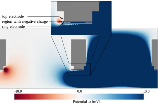
Figure 4.4.: Electrostatic potentials in free space caused by (a) Boersch phase plate or (b) twin aperture calculated using FiPy for a potentialU = 4V. To visualize the extent of the potentials a logarithmic, periodic color map has been chosen. Regions of interest for further evaluation are highlighted. Images on the right hand side show a close up on the phase plate structures in order to visualize the size of these structures.

(29)

surfaces, except those of the actual ring electrode, are set to a grounded potential φ = 0V, while the central ring electrode will be connected to a phase shifting potentialφ=U. Surfaces in the twin aperture designs (see Fig. 3.4b-f) are set to a grounded potential in an analogous way. Instead of a central ring the ring electrode in thex >0half plane will be set to a different potentialU.

In order to determine a potential dependent model of the phase shift due to the phase plates we solve Eq. 4.5 for different boundary conditions U ∈[0.05 V,10 V]. As indicated in Fig. 4.4 we will treat the potential φ in different regions of the phase plates separately. With Area A we will denote a subset of the xz plane which is limited by the ring electrode on potential U. Area B will be the remainder of the xz plane that an electron traveling along thez direction can pass. In case of the Boersch phase plate (see Fig. 4.4a) we regard the radial symmetry of the aperture and limit Area B to its parts on thex >0 half plane.

4.3. Modelling Phase Shift

In order to give an accurate expression for the electron wave function in the sample plane (see Fig. 2.3) in Chap. 5 one needs an analytical expression for the phase shift caused by the twin aperture in the C2 aperture plane. Therefore we will produce analytical models to reproduce the numerical results from the previous section4.2.

Furthermore we need an expression that relates the electrostatic potential caused by the phase plates with an actual phase shift. In doing so we will utilize the weak lens approximation which states that the potential of the phase plate has to be much smaller than the total energy of the accelerated electron. Thus one can assume that the electron passes through the phase plate in a straight line without getting deflected.

4.3.1. Electron Optical Background

The principle of electrostatic phase plates is subject to every course in quantum mechanics (compare Ref. [32]). One of the most simplest cases is the potential barrier in one dimension, which is located in the path of an electron wave. The electron has in front of and after the barrier the same wave length, but inside the barrier the wave length has a different value depending on the magnitude of the potential (see Fig. 4.5). Thus an electron traversing such a barrier is shifted in phase relative to an electron that travels through free space.

Figure4.5 illustrates a one dimensional potential barrier and the phase shift it causes to an electron wave passing through this barrier (green wave) relative to a wave travelling the same distance in absence of this barrier (red wave). The change in wave length and thus the phase difference between the two waves can simply be determined by solving the Schrödinger equation in case of non-relativistic electrons. The Schrödinger equation 4.24 and the wave length inside (Eq.4.25) and outside (Eq.4.26) of the barrier are given according to Ref. [32] as

(30)

d

U E

(a) Potential barrier.

−1.0 0.0 1.0 2.0 3.0

−1.0 0.0 1.0

x in multiples ofλ₁

Realpartofwavefunction

(b) Phase shift.

Figure 4.5.: One dimensional potential barrier of widthdand heightU (Fig.4.5a). The incoming electron has energyE, whereE > U. The real parts of the wave travelling through free space (red curve) and of the wave travelling through the potential barrier (green) are shown in Fig. 4.5b. The barrier is marked by a gray rectangle and has a width of1.5λ₁. The red wave has in the entire region a wave length of λ₁ = 2π/k₁ with k₁ = 1. The green wave has in front of and after the barrier also the wave length λ1. In the region of the barrier the wave length is altered to λ2 = 2π/k2 with k₂= 1.3.

d²ψ

dx² =−2m(E−V)

~² ψ (4.24)

λ2 =~π s

2

m(E−U) (4.25)

λ1 =~π r 2

mE, (4.26)

where the potential isV =U inside the barrier and V = 0 outside of the barrier, λ1 and λ2

are the wave length inside and outside of the barrier, m is the electron mass, E its kinetic energy and~is the reduced Planck constant.

As electrons are typically accelerated to energies of 200 – 300 keV in a TEM the expressions in equations4.25and4.26need to be determined from the relativistic equivalent to the Schrödinger equation, which is the Dirac equation. For sake of simplicity we will use the results as given in Refs. [5, 42]

λ₁ = hc

√2EE0+E² (4.27)

λ2 = hc

p2(E−U)E₀+ (E−U)², (4.28)

(31)

where h is the Planck constant, E₀ is the electron rest energy and c the speed of light in vacuum.

In analogy to light optics we introduce an electron-optical refractive indexn, which is defined as the ratio of the wave lengthλ₁ in a vacuum (and absence of external potentials) to the wave length λ2 in matter (or an external potentialV), as given in Ref. [42]

n(x, y z) = λ₁ λ2

= s

2(E−V(x, y z))E₀+ (E−V(x, y z))²

2EE0+E² , (4.29)

whereE is the kinetic energy of an electron,E0 its rest energy andV is the Coulomb potential in matter or — in this case — the external electrostatic potential caused by a phase plate. This expression can be simplified by assuming V E andE₀ (weak lens approximation)

n(x, y z) = 1− V(x, y z) E

E0+E

2E₀+E +. . . (4.30) Thus an optical path difference∆sand phase shiftϕcan be calculated⁴²by integrating along the path — which we define to be along the zaxis — of the electron

∆s= Z

z

(n(x, y, z)−1)dz (4.31)

ϕ(x, y) =2π

λ∆s= 2π λE

E0+E 2E₀+E

Z

z

V(x, y, z)dz, (4.32)

= π λE

E₀+E E₀+E/2

Z

z

φ(x, y, z)dz, (4.33)

where we have replaced a general potential V with the potential φ calculated in Sec. 4.2. In addition we have used a common convention for coordinate systems in electron microscopy.

The z axis is oriented along the optical axis of the microscope and xy planes are orthogonal to the optical axis.

In the following we will present the results of the previous calculations for the two different phase plate designs (compare Fig. 3.4) separately. In all subsequent calculations we will assume a primary energy of 200 keV and micrometers as unit of length. Furthermore we will assume that thez= 0 plane coincides with the bottom surface of the bottom layer of each phase plate design.

4.3.2. Boersch Phase Plate

Using the results from the finite element method calculations we will derive an analytical expression f for the phase shift ϕ(x) according to Eq.4.33, as we have only investigated a two dimensional cut plane.

Fig. 4.4a shows the electrostatic potential caused by the Boersch phase plate, where we have investigated a z range of [−10µm,11µm] in the FEM mesh. In the central region (x = [−0.9µm,0.9µm], Area A), which is a cross section of the ring electrode, the potential reproduces the results of a constant phase shift from Ref. [5] on first sight. In the outer annular

(32)

aperture area the potential has a different shape; one might compare it with the potential between two thin capacitor plates^a. As we will show subsequently this stray potential leads to a non-linear gradient in the phase shift (see Fig.4.6).

Fig. 4.6 shows the phase shift ϕ in the regions of interest (ROI) for boundary conditions U = 0.05V and U = 0.1V . The data obtained for Area A shows artifacts at the edge of the ROI. These artifacts will be ignored in the process of fitting functions to the data. All data obtained from numerical calculations is fitted with models. Fig. 4.6 also shows the used fit functions as red dashed lines.

4.3.2.1. Area A

The phase shift within the central ring electrode (Area A) of the Boersch phase plate (right hand side in Fig. 4.6) is in good agreement with previous results and can be approximated with a function only depending on U. Calculating mean value µ and standard deviation σ of the phase shiftϕ(x)inArea Aone gets for the ratioµ/σa value of8·10⁻³ meaning that the mean deviation from the mean valueµof data points on the right hand side in Fig. 4.6is negligible compared to the mean valueµ. This justifies the approximation ϕ_U(x, y) =ϕ_U(0,0).

In order to find a quantitative basis for the above approximation we will model the phase shift within the central ring electrode with a fit functionf that also takes into account non-constant contributions, which we choose to be a hyperbolic cosine as hyperbolic functions are typically part of solutions to differential equations like the Laplace equation,

f(x, U) =α(U) + cosh (β(U)·x)−1, (4.34) whereα andβ are fit parameters. The subtraction of1 takes into account that the phase shift has to vanish in absence of the potential

U→0limf(x, U) = 0. (4.35)

As we have solved the Laplace equation for values of the boundary conditions potentialU in the range[0.05 V,10 V]the dependence of the fit parametersα(U) and β(U) on the applied ring potentialU can be determined.

Fig. 4.7 shows the fit parameters α and β in dependence of the potential U. According to the model (see Eq.4.34) the parameter α describes the offset of the phase shift. The parameter shows a linear behavior. Regarding that the phase shift has to drop to zero for U = 0 the parameter itself cannot have a constant term.

The parameter β scales the hyperbolic cosine. β can be fitted with a square root function.

The expression for β cannot have a constant term in order to ensure that the phase shift becomes homogeneously zero forU = 0. Thus the fit parameters can be written as

aDistance between plates larger than plate diameter.