33
von Sara Bleninger
der Otto-Friedrich-Universität Bamberg
KriMI: A Multiple Imputation Approach for Preserving Spatial Dependencies
Imputation of Regional Price Indices
using the Example of Bavaria
Wirtschaftswissenschaften der
Otto-Friedrich-Universität Bamberg
Wirtschaftswissenschaften der Otto-Friedrich-Universität Bamberg
Band 33
2017
Preserving Spatial Dependencies
von Sara Bleninger
Imputation of Regional Price Indices
using the Example of Bavaria
Dieses Werk ist als freie Onlineversion über den Hochschulschriften-Server (OPUS; http://www.opus-bayern.de/uni-bamberg/) der Universitätsbiblio- thek Bamberg erreichbar. Kopien und Ausdrucke dürfen nur zum privaten und sonstigen eigenen Gebrauch angefertigt werden.
Herstellung und Druck: docupoint, Magdeburg
Umschlaggestaltung: University of Bamberg Press, Larissa Günther
© University of Bamberg Press, Bamberg, 2017 http://www.uni-bamberg.de/ubp/
ISSN: 1867-6197
ISBN: 978-3-86309-523-9 (Druckausgabe) eISBN: 978-3-86309-524-6 (Online-Ausgabe) URN: urn:nbn:de:bvb:473-opus4-502980 DOI: http://dx.doi.org/10.20378/irbo-50298
Diese Arbeit hat der Fakultät Sozial- und Wirtschaftswissenschaften der Otto-Friedrich-Universität Bamberg als Dissertation vorgelegen.
1. Gutachter: Prof. Dr. Susanne Rässler 2. Gutachter: Prof. Dr. Trivellore Raghunathan Tag der mündlichen Prüfung: 17.07.2017
Deutschen Nationalbibliographie; detaillierte bibliographische Informa-
tionen sind im Internet über http://dnb.d-nb.de/ abrufbar.
Diese Dissertation ist nicht nur das Resultat meines Aufwands, sondern das Ergebnis der Geduld ganz vieler Menschen. Ich durfte die größtmög- liche Unterstützung erfahren.
An erster Stelle muss ich mich bei meiner Doktormutter Susanne Rässler bedanken. Sie hat sich vor ungefähr fünf Jahren dafür mehr als verant- wortlich gefühlt, dass ich meine Dissertation an der Universität Bamberg nicht nur einfach schreiben kann, sondern auch eine gute Betreuung und ein interessantes Thema habe. Sie hat ein Umfeld geschaffen, in dem ich mich frei entfalten konnte und mich sehr wohl fühle.
Zu diesem Umfeld gehören insbesondere meine nun ehemaligen Kolle- gen am Lehrstuhl. Besonders möchte ich mich dabei bei Alexandra Trojan bedanken, die mit mir zusammen in dem Projekt zu regionalen Preisen promoviert. Unseren kleinen privaten Workshop in unserem Esszimmer habe ich sehr genossen. Zudem möchte ich mich bei Thorsten Schnapp für seine andauernde R-Hilfe bedanken. Er hat eigentlich fast immer für meine R-Probleme Lösungen und Antworten gehabt. Das Gleiche gilt für Florian Meinfelder. Seine Hilfe war der Startpunkt für viele meiner R- Programmierungen. Sören Abbenseths geduldige Hilfe bei der Aufberei- tung der Preisdaten darf nicht unerwähnt bleiben.
Rachel und Jenny schulde ich Dank für ihre unendliche Geduld, meine Ar- beit auf sprachliche Mängel hin zu korrigieren. Sie haben das beide sehr ausdauernd gemacht und auch ertragen, was ich ihrer schönen Mutter- sprache in manchen Fällen angetan habe.
Aber die größte Hilfe bei allem war Philipp. Es ist von unschätzbarem
danken, dass er so ein Sonnenschein ist, dass ich nebenbei meine Arbeit fertig schreiben konnte.
Zuletzt muss ich noch die Menschen im Hintergrund erwähnen, ohne de- ren Unterstützung ich das alles nicht geschafft hätte. Das sind auf jeden Fall meine beiden Eltern, die sich für mich immer ein Bein ausgerissen haben, die sich nie darüber beschwert haben, dass ich jahrelang studiert habe, die alles in jeglicher Hinsicht unterstützt haben, die immer da sind.
Auch meiner Schwiegermama Susi gilt mein Dank, vor allem dafür, dass
sie sich immer so toll um Jakob kümmert. Es ist aber auch schön, dass sie
so stolz auf mich ist und bei Gott und der Welt mit ihrer Schwiegertochter
angibt. Meinem Schwiegervater Manfred und Andrea muss ich vor allem
für die tolle Unterstützung während meines Statistik-Studiums in Mün-
chen danken, aber auch für die vielen tollen Gespräche und das Interesse.
Inhaltsverzeichnis
1 Introduction 13
2 Multiple Imputation 17
2.1 Describing the Missingness Mechanism . . . . 18
2.2 Introduction to Multiple Imputation . . . . 20
2.2.1 Reasoning Multiple Imputation . . . . 21
2.2.2 More than a Little Inaccuracy . . . . 22
2.2.3 Getting Multiple Draws . . . . 24
2.2.4 The Gibbs-Sampler . . . . 29
2.2.5 Monotone Distinct Structure . . . . 32
2.3 Combining Multiple Values . . . . 34
2.3.1 Multiple Imputation Estimation . . . . 34
2.3.2 Multiple Imputation Variance Estimation . . . . . 36
2.4 Requirements . . . . 39
2.5 Advantages and Disadvantages . . . . 40
3 Kriging 42 3.1 Introduction into One-dimensional Kriging . . . . 43
3.2 The Method of Kriging . . . . 44
3.2.1 Continuous Kriging . . . . 45
3.3 Prediction . . . . 48
3.3.1 Simple Kriging Predictor . . . . 49
3.3.2 Ordinary Kriging Predictor . . . . 52
3.3.3 Universal Kriging Predictor . . . . 55
3.3.4 Comparison by MSPEs . . . . 62
3.3.5 Bayesian Prediction . . . . 63
3.4 The Correlation Structure . . . . 67
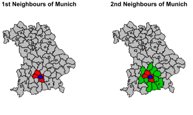
3.4.1 Neighbourships . . . . 68
3.4.2 Correlation Functions . . . . 69
3.4.4 Maximum Likelihood (ML) . . . . 74
3.4.5 Restricted Maximum Likelihood . . . . 75
3.4.6 Bayesian Estimation . . . . 78
3.4.7 Variogram . . . . 78
4 KriMI: Multiple Imputation Using Kriging 81 4.1 Predicting Using Mixed Modelling . . . . 81
4.1.1 The Model . . . . 82
4.1.2 Bayesian Modelling . . . . 85
4.1.3 Criticism of Mixed Modelling of Kriging for Multi- ple Imputation . . . . 89
4.2 Predicting Using P-Splines . . . . 90
4.2.1 P-Splines . . . . 91
4.2.2 Bayesian P-Splines . . . . 94
4.2.3 Kriging as a P-Spline . . . . 99
4.2.4 Predictions . . . 103
4.2.5 Choosing the Knots . . . 103
4.2.6 Bayesian Modelling and the Gibbs-Sampler . . . . 104
4.2.7 Other Approaches for Including Nonparametric Me- thods . . . 106
5 Prices, Price Indices and the Official Price Statistics in Germany 111 5.1 Prices . . . 111
5.2 Price Indices . . . 111
5.3 Computing with Price Measure Numbers and Price Indices 114 5.4 Price Statistics in Germany . . . 115
5.4.1 German Price Survey . . . 115
5.4.2 The Consumer Price Index (CPI) . . . 116
6 Regional Price Levels 119 6.1 Regional Price Indices . . . 120
6.1.1 Definition of Bilateral Regional Price Indices . . . 120
6.1.2 Axioms for Regional Price Indices . . . 125
6.1.3 Multilateral Regional Price Index . . . 127
6.2 A Shopping Basket for Regional Price Indices . . . 128
6.2.1 Products Should Be Comparable . . . 129
6.2.2 Products Must Be Available in Every Region . . . . 131
6.2.3 Products Must Have Different Prices . . . 133
6.2.4 Regional Market Basket Must Be Representative . 134 6.3 The Price Data . . . 135
6.4 Influencing Factors of the Price Level: A Regression Model for Regional Prices . . . 138
6.4.1 Discussion of Studies on Regional Price Levels . . 138
6.4.2 The Data for the Influencing Factors . . . 157
6.4.3 Identifying the Influencing Factors on Regional Pri- ces . . . 157
7 Prediction of Regional Prices 164 7.1 Single Imputation . . . 164
7.1.1 Regression Models on Regional Prices . . . 164
7.1.2 Single Imputation by Conditional Means . . . 173
7.2 Universal Kriging . . . 177
7.2.1 The Universal Kriging Model . . . 177
7.2.2 Estimating the Variance Parameters . . . 178
7.2.3 Estimating the Parameters . . . 179
7.2.4 Single Imputation by Kriging . . . 180
7.3 Multiple Imputation . . . 183
7.3.1 Prior, Posterior, and Full Conditionals . . . 184
7.3.2 Gibbs-Sampler . . . 185
7.3.3 Multiple Imputation by Linear Regression . . . 186
7.4 KriMI: Multiple Imputation by Kriging . . . 189
7.4.1 KriMI by the Mixed Model Approach: Gibbs-sampler 190 7.4.2 KriMI by the Mixed Model Approach: Results . . . 191
7.4.3 KriMI by Baysian P-Splines: Priors, Posterior, Full
Conditionals, and Gibbs-sampler . . . 193
8 Outlook 200
A Proofs and Computation 214
A.1 R-packages used . . . 214
A.2 Multiple Imputation . . . 216
A.3 Kriging . . . 223
A.3.1 Simple Kriging . . . 223
A.3.2 Ordinary Kriging . . . 226
A.3.3 Universal Kriging . . . 230
A.4 Full Conditionals of the NIG Regression Model . . . 234
A.5 Full Conditionals of the KriMI Model . . . 236
B Price Data 240 C Outputs and Results 250 C.1 Outputs of the Linear Regression Estimation by COICOP- Classification . . . 250
C.2 Results of the Price Index Imputation . . . 257
C.2.1 Single Imputation . . . 257
C.2.2 Universal Kriging . . . 260
C.2.3 Multiple Imputation . . . 262
C.2.4 KriMI by Mixed Modelling . . . 265
C.2.5 KriMI by P-Splines . . . 268
Abbildungsverzeichnis
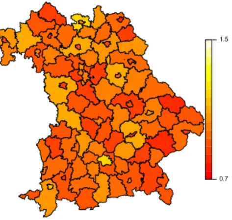
1 First and Second Neighbours of Munich . . . . 69 2 Example of a Variogram . . . . 79 3 Regional Lowe Price Index by Single Regression Imputation 174 4 Variogram of the Regional Lowe Price Index by Single Re-
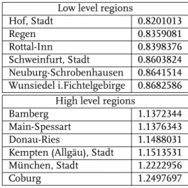
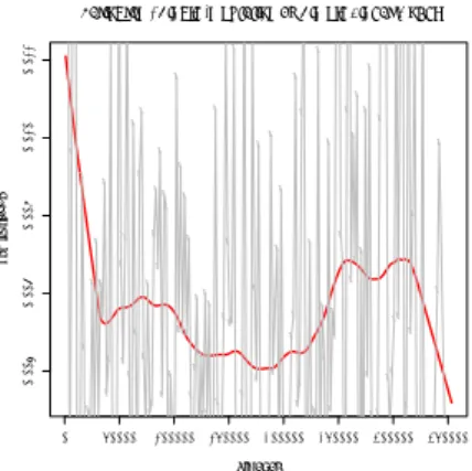
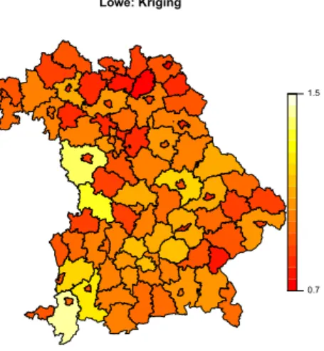
gression Imputation . . . 176 5 Regional Lowe Price Index by Kriging . . . 181 6 Variogram of the Regional Lowe Price Index by Kriging . . 183 7 Regional Lowe Price Index by Multiple Imputation . . . . 187 8 Variogram of Regional Lowe Price Index by Multiple Im-
putation . . . 189 9 Regional Lowe Price Index by KriMI with Mixed Modelling 192 10 Variogram of the Regional Lowe Price Index by KriMI with
Mixed Modelling . . . 194 11 Regional Lowe Price Index by KriMI with P-Splines . . . . 197 12 Variogram of the Regional Lowe Price Index by KriMI with
P-Splines . . . 199
Tabellenverzeichnis
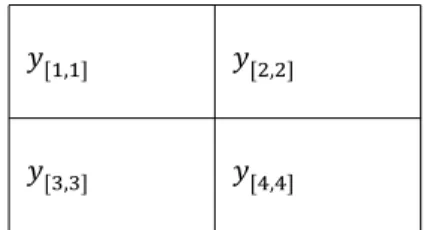
1 KriMI Example 1 . . . . 83
2 KriMI Example 2 . . . . 84
3 Summary of Influencing Factors Mentioned in Literature 156 4 Influencing Factors Taken into Account . . . 163
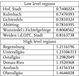
5 Highprice and Lowprice Regions by Single Regression Im- putation . . . 175
6 Highprice and Lowprice Regions by Kriging . . . 182
7 Highprice and Lowprice Regions by Multiple Imputation . 188 8 Highprice and Lowprice Regions by KriMI with Mixed Mo- delling . . . 193
9 Highprice and Lowprice Regions by KriMI with P-Splines 198 10 Data Used in the Analysis . . . 240
11 Results for Food and Non-alcoholic Beverages . . . 250
12 Results for Alcoholic Beverages, Tobacco, and Narcotics . 251 13 Results for Clothing and Footware . . . 251
14 Results for Housing, Water, Electricity, Gas and other Fuels 252 15 Results for Furnishings, Household Equipment and Rou- tine Household Maintenance . . . 252
16 Results for Products and Services of Health . . . 253
17 Results for Transport . . . 253
18 Results for Communication . . . 254
19 Results for Recreation and Culture . . . 254
20 Results for Education . . . 255
21 Results for Restaurants and Hotels . . . 255
22 Results for Miscellaneous Goods and Service . . . 256
1 Introduction
In the middle of every month the German Federal Statistical Office relea- ses the new consumer price index reporting the current cost of living of a typical German household. Every month it is reported that the amount that a German household has to pay for a typical market basket changed at a certain degree given as a percentage number. The German media month- ly report the current inflation rate for Germany based on this percentage number, which is called price index. Even though reported for years, every month there is still an important question left unanswered: Do price levels differ among regions? The public attention mostly focuses on the national inflation representing the change of the price level over time. A spatial point of view remains unobserved.
Exploring the regional disparities should be of great public interest. It goes beyond answering the question where we have to pay more or less. There are a lot of public transfer payments that are given according to needs. Of course the costs of these needs measured in money depends on the local price level. Recipients of the public transfer payments have to pay more for their livelihood in a high price region than persons living in a low price region. Also the salary of civil servants should be aligned to the local cost of living. For this reason, a Bavarian policeman took the state to court as he wanted his salary adjusted for the region he lived in. This lawsuit was one of the rare events when regional cost of living appeared in the public arena. The court refused the lawsuit.(BVerfG, 2007)
In science the question of regional price disparities plays a bigger role than
in public discourse. There are a lot of publications about regional price le-
vels. We are going to discuss some of them later. Economic and social
scientists need regional cost of living for adjusting all kinds of income and
is analysing people’s income, it is not the nominal amount which is of in- terest, but what we can buy for it. The latter is the real value, which is the nominal income adjusted for the regional price level.
Contrary to the need of regional price indices, there are not much data available on that high level of fragmentation. There are two relevant stu- dies surveying regional data on prices in Germany, i.e. Rostin (1979) and Ströhl (1994), but these are rather old. The newer study of Ströhl (1994) only inspects prices in 50 cities, which is not enough for an investigation of regional price disparities. For these reasons there have been efforts to extend the data base by regression imputation, e.g. Roos (2006), or even with multiple imputation, e.g. Blien et al. (2009).
This thesis is written in the context of a project group with the objective of solving the various problems associated with computing regional price indices. There are several tasks to be solved: a regional price index needs to be developed, price data for all regions need to be surveyed or predic- ted, there are special problems with housing costs etc. For this reason, this thesis only plays a part in solving the various problems involved with ac- quiring a regional cost of living value. However, it is complete in providing statistical models to generate predictions of the prices in unsurveyed regi- ons.
The single imputation by regression generates good results, i.e. means
are correct in the long run. However, the interest is not to analyse regional
prices itself, but to use the regional price level for subsequent studies. As
regression imputation always underestimates variances of estimators, all
succeeding significance levels are seriously biased. Donald B. Rubin de-
veloped a method to overcome the problem of underestimating variances
by using Bayesian theory.(Rubin, 1987) The uncertainty brought in by the
missing data is represented by imputing more times than once. Here, we
define the regions where no price data were surveyed as missing values.
The problem of unknown regional price levels becomes a problem of mis- sing data which can be solved with missing data techniques, i.e. multiple imputation. In the second chapter we will introduce the argumentation and method of multiple imputation.
Actually, the problem of predicting the prices in unsurveyed regions is a matter of geostatistics. The models of geostatistics allow the modelling of spatial dependencies and inter-dependencies of neighbouring regions.
Probably the prices in neighbouring regions are dependent on each other, making such a spatial modelling necessary. Geostatistics keeps a group of models at hand which are developed for predicting spatial dependent observations: kriging. In the third chapter, we will introduce kriging. The focus is on modelling spatial dependencies via correlation functions and covariances.
Both approaches solve one problem that we face when predicting unsur-
veyed regional prices. Multiple imputation allows proper inferences in suc-
ceeding statistical analysis. Kriging preserves spatial dependencies of the
predicted values. If we want both, it seems a promising idea to combine
both methods to get spatially dependent values for the unobserved pri-
ces that allow succeeding inference. In chapter 4 we derive two ways to
implement kriging into the multiple imputation scheme. First, kriging is
modelled as a mixed model where spatial dependencies are modelled in
the variance-covariance matrix. The Bayesian formulation of the formed
mixed model is then used to generate multiple imputations. Second, the
familiarity of kriging to P-spline smoothing is exploited to derive a model
that is closer to the given data. Again the Bayesian formulation is used to
implement kriging into the multiple imputation model. We call these two
models KriMI models as they are an amalgamation of kriging and multi-
ple imputation.
In the seventh chapter we use all introduced statistical models to predict the unobserved prices in Bavarian regions. The Bavarian State Office for Statistics provided the data that are surveyed for the official consumer price index on a regional level. There are huge blank areas in the map of regio- nal prices. For this reason the Bavarian data are a prime example to test our models. However, before we estimate and predict the missing price data, a short introduction to prices and price indices is given, as we need to know the observation object. We also mention briefly the special pro- blems of regional price indices. For all statistical models we need to know relevant influencing factors. These are also derived in chapter 5. After this we create a baseline by imputing regional prices with a simple regression approach. Following sections identify the missing price data by multiple imputation and kriging to use the models in their pure form. In a final step we use the developed KriMI models for a multiple imputation of regional prices that preserves spatial dependencies. For all methods used, we report the regional price indices of the Bavarian regions.
All analyses and all graphs, including the maps, are made using the sta-
tistical software R Core Team (2015a), Belitz et al. (2015), and the geo-
information system GRASS Development Team (2012). We used several
packages in R. All references for those R-packages can be found in the
appendix.
2 Multiple Imputation
Multiple imputation is a method of handling missing data problems. (Zha- ng, 2003) As in single imputation, missing values are replaced by sensible values, but the replacement is done several times as
” the inserted values should reflect variation within a model as well as variation due to the va- riety of reasonable models. “ (Rubin, 1978). The aim is to still have a statis- tically valid inference in the case of missing data: In single imputation a correct variance imputation is no longer possible due to the replacements.
Multiple imputation by contrast uses the differences between the several replacements to correct variance estimation to allow a valid statistical in- ference. Moreover, multiple imputation allows valid statistical inference in the case where the data analyst and the data manager are not the same person.(Rubin, 1996) These two arguments allow the use of multiple im- putation in the case of missing regional price information.
Other techniques for incomplete data are based on the likelihood approach (e.g.the EM algorithm, the random effects model), but are inferior for the reason of greater complexity.(Zhang, 2003) As the problem of regionalised price indices can only be solved by providing completed data, imputation methods should be preferred to the likelihood based methods.
Zhang (2003) names three steps with which to conduct data analysis with multiple imputation:
1. Create 𝑚 > 1 completed data sets by filling in each missing value 𝑚
times using a proper imputation model. Following the description
of Schafer (1999) to get the multiple draws it becomes clear that it is
not that easy:
• Second, according to Bayesian statistics, a prior has to be spe- cified for the model parameters which are unknown, and
• 𝑚 independent draws from the conditional distributions are simulated.
2. Conduct a complete data analysis on each of the 𝑚 filled data sets.
3. Combine the statistics from step two by the combining rule.
Similarly, Rubin (1988) subsumes multiple imputation:
” As its name sug- gests, multiple imputation replaces each missing value by a vector com- posed of 𝑀 ≥ 2 possible values. The 𝑀 values are ordered in the sense that the first components of the vectors for the missing values are used to create one completed data set, the second components of the vectors are used to create the second completed data set and so on; each completed da- ta set is analysed using standard complete-data methods. “ (Rubin, 1988) A similar introduction can be found in Schafer (1999). Here, we emphasise step one while leaving the second step completely up to the researcher of regional prices. For step three, we give a short instruction. To do so we first describe the problem: In the next section we attend to the missingness me- chanisms. Subsequently, a short insight is given into reasoning multiple imputation, followed by the combining rules. After having described the main body of multiple imputation, we spend some time on the details.
2.1 Describing the Missingness Mechanism
Before presenting a solution of missing values, we need to describe the
problem itself. Ordinarily, there are data that are not observed when being
collected. These data are missing. We distinguish three kinds of missing-
ness described in this chapter.
Defining the variable R, with
𝑟 = 1 if 𝑦 is observed 0 if 𝑦 is missing
with 𝑖 = 1, … , 𝑛 denoting observations and 𝑗 = 1, … , 𝑝 denoting variables.
The probability distribution belonging to 𝑅 is 𝑃 (𝑅|𝜑, 𝑌) with the parame- ters 𝜑 and the data matrix 𝑌. The joint distribution of data and missingness indicator is (Zhang, 2003):
𝑃 (𝑌, 𝑅|𝜃, 𝜑) = 𝑃 (𝑌|𝜃) 𝑃 (𝑅|𝜑, 𝑌)
where 𝜃 is a parameter or parameter vector for the data 𝑌. We denote the missing data as 𝑌 meaning that these are the cases where 𝑟 = 0.
Observed data are 𝑌 where 𝑟 = 1.
According to Rubin (1987), Zhang (2003), and several other authors, the following missingness mechanisms can be distinguished:
1. Missing Completely at Random (MCAR)(Rubin, 1987, Zhang, 2003) 𝑃 (𝑅|𝜑, 𝑌) = 𝑃 (𝑅|𝜑)
” The probability of missing data on one variable is not related to the value of that variable or other variables in the data set. “ (Patrician, 2002) By a comparison of the data of respondents to the data of non- respondents, the assumption of MCAR can be verified.(Patrician, 2002)
2. Missing at Random (MAR)(Rubin, 1987, Zhang, 2003)
𝑃 (𝑅|𝜑, 𝑌) = 𝑃 (𝑅|𝜑, 𝑌 )
The probability of missingness of one value does not depend on the variable that is missing itself, but may depend on other variables in- cluded in the data set.(Patrician, 2002) According to Patrician (2002), the assumption MAR cannot be tested. MAR is relative to the varia- bles included in the data set. All variables that are responsible for the missingness must be considered in the data set.(Schafer and Olsen, 1998)
3. Not Missing at Random (NMAR)(Rubin, 1987, Zhang, 2003) 𝑃 (𝑅|𝜑, 𝑌) ≠ 𝑃 (𝑅|𝜑)
Following, we assume at least MAR, even though there are also possibili- ties to handle NMAR.(Rubin, 1987)
2.2 Introduction to Multiple Imputation
One way to identify appropriate values for missing data is multiple im- putation (MI) introduced by Rubin (1987) and among others described in Little and Rubin (2002). The underlying idea is to impute 𝑚 credible values for each missing value to create 𝑚 filled data sets instead of imputing just one value to get one filled data set. Doing so, MI has all the advantages of single imputation thereby solving the problem of variances.
Multiple imputation uses the available information to find sensible values
replacing the missing data. These are the observed data and information
due to the data model (prior). A model connecting observed and unobser-
ved values is needed to find proper imputations.(Rubin, 1987) This is done
in the following subsubsection. In subsubsection 2.2.3 we describe how to
find these proper values for missings, followed by a short insight into the
special case of a monotone distinct missingness structure. We do not de- scribe how to combine the multiple data sets until the following section.
2.2.1 Reasoning Multiple Imputation
Explicitly, MI means to repeatedly fill in values for the missing data 𝑌 . In the end, we get: 𝑌 , ; 𝑌 , ; ⋯ , 𝑌 . The different sets of missing values are drawn from the posterior predictive.(Rubin, 1996) Rubin (1987) justifies this using the Bayesian Theory. One bunch of replacements for missings are got by drawing from the posterior distribution employing the Bayesian theory. As posteriors often cannot be computed, proper va- lues for unobserved data are found by iterative simulation methods.(Little and Rubin, 2002) Due to drawing, Schafer (1997) states:
” Like parameter simulation, multiple imputation is a Monte Carlo approach to the analy- sis of incomplete data. (...) solving an incomplete-data problem by repea- tedly solving the complete data version. “ (Schafer, 1997, S.104) Thereby, Bayesian theory is justification, theoretical background and prescription of MI.(Rubin, 1987)
In this section we first show the reason why inferential statistics can be done using imputed data instead of using the complete data. This is the justification and theoretical background of MI.
Little and Rubin (2002) and other authors of MI consider the complete data posterior:
𝑃(𝜂|𝑌 , 𝑌 , 𝑋) ∝ 𝑃(𝜂)𝐿(𝜂|𝑌 , 𝑌 , 𝑋). (1)
In compliance with the three Bayes Postulates and especially the Bayes Co-
rollary, inferences shall only be made on the basis of the complete data pos-
𝑃 (𝜂|𝑌, 𝑋) = 𝑃(𝜂|𝑌 , 𝑌 , 𝑋).(Rüger, 1999) Until now, we only
formulated classic Bayesian inference. Returning to the missing data pro- blem, it becomes clear that we cannot observe the complete-data posterior 𝑃(𝜂|𝑌 , 𝑌 , 𝑋) due to the missing data. As we know the observed-data posterior, the relationship between observed-data-posterior and complete- data-posterior needs to be drawn (Little and Rubin, 2002, Zhang, 2003):
𝑃 (𝜂|𝑌 , 𝑋) = 𝑃 (𝜂, 𝑌 |𝑌 , 𝑋) 𝑑𝑌
= 𝑃 (𝜂|𝑌 , 𝑌 , 𝑋) 𝑃(𝑌 |𝑌 , 𝑋)𝑑𝑌 (2) First the rule of Total Probability is used to integrate 𝑌 out and, in a second step, again the Bayes Rule is employed.
Rubin (1987) summarises formula 2 in result 3.1: ” Averaging the Com- plete-Data Posterior Distribution of (...) [𝜂] over the Posterior Distribution of 𝑌 to obtain the Actual Posterior Distribution of (...) [𝜂]“ (Rubin, 1987, S.82). Rubin (1987) states that it ” can be applied to simulate the actual pos- terior distribution of 𝑄 (here: 𝜂) using repeated draws from the posterior distribution of the missing values. “ (Rubin, 1987). As no additional infor- mation should be added to the estimation than the observed data and the prior knowledge expressed in the prior distribution, inferences should on- ly be made on the basis of the observed data posterior. The derived link between observed-data posterior and complete-data posterior shows that this still holds if inference is made on the multiply imputed data.
Moreover, the integral 2 justifies Rubin’s combining rules described later on in section 2.3, too.(Rubin, 1996) The integral is just approximated by the respective sum.
2.2.2 More than a Little Inaccuracy
Before turning to the sampling mechanism for the replacement of mis-
sing values, we need to confess a little inaccuracy. Correctly, Rubin (1987)
adds in every formula mentioned above an indicator for inclusion to the survey 𝐼 and an indicator for response 𝑅. This is because of the statistical validity of the estimates.(Rubin, 1996) Rubin (1987) shows that it is not necessary to condition on the inclusion indicator under the assumption of an ignorable sampling mechanism. More importantly, he also shows the same for the indicator of non-response 𝑅 when the response mechanism is ignorable. The importance of this is due to the ignorance of most stu- dies in respect to the possibility of non-response. Rubin (1987) states that most surveys just ignore non-response and, therefore, do not include con- ditioning on 𝑅. However, the assumption of ignorable non-response still remains even if 𝑅 is just ignored. To keep the necessary assumptions in mind, we note this inaccuracy.
However, the result implies more than just a simplification of notification.
In ordinarily used statistical models the most employed assumption is the assumption of independent and identical distribution. For this very com- mon and widely used assumption, Rubin (1987) states in his Result 3.4:
” The Equality of Completed-Data and Complete-Data Posterior Distributi- ons When Using i.i.d. Models.“(Rubin, 1987)
𝑃 (𝜂|𝑋, 𝑌 , 𝑅 ) = 𝑃 (𝜂|𝑋, 𝑌 )
The subscipt 𝑖𝑛𝑐 indicates whether the case was included in the study or not, 𝑖𝑛𝑐 = (𝑜𝑏𝑠, 𝑚𝑖𝑠). We show the proof of result 3.4, i.e. the equality of completed-data and complete-data posterior under the assumption of i.i.d.
in the appendix.
Result 3.4 reasons that the same statistics may be computed on basis of the
completed-data sets as would be done on the basis of the complete-data set.
tics can be computed, is it possible to estimate them by combining several completed data sets.
Later on, we assume ignorable non-response in the first instance. For all non-ignorable cases, this reformulation using Bayes’ Rule is very useful:(Ru- bin, 1987)
𝑃 (𝜂|𝑋, 𝑌 ⎭ ⎪ ⎪ ⎬ ⎪ , 𝑅 ⎪ ⎫ )
completed-data posterior
= 𝑃 (𝜂|𝑋, 𝑌 ⎭ ⎪ ⎬ ⎪ ⎫ )
complete-data posterior
𝑃 (𝑅 |𝑋, 𝑌 , 𝜂)
⎭ 𝑃 (𝑅 ⎪ ⎪ ⎬ |𝑋, 𝑌 ⎪ ⎪ ⎫ )
adjustment factor
, (3)
In the case of ignorable non-response, the adjustment factor becomes 1, which refers to the equality of both in that case (see Rubin’s Result 3.3), otherwise the adjustment factor needs to be employed. According to Rubin (1978) ” the trick is to tie the parameters for the different groups of units together so that the values we do see tell us something about the values we do not see. “ (Rubin, 1978)
2.2.3 Getting Multiple Draws
However, we did not clarify yet how to actually get multiple replacements for the missing values. A short insight is given in this chapter. Let’s start again with the underlying idea of drawing 𝑚-times from the posterior dis- tribution 𝑃 (𝑌 |𝑋, 𝑌 ) to get 𝑚 sets of imputations 𝑌 , ; 𝑌 , … , 𝑌 and 𝑚 completed data sets 𝑌 , 𝑌 , … , 𝑌 . (Rubin, 1987) Now we are engaged in creating one completed data set by finding sensible replace- ments for the missing values.
” [I]n order to insert sensible values for missing data we must rely on some model relating unobserved values to observed values “ (Rubin, 1978) which is done when drawing from the posterior predictive which displays
” the
sensitivity of inferences to reasonable choices of models “ (Rubin, 1978).
Therefore, the 𝑚 draws should be made from the posterior of 𝑌 which can be reformulated by the use of the rule of Bayes and the law of total probability (Rubin, 1987):
𝑃 (𝑌 |𝑋, 𝑌 ) = 𝑃 (𝑋, 𝑌)
∫ 𝑃 (𝑋, 𝑌) 𝑑𝑌
It is sufficient to consider 𝑃 (𝑋, 𝑌) to determine the model for the data.(Ru- bin, 1987, 1978) The aim is to formulate the prior knowledge of the da- ta.(Rubin, 1978)
Then Rubin (1987) reformulates to get a connection to the parameter 𝜃 which is the parameter describing the distribution of 𝑌 for using MCMC methods to simulate the complex distribution:
𝑃 (𝑋, 𝑌) = 𝑃 (𝑋, 𝑌|𝜃) 𝑃 (𝜃) 𝑑𝜃
= 𝑓 (𝑋 , 𝑌 |𝜃) 𝑃 (𝜃) 𝑑𝜃
= 𝑓
|𝑌 |𝑋 , 𝜃
|𝑓 (𝑋 |𝜃 ) 𝑃 (𝜃) 𝑑𝜃
The last step using the rule of Bayes again does not seem necessary at the beginning, but as stated in Result 5.1 it greatly facilitates getting multiple imputations. It is not necessary to specify a model for the parameters. It is sufficient to model the conditional parameters and data models.(Rubin, 1987) For example, this can be done by simple regression.
After having specified the data model, we need to find a way to draw sensi-
ble values for the missing data. Starting again with the posterior predictive,
which is the only distribution for drawing missing values, another facto-
risation is helpful. It can be found, among others, in Rubin (1987) and Zhang (2003):
𝑃 (𝑌 |𝑌 , 𝑋) = 𝐸 [𝑃(𝑌 |𝑌 , 𝑋, 𝜃)]
= 𝑃(𝑌 |𝑌 , 𝑋, 𝜃)𝑃(𝜃|𝑌 , 𝑋)𝑑𝜃 (4) The posterior predictive distribution now is factorised into:
1. conditional predictive distribution of 𝑌 : 𝑃(𝑌 |𝑌 , 𝑋, 𝜃) 2. observed data posterior distribution of 𝜃: 𝑃(𝜃|𝑌 , 𝑋)(Zhang, 2003) To define the distribution of 𝑌, we need to determine a prior 𝑃(𝜃) and a distribution for the data 𝑃(𝑌 |𝜃). Schafer (1997) also uses this expecta- tion over the parameter 𝜃. He emphasises that a proper Bayesian multiple imputation uses the averaging over the observed data posterior to reflect the uncertainty of missing data given the parameters and the uncertainty of the model parameter themselves.(Schafer, 1997)
Using the Integral 4, Schafer (1999) describes the drawing scheme to get one set of imputations: first, a random draw of the parameter following the observed data posterior shall be done. Second, determined by the draw of the parameter, the missing values 𝑌 shall be drawn from the condi- tional predictive distribution.(Schafer, 1999)
According to Zhang (2003) and Schafer (1999) it is rarely possible to ex-
press the posterior predictive in closed form or to draw from it. However,
he also states it is often easy to obtain the conditional predictive. This rea-
sons the drawing mechanisms described later on. The drawing mechanis-
ms are mostly MCMC-methods.(Schafer, 1999) In a lot of cases it is still
quite difficult to simulate the draws from the observed data posterior. For
this reason Rubin (1987) proposes a simplification in his Results 5.1 and
5.2. First, we should quote the
Result 5.1 ” The Imputation Task with Ignorable Nonresponse “ : ” Given 𝜃, the 𝑌
,are a posteriori independent with distribution depending on 𝜃 only through 𝜃
|: “ (Rubin, 1987)
𝑃 (𝑌 |𝑋, 𝑌 , 𝜃) = 𝑃 𝑌
,|𝑋 , 𝑌
,, 𝜃
|The proof is given in the appendix. In a lot of cases, it is much easier to compute 𝑃 𝑌
,|𝑋 , 𝑌
,, 𝜃
|than to compute 𝑃 (𝑌 |𝑋, 𝑌 , 𝜃).
Just bear the possibility of linear regression in mind.
According to this result, it is possible to take 𝑃 𝑌 |𝑋, 𝑌 , 𝜃
|into ac- count instead of the unconditioned 𝑃 (𝑌 |𝑋, 𝑌 , 𝜃). Now, it all breaks down to specify 𝑃 𝑌 |𝑋, 𝑌 , 𝜃
|, which can often be simulated by MCMC methods. If the missings are ignorable, standard Bayes methods can be used.(Rubin, 1987) Zhang (2003) recommends simulating the ob- served data posterior distribution by a Gibbs-Sampling or to use the Pre- dictive Model Method as alternative to the sampling.
In turn, Rubin (1987) exposes a simplification. He states this in Result 5.2:
” The Estimation Task with Ignorable Nonresponse When 𝜃
|and 𝜃 Are a Priori Independent “ :
” Suppose 𝜃
|and 𝜃 are a priori independent 𝑃𝑟 (𝜃) = 𝑃𝑟 𝜃
|𝑃𝑟 (𝜃 )
Then they are a posteriori independent; moreover, the posterior distributi- on of 𝜃
|involves only (a) the specifications 𝑓
|(⋅|⋅) and 𝑃𝑟 𝜃
|and
𝑌
of independence, it is possible to use only 𝑃 𝜃
||𝑋, 𝑌 , which simpli- fies computation:
1𝑃 𝜃
||𝑋, 𝑌 (5)
= ∏ ∫ 𝑓
|𝑌 |𝑋 , 𝜃
|𝑑𝑌
,𝑃 𝜃
|∫ ∏ ∫ 𝑓
|𝑌 |𝑋 , 𝜃
|𝑑𝑌
,𝑃 𝜃
|𝑑𝜃
|(6) According to Rubin (1987), it is sufficient to multiply over the units with observed values. A further simplification is the case of univariate 𝑌 as Rubin (1987) states in Result 5.3: ” The Estimation Task with Ignorable Nonresponse, 𝜃
|and 𝜃 a Priori Independent, and Univariate 𝑌 If 𝜃
|and 𝜃 are a priori independent and 𝑌 is univariate so that the respondents have 𝑌 and the non-respondents are missing 𝑌 , the posterior distribution of 𝜃
|involves only the respondents.“ For this reason, the conditional posterior becomes (Rubin, 1987):
𝑃 𝜃
||𝑋, 𝑌 = ∏ 𝑓
|𝑌 |𝑋 , 𝜃
|𝑃 𝜃
|∫ ∏ 𝑓
|𝑌 |𝑋 , 𝜃
|𝑃 𝜃
|𝑑𝜃
|(7) To subsume the last section, these steps were discussed:
1. 𝑌
,are a posteriori independent.
2. The distribution of 𝑌
,only depends on 𝜃 through 𝜃
|. 3. 𝑃 𝜃
|and 𝑃 (𝜃 ) are a priori independent.
In this case we only have to specify 𝑓
|, 𝑃 𝑌|𝑋, 𝜃
|and data from ob- served units. In the case of univariate 𝑌 we only need the data of the re- spondents.
1
Jackman (2009) shows the same for regression models which is the main reason why
Rubin’s result makes computations easier.
2.2.4 The Gibbs-Sampler
The basic rule to get multiple draws for multiple imputation is stated in Conclusion 4.1 by Rubin (1987):
” If imputations are drawn to approximate repetitions from a Bayesian posterior distribution of 𝑌 under the posi- ted response mechanism and an appropriate model for the data, then in large samples the imputation model is proper. “ (Rubin, 1987) Therefore, the drawing scheme should be based on a Bayesian idea to preserve cor- rect variance estimation.(Rubin, 1987) Zhang (2003) describes the sam- pling idea to create multiple draws. First, draw 𝜃 from its observed data posterior distribution given in equation 4. Then draw one set of 𝑌 from 𝑃 𝑌 |𝑌 , 𝑋, 𝜃 . In order to create 𝑚 sets of missing data, repeat this 𝑚 times independently.(Zhang, 2003)
Under the assumption of normality the imputation problem can be solved by using a linear regression where the missing values are the predictions.
The parameters of the regression are the distributional parameters being drawn to assess the model uncertainty.(Zhang, 2003)
Define 𝑋 as the data matrix with the variables observed and assume 𝑌 ∼ 𝑁 𝜇, 𝜎 and non-informative priors, then according to Zhang (2003) the observed data posterior distributions are:
• 𝛽|𝑌 , 𝜎 ∼ 𝑁 𝛽, 𝜎 𝑋 𝑋
• 𝜎 |𝑌 ∼ 𝜖 𝜖𝜒
with the MLE estimator 𝛽 = 𝑋 𝑋 𝑋 𝑌 and the residual vector 𝜖 =
𝑌 − 𝑋𝛽. First, the 𝜎 are drawn and, afterwards, 𝛽s are drawn from
their observed data posterior distributions. Each set of randomly drawn
parameters defines a regression leading to a set of predictions for the mis-
sing values.(Zhang, 2003)
If the case cannot be solved that easily, we need a solution based on Markov chains. In general, to conduct a Bayesian estimation, complex integrals ha- ve to be computed, but, for the reason of complexity a closed solution does not exist. Several techniques to find a solution have been introduced. An overview is given by Carlin and Louis (2008).
The most simple way to get such an approximate solution is the Gibbs sampling. It bases on the Monte Carlo integration. This is an iterative me- thod where a Markov chain is generated. The idea underlying the Gibbs- Sampler is that we can simulate a Markov chain by drawing from the 𝑝 conditional posteriors instead of the joint posterior.(Albert, 2009) The out- put of the draws of the Markov chain corresponds to draws from the re- quired density.(Carlin and Louis, 2008) Robert and Casella (2004) conclu- de: ” The Gibbs Sampler is a technique for generating random variables from a (marginal) distribution indirectly, without having to calculate the density. “ Therefore, the Gibbs sampler is a Monte-Carlo-Markov-Chain- Method, where values of the parameter are sequentially drawn from a Mar- kov Chain with a stationary distribution that corresponds to the density that cannot be computed.(Carlin and Louis, 2008) For generating draws, the conditional posteriors are used instead of the joint posterior.(Albert, 2009) The Gibbs-Sampler is an approximation of the joint posterior.(Hoff, 2009)
Schafer (1997, 1999) stresses the similarity of multiple imputation and da- ta augmentation, because the most simple way to sample the 𝑌 from the factorisation given in equation 4 is by Gibbs Sampling. The stationary dis- tribution of the sampling scheme is the target distribution 𝑃 (𝑌 |𝑌 ) . (Schafer, 1997, 1999)
We just want to draw directly from the posterior predictive, which is often not possible. Using Monte-Carlo-Integration we get:
𝑃 𝑦 |𝑦 = 𝑃 𝑦 |𝜃, 𝑦 𝑝 𝜃|𝑦 𝑑𝜃 (8)
Now, we can approximate the posterior expectation by the mean of values drawn from the distributions inside the integral. As 𝜃 , … , 𝜃 ∼ 𝑃 𝜃|𝑦 are i.i.d. draws, 𝑃 𝑦|𝑦 can be approximated by ∑ 𝑃 𝑦 |𝜃 . The draws of 𝑃 𝑦 |𝜃 are generated by the following procedure:(Hoff, 2009)
draw 𝜃
( )∼ 𝑃 𝜃|𝑦 → draw 𝑦
( )∼ 𝑃 𝑦 |𝜃
( )draw 𝜃
( )∼ 𝑃 𝜃|𝑦 → draw 𝑦
( )∼ 𝑃 𝑦 |𝜃
( )⋮
draw 𝜃
( )∼ 𝑃 𝜃|𝑦 → draw 𝑦
( )∼ 𝑃 𝑦 |𝜃
( )(9) The sequence 𝜃, 𝑦
( ), … , 𝜃, 𝑦
( )consists of 𝑆 independent draws from the joint distribution 𝜃, 𝑦 and the sequence 𝑦
( ), … , 𝑦
( )consists of independent draws from the marginal posterior of 𝑦 . (Hoff, 2009)
To assure that draws are independent from each other, there are two pos-
sibilities: First, only every 𝑘th iteration should be taken, where 𝑘 is large
enough to guarantee independence. Or , second, the other possibility is
to run 𝑚 independent chains of length 𝑘 and take the last simulated va-
lue.(Schafer, 1997, 1999) The disadvantage of the latter approach is the
computational burden to run that many chains. The disadvantage of the
former procedure is that the chain can get stuck in a small subspace lea-
ding to realisations that are not from the whole parameter space.(Robert
and Casella, 2004, Carlin and Louis, 2008)
2.2.5 Monotone Distinct Structure
A monotone distinct missing data structure helps to simplify multiple im- putation. According to Rubin (1987) a monotone pattern of missing data is given if data can be sorted in the way that all cases of 𝑌
[ ]are observed in 𝑌
[ ]for all 𝑖 < 𝑗. Rubin (1987) defines a monotone patter as: 𝑌
[ ]is at least that observed as 𝑌
[ ]is observed. Data having a monotone pattern of missingness look like a staircase.
A formal definition of a monotone missing data pattern is also given in Rubin (1987): Let 𝑜𝑏𝑠 [𝑗] = 𝑖|𝐼 𝑅 = 1 be the set of units where the variable 𝑌 is observed. Then a monotone pattern of missingness can be formally defined by:
𝑜𝑏𝑠 [1] ⊇ 𝑜𝑏𝑠 [2] ⊇ … 𝑜𝑏𝑠 [𝑝] (10)
The assumption of a distinct structure refers to the parameter space as the assumption of a monotone structure aims at the data. Rubin (1987) defines a distinct structure for the parameters 𝜃 , 𝜃 , … , 𝜃 using the factorisation:
𝑓 (𝑌 |𝑋 , 𝜃) = 𝑓 (𝑌 |𝑋 , 𝜃 ) 𝑓 (𝑌 |𝑋 , 𝜃 ) … 𝑓 𝑌 |𝑋 , 𝜃 (11) then 𝜃 , 𝜃 , … , 𝜃 are distinct, if they are a priori independent: 𝑃 (𝜃) =
∏ 𝑃 𝜃 . (Rubin, 1987) Reading Rubin (1974) clarifies this assumpti- on: only if a distinct structure is assumed, a factorisation is possible that allows an estimation even on the ground of parts of the data. Following, we write 𝑓 = 𝑓 𝑌 |𝑋 , 𝜃 .
Rubin (1987) points out in two results that the estimation and the impu- tation tasks are much easier under the assumption of a monotone distinct pattern:
” Result 5.4 The Estimation Task with a Monotone-Distinct Struc-
ture
Suppose the missingness-modelling structure is monotone-distinct. Then the estimation task is equivalent to a series of 𝑝 independent estimation tasks, each with univariate 𝑌 : the 𝑗th task estimates the conditional distri- bution of 𝑌
[ ]given the more observed variables 𝑋, 𝑌
[ ], … , 𝑌
[ ]using the sets of units with 𝑌
[ ]observed, 𝑜𝑏𝑠 [𝑗]. Explicitly, the claim is that 𝜃 , … , 𝜃 are a posteriori independent with
𝑃𝑟 𝜃 |𝑋, 𝑌 = ∏
∈ [ ]𝑓 𝑃𝑟 𝜃
∫ ∏
∈ [ ]𝑓 𝑃𝑟 𝜃 𝑑𝜃 (12)
“ (Rubin, 1987)
If the pattern of missing data is monotone distinct, then we are allowed to formulate the posterior distributions independently.(Rubin, 1987) Moreo- ver, if the pattern is monotone distinct it is also admissible to impute the missing data independently. Rubin (1987) states this in Result 5.5:
” Result 5.5 The Imputation Task with a Monotone-Distinct Structure Suppose that the missingness-modelling structure is monotone-distinct.
Then the imputation task is equivalent to a sequence of 𝑝 independent imputation tasks, each with univariate 𝑌 : the 𝑗th task independently im- putes the missing values of 𝑌
[ ]using their conditional distributions given 𝜃 and the observed values 𝑋 , 𝑌 , … , 𝑌 Explicitly, the claim is that the posterior distribution of 𝑌 given 𝜃 is
𝑃𝑟 (𝑌 |𝑋, 𝑌 , 𝜃) =
∈ [ ]
𝑓 (13)
where 𝑚𝑖𝑠 [𝑗] = 𝑖|𝐼 = 1 and 𝑅 = 0 =the units missing variable 𝑌
[ ]and (13) is the product of 𝑝 conditional distributions, each of which is for-
mally equivalent to (...) the posterior distribution of 𝑌 given 𝜃
|with
univariate 𝑌 . “ (Rubin, 1987)
Since a monotone distinct pattern of missingness helps to simplify multi- ple imputation, Rubin (1987) proposes to discard data destroying monoto- nicity, if it is only a few data. Another way is to create blocks with monotone patterns of missingness.(Rubin, 1987) A hint of how to create these blocks can be found in Rubin (1974) even though in this text a possibility is de- scribed to estimate the parameters, and not a way of multiple imputation.
2.3 Combining Multiple Values
Each of the 𝑚 created data sets without missing values can be analysed with standard statistical methods. As methods are not determined, a lot of different methods can be used.(Rubin, 1987, Schafer, 1997, Rubin, 1996) How to combine and compute statistics on the basis of multiple imputed data is written in the following section.
We have 𝑚 completed data sets. For every completed data set it is possible to compute a complete data statistic. This delivers 𝑚 estimates 𝜂∗ , 𝜂∗ ,
⋯ , 𝜂∗ and 𝑚 estimated variances 𝑈∗ , 𝑈∗ , ⋯ , 𝑈∗ (Rubin, 1987). We need to combine the estimates and the estimated variances to get one esti- mate and a corresponding estimated variance that accounts for the uncer- tainty brought in by missing values.
2.3.1 Multiple Imputation Estimation
Starting again with the integral described in formula 2: Rubin (1987) states
here that the posterior distribution of the missing data can be simulated
using the posterior distribution of the observed values. Accordingly, an
estimator for the parameter of interest bases on the completed-data pos-
terior. (Rubin, 1987) Interpreting the integral in 2 as an expectation over
the missing values 𝑌 , it becomes clear that a sensible approximation is
the average. Doing so, Little and Rubin (2002) write: ” Multiple imputati- on effectively approximates the integral (...) over the missing values as the average “ (Little and Rubin, 2002):
𝑃 (𝜂|𝑌 , 𝑋) ≈ 1
𝑚 𝑃 𝜂|𝑌 , 𝑌 , 𝑋
Ordinarily, Bayesian estimators are derived by taking the mode of the pos- terior distribution. Here this course of action is complicated. Because of the integral-relationship between posterior distribution of observed data and the completed data posterior distribution using expectations, the inte- grals can be interchanged. Using the mode which is the ordinary Bayesian estimator, this procedure is not possible. Rubin (1987) uses the expectation instead. Little and Rubin (2002) conclude that the mean and the variance are interpreted as
” adequate summaries“(Little and Rubin, 2002) in this case.
The expectation is a Bayesian estimator on the background of decision theory. It can be shown (Rüger, 1999) that the expectation is the Bayes estimator using a quadratic loss function. In this case Rubin (1987) shows in Result 3.2:
𝐸 (𝜂|𝑌 , 𝑋) = 𝐸 (𝐸 (𝜂|𝑌 , 𝑌 , 𝑋) |𝑌 , 𝑋)
= 𝐸 (𝜂|𝑌 , 𝑋) (14)
as the Bayesian estimator for the parameter of interest is: 𝜂 = 𝐸 (𝜂|𝑌 ,
𝑌 , 𝑋) (Rubin, 1987). Equation 14 shows that the expectation of the in-
teresting parameter equals the expectation of the estimator which is the
same as the mean of the completed-data posterior. Schafer (1997) appoints
this as one assumption necessary for inference with multiply imputed da-
ta. Zhang (2003) uses another argument: the mean as an estimator is de-
that in the long run an estimation via the completed-data posterior, e.g.
the imputed data sets, is feasible. Similarly, Schafer (1999) argues that the mean over the 𝑚 completed data sets is the approximate expectation of the posterior.
Since the limiting value is (Rubin, 1987)
𝜂 = 𝑙𝑖𝑚
→𝜂
𝑚 = 𝐸 (𝜂|𝑌 , 𝑋)
the first combining rule can be constituted. The 𝑚 different estimations of the parameter (for every completed data set one) can be combined ac- cording to the rules described in Rubin (1987), Rubin (1988), Schafer and Olsen (1998):
𝜂 = 1
𝑚 𝜂 (15)
The integral is approximated by the average.(Little and Rubin, 2002) Rubin (1996) generalises that this is equivalent to equating the actual posterior distribution of 𝜂 and the average over the complete data posterior distri- bution of 𝜂.
2.3.2 Multiple Imputation Variance Estimation
Similar to the expectation, a combining rule for the variance is derived in Result 3.2: (Rubin, 1987, Zhang, 2003, Rubin, 1996)
𝑉𝑎𝑟 (𝜂|𝑌 , 𝑋) = 𝑉𝑎𝑟 (𝐸 (𝜂|𝑌 , 𝑌 , 𝑋) |𝑌 , 𝑋) +𝐸 (𝑉𝑎𝑟 (𝜂|𝑌 , 𝑌 , 𝑋) |𝑌 , 𝑋)
= 𝑉𝑎𝑟 (𝜂|𝑌 , 𝑋) + 𝐸 (𝑈|𝑌 , 𝑋) (16)
The first part of the sum is the variance between the expectations of the estimations based on the imputed data sets. The second part is the expecta- tion of the variances. Using this reformulation and the following limiting values given in Rubin (1987), the combining rule for the variances is ac- quired. The limiting values are: (Rubin, 1987)
𝑈 = 𝑙𝑖𝑚
→𝑈
𝑚 = 𝐸 (𝑈|𝑌 , 𝑋) (17)
and
𝐵 = 𝑙𝑖𝑚
→𝜂 − 𝜂 𝜂 − 𝜂
𝑚 = 𝑉𝑎𝑟 (𝜂|𝑌 ) (18)
Therefore, the second part of the sum above can be estimated by the mean of the posterior variance: (Rubin, 1987, Schafer and Olsen, 1998, Schafer, 1999)
𝑈 = 1
𝑚 𝑈 (19)
whereas 𝑈 is the variance of the variable in the 𝑙th completed data set (Rubin, 1987) and 𝑈 can be interpreted as the mean of the variances of the data sets. Again the integral is approximated by an average. The second part, the variance between the completed data sets, can be evaluated by:
(Rubin, 1987)
𝐵 = 1
𝑚 − 1 𝜂 − 𝜂 𝜂 − 𝜂 (20)
in the multivariate case. Similarly, the between imputation variance in the univariate case is: (Rubin, 1988)
𝐵 = 𝜂 − 𝜂
(𝑀 − 1) (21)
The formula for the within imputation variance is the same in the univa- riate and the multivariate case except that 𝑈 is a scalar in the former and a vector in the latter case. Combined together, it leads to the total variance of the statistic: (Rubin, 1987, Rubin, 1988, Little and Rubin, 2002)
𝑇 = 𝑈 + 𝐵 (22)
For small 𝑚, an improved approximation of the variance is (Little and Ru- bin, 2002):
𝑉 = 𝑈 + 1 + 1
𝑚 𝐵 (23)
There is additional uncertainty brought in by the missing values and this is reflected by an increased variance. Schafer (1999) argues the same when justifying the inference for multiple imputed data. Schafer and Olsen (1998) interpret it as a correction factor for the simulation error.
According to Zhang (2003) 1 + 𝑚 accounts for the additional variance, because of the number of imputations being finite. The relative increase of variance that can be reasoned by missing data is:(Schafer, 1999, Schafer and Olsen, 1998)
𝑟 = 1 + 𝑚 𝐵
𝑈
An estimator for the amount of missing information can be derived from the first derivation of the log posterior of the parameter 𝜂: (Schafer, 1999, Schafer and Olsen, 1998)
𝜆 = 𝑟 + 1
= 𝑈 − (𝜈 + 1) (𝜈 + 3) 𝑇 𝑈
2.4 Requirements
Schafer and Olsen (1998) mention three assumptions made by multiple imputation: First, a probability model describing the complete data is ne- cessary. Although multiple imputation is not very sensitive for data mo- del misspecifications, Schafer and Olsen (1998) stress that the data model should be chosen carefully. We need to consider all variables that are high- ly correlated with the variables having missing values. In this case it is very easy to predict values for the missing data.(Rubin, 1978) Moreover, as sub- sequent analysis should not be restricted, as much variables as possible should be considered.(Schafer and Olsen, 1998) All important associati- ons between the variables in the data set should be included. If they are not preserved, inference will be biased.(Patrician, 2002) For this reason, data imputers tend to include as many variables as possible, ruling out the case of an omitted variable bias.
Second, the prior distribution of the model parameter must be specified.
This is reasoned by the underlying Bayesian theory. According to Schafer and Olsen (1998) a non-informative prior works well in most cases.
Third, the mechanism describing the missingness has to be ignorable. The
easiest case is missing at random. Because of the MAR assumption it is
possible to exploit the relationships between the observed data to estimate
to Rubin (1978) it is possible to model the missingness with the help of variables highly correlated with the indicator of missingness 𝐼 to make it ignorable.(Rubin, 1978)
2.5 Advantages and Disadvantages
Let us start with the disadvantages and then go over to the manifold ad- vantages of multiple imputation as a missing data technique.
Rubin (1987) only refers to the bigger efforts that are needed for conduc- ting multiple imputation and for handling multiply imputed data. Of cour- se the efforts to impute and to analyse data need to be increased as every step has to be repeated 𝑚-times.(Rubin, 1987) Today the argument that more memory space is needed is not convincing any more. However ano- ther problem arises through the repeated imputation and the ambiguity of multiple imputation. Through multiple imputation, some kind of random noise is brought into the analysis. Finally, it is difficult to understand and difficult to be accepted by unexperienced users.(Patrician, 2002)
More importantly, the modelling of non-response mechanisms and of the imputation scheme has to be done with great care: The validity of the analy- sis depends on correctly capturing the missingness mechanism.(Schafer, 1999) Moreover, the imputation model and analysis model must be com- patible: If the imputation model is less restrictive then the analysis loses efficiency. If the imputation model is too restrictive and the model is not plausible, the inference is too conservative. Only in the case of correct as- sumptions, the analysis is efficient and unbiased. The major problem is that all variables which are not considered in the imputation model will not be correlated in every analysis.(Schafer, 1999)
However, multiple imputation does not suffer very serious disadvantages,
indeed it has some very compelling advantages. First and most import-
antly for our application, suitable statistical methods are not determined.
All complete data methods are possible. For this reason, any statistical soft- ware can be used for multiple imputed data sets.(Rubin, 1987, Rubin, 1988, Patrician, 2002, Schafer and Olsen, 1998) Moreover, data users may be very different with regard to their statistical knowledge and abilities. Each per- son can use those methods that he knows.(Rubin, 1996) Multiple imputa- tion does not restrict the set of applicants, the application, the statistical methods or the statistical software. Moreover, as the missing dataproblem is handled once, consistency among different persons is assured.(Rubin, 1988) The knowledge of the data collector which is not applicable to the da- ta analyst (e.g. for the reasons of confidentiality) can be used.(Rubin, 1996, Rubin, 1987, Patrician, 2002) This improves the quality of the imputation as a lot of information can be exploited.
Multiple imputation also has advantages in respect to statistical quality
measures. First, it increases the efficiency of the estimation.(Rubin, 1987)
Multiple imputation is highly efficient and shows in many cases excellent
results with only a few imputed data sets.(Schafer and Olsen, 1998)
The problem of single imputation is that model uncertainty is not reflect-
ed.(Rubin, 1988) Through the multiple data sets, some kind of random
variation is included in the imputation.(Patrician, 2002) Two modes of
uncertainty can be considered: Sampling uncertainty and the reasons of
missingness by choosing an appropriate model of non-response.(Rubin,
1987) The standard errors, p-values and so on, are valid.(Schafer and Ol-
sen, 1998) The differences between the data sets allow valid inferential
statistics.(Rubin, 1987)
3 Kriging
As noted above, multiple imputation needs to consider all relevant correla- tions. This also includes spatial relationships. For this reason, we need to look for a method that can be implemented in MI and accounts for spatial correlations. One such procedure is kriging.
Our application is the estimation of regional price indices. Obviously, the price level of one region partially depends on the price level of its neigh- bours, as there are local price alignments. For this reason, kriging seems to be a promising method for capturing the relevant information required to predict regional price levels.
Kriging itself is an optimal prediction using spatial correlations. Informa- tion of neighbours is considered in the estimation by a spatial correlati- on function generating an interpolation over a spatial random process, which is assumed to be stationary
2. Doing so, the correlation depends on the distance between the region of interest and the other observation points.(Cressie, 1990) Therewith, the aim of kriging is not the estimation, but rather the prediction of values of unobserved regions. A regression type estimation extended by a spatial random process is done creating a linear prediction.(Cressie, 1990) The spatial correlation is represented in the regression by a parametric correlation function, which is a Gaussian random field.(Fahrmeir et al., 2007) As the model is just a regression it seems very straightforward to implement kriging into multiple imputati- on.
2
Voltz and Webster (1990) note that the stationary assumption just needs to be local as
only close neighbours have a significant influence.
3.1 Introduction into One-dimensional Kriging
Here, we describe the spatial modelling of one-dimensional kriging to get started. The one-dimensional case is more familiar and much easier than the two-dimensional case which we actually need for predicting regional price levels.
The model of one-dimensional kriging is:(Fahrmeir et al., 2007)
𝑦 = 𝑥 𝛽 + 𝜖 ; 𝑠 ∈ ℝ (24)
𝜇 = 𝑥 𝛽 is the spatial trend. In the one-dimensional case, it may be a temporal trend, too. We assume that 𝜖 is multivariate normal with the expectation 𝐸 (𝜖) = 0 and the covariance matrix 𝐶𝑜𝑣 (𝜖) = 𝜎 𝐼 + 𝜏 𝑅, because of the underlying stochastic process which models the spatial or temporal dependencies.(Fahrmeir et al., 2007)
The underlying stochastic process is assumed to be Gaussian. It is the most usual assumption guaranteeing that the common distribution of observed and unobserved values is also normal. Moreover the expectation is linear in 𝑦 in this case.(Cressie, 1993) Model 24 borrows from time series analy- sis, modelling the correlation implicitly in the variance-covariance matrix.
Here, we prefer a mixed model representation where the correlation is ex- plicitly represented in the model. This can be done by adding a random process to the model, which we do later in this section.
Through the covariance we assume that errors are correlated in a typical way. (Fahrmeir et al., 2007, Cressie, 1990) The spatial correlation is expres- sed in 𝜏 𝑅. 𝑅 itself is a correlation matrix consisting of the correlation func- tion 𝜌(⋅, ⋅) which models how the distances between two observed points influence the correlation:(Fahrmeir et al., 2007)
𝑅(𝑠 , 𝑠 ) = 𝐶𝑜𝑟𝑟 𝑠 , 𝑠 = 𝜌 𝑠 , 𝑠 (25)
The covariance consists of two parts:
1. uncorrelated part: 𝜎 𝐼
2. correlated part modelling the spatial dependencies: 𝜏 𝑅
The covariance is parameterised by three parameters: 𝜎 , 𝜏 , and 𝜌. If all three are known, it is possible to estimate the parameter vector of fixed effects 𝛽 by GLS:(Fahrmeir et al., 2007)
𝛽 = 𝑋 𝑉 𝑋 𝑋 𝑉 𝑦
where 𝑋 is a 𝑛⨯𝑝 design-matrix and 𝑉 defines the 𝑛⨯𝑛 covariance-matrix.
𝛽 and 𝑦 are as usually vectors. The parameter of the covariance can be esti- mated by appropriate methods as REML.(Fahrmeir et al., 2007)
3.2 The Method of Kriging
Kriging is a method that was developed for mining. In mining the aim is to find profit-yielding areas in a block. Before D. G. Krige, who worked at the Witwaterstand goldmines in South Africa (Schabenberger and Got- way, 2005), it was common practice to use the
” sample mean of nearby
core-sample assays to estimate the average grade in a prospective mining
block. Those estimates were then used to mine selectively.“ (Cressie, 1990)
Krige criticised this method defining a new approach that can now be na-
med as a ” two dimensional moving average (...) with predetermined radi-
us “ (Cressie, 1990). Krige’s contribution to the method kriging is to propo-
se that covariances are used as weights in the BLUE estimation. (Cressie,
1990) A third component, defining the spatial BLUP characterising kriging
was added by Matheron.(Cressie, 1990)
3Matheron named the developed method kriging to honour D.G. Krige.(Schabenberger and Gotway, 2005) The covariances can be described by a spatial stochastic process. To sum up, Cressie (1990) enumerates three components characterising kriging:
1. covariances are used as weights, 2. the BLUE estimator 𝜇 is used, and,
3. covariances are determined by a spatial stochastic process.(Cressie, 1990)
The second point is equivalent to assuming a normal distribution of the error term as this is the definition of the BLUE estimator.
3.2.1 Continuous Kriging
The model representation of kriging is a typical regression model empha- sising the first three components of kriging:(Schabenberger and Gotway, 2005)
𝑦(𝑠) = 𝑥(𝑠) 𝛽 + 𝛾(𝑠) + 𝜖(𝑠) (26) where the covariables 𝑥 parameterise the spatial trend by 𝜇 = 𝑥 𝛽, also cal- led the drift component (Kitanidis, 1997), 𝛾(𝑠) is assumed in the easiest case to be a stationary Gaussian random field and the normal error 𝜖(𝑠) where 𝜖(𝑠) ∼ 𝑁(0, 𝜎 ) is independent from 𝛾(𝑠).(Fahrmeir et al., 2007, Schabenberger and Gotway, 2005, Kitanidis, 1997) The model formulati- on differs from the model given above in making the underlying spatial process explicit.
3