Multiple Imputation via Local Regression (Miles)

(1)

Multiple Imputation via Local Regression (Miles)

Dissertation

zur Erlangung des akademischen Grades

eines Doktors der Sozial- und Wirtschaftswissenschaften (Dr. rer. pol.)

an der Fakult¨ at Sozial- und Wirtschaftswissenschaften der Otto-Friedrich-Universit¨ at Bamberg

vorgelegt von

Diplom Volkswirt Philipp Gaffert geboren am 22. Juli 1984

in Lutherstadt Eisleben

Bamberg, M¨ arz 2017

(2)

DatumderDisputation: 17. Juli2017

URN: urn:nbn:de:bvb:473-opus4-498847

DOI: http://dx.doi.org/10.20378/irbo-49884

(3)

Abstract of the Dissertation

Multiple Imputation via Local Regression (Miles)

by

Philipp Gaffert

Otto-Friedrich-Universit¨ at Bamberg, Germany, 2017

Committee:

Prof. Dr. Susanne R¨ assler

Prof. Trivellore E. Raghunathan, Ph.D.

Prof. Dr. Bj¨ orn Ivens

Methods for statistical analyses generally rely upon complete rectangular data sets. When the data are incomplete due to, e.g. nonresponse in surveys, the researcher must choose between three alternatives:

1. The analysis rests on the complete cases only: This is almost always the worst option. In, e.g. market research, missing values occur more often among younger respondents. Because relevant behavior such as media consumption or past purchases often correlates with age, a complete case analysis provides the researcher with misleading answers.

2. The missing data are imputed (i.e., filled in) by the application of an ad-hoc method: Ad-hoc methods range from filling in mean values to applying nearest neighbor techniques. Whereas filling in mean values performs poorly, nearest neighbor approaches bear the advantage of imputing plausible values and work well in some applications. Yet, ad-hoc approaches generally suffer from two limitations: they do not apply to complex missing data patterns, and they distort statistical inference, such ast-tests, on the completed data sets.

3. The missing data are imputed by the application of a method that is based on an explicit model:

Such model-based methods can cope with the broadest range of missing data problems.

However, they depend on a considerable set of assumptions and are susceptible to their violations.

This dissertation proposes the two new methods midastouch and Miles that build on ideas by Cleveland & Devlin (1988) and Siddique & Belin (2008). Both these methods combine model- based imputation with nearest neighbor techniques. Compared to default model-based imputation, these methods are as broadly applicable but require fewer assumptions and thus hopefully appeal to practitioners. In this text, the proposed methods’ theoretical derivations in the multiple imputation framework (Rubin, 1987) precede their performance assessments using both artificial data and a natural TV consumption data set from the GfK SE company. In highly nonlinear data, we observe Milesoutperform alternative methods and thus recommend its use in applications.

Keywords: Multiple Imputation, Predictive Mean Matching, Sequential Regressions, Local Regression, Distance-Aided Donor Selection

(4)

List of Figures

2.1 Relevant missing patterns for this text (Little & Rubin, 2002, p. 5)). . . 8 3.1 The plots show 100 random draws from a bivariate normal distribution with zero

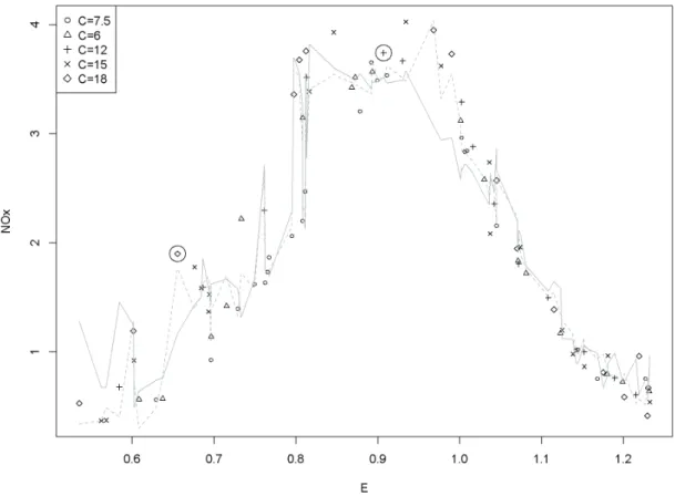
correlation. The shading indicates distances in the predictive means to one recipient P₀px₁“1, x₂“1q. Different draws from the estimated distribution of theβ parameters can alter the definition of the cell from which the donor is drawn. Considering distances, not frequencies, the cell is a circle in the left plot, a long ellipse in the middle plot and a wide ellipse in the right plot. . . 14 4.1 TheNOxdata set by Brinkman (1981) with the optimal local regression fit (q“7, λ“

0, dashed line) and the local regression ﬁt from the grid optimization (q“5, λ“0.2, solid line). . . 23 4.2 The two predictorsC and E of Brinkman (1981) with highlightedP₁ and P₈₈ and

their respectiveq“5 neighborhoods. . . 25 4.3 Regression lines forP₁andP₈₈ . . . 25 D.1 TV consumption on an ordinary day by time of the day and channel . . . 58 D.2 Population boxplot (Rinne, 2008, p. 49) and beeswarm plot (Eklund, 2016) of a

2.5% simple random sample. . . 59 D.3 Convergence plots for the parameter μP8 in one n“600 sample. The dashed line

marks the value of μ_P8 in the population. To better see the dependence on the starting values, the missing values are initially imputed by the column minimum values, which is zero for the variable P8. For the educated procedures the 500 iterations are clearly insuﬃent to get even close to the true value. Ignorant PMM shows very odd behavior beyond the 200th iteration for no obvious reason. The other three ignorant procedures do not show any trend. . . 63 D.4 Plots of the autocorrelation function of the series in ﬁgure D.3 with α“5% con-

ﬁdence intervals. The educated algorithms have a long memory, which is probably caused by the high correlations between the incomplete variables and their trans- formations. Ignorant PMM seems to have a very long memory, too. The other three ignorant procedures have essentially no memory at all. I.e., employing them to sample from the posterior distribution ofμP8 is extremly eﬃcient. . . 64

(8)

D.5 Plots of the autocorrelation function of the series in figure D.3 for the ignorant PMM algorithm. The left plot shows the autocorrelation function based on the entire series with 500 iterations. The right plot is based on the same series, but only on its first 200 data points, i.e., before the odd behavior occurs. The extreme autocorrelation is clearly driven by the odd behavior. However, even disregarding this issue, the values of the autocorrelation function of PMM are much larger than those of the other ignorant algorithms in figure D.4 . . . 64

(9)

List of Tables

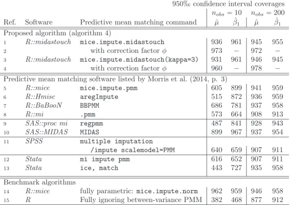
3.1 The algorithms of proper fully parametric imputation, proper approximate Bayesian bootstrap (ABB) imputation, and PMM are compared. The underlying data situation involves two binary predictorspx₁, x₂q, one incomplete variableyh, and normal noise v. The two predictors form Ψ“4 cells: ψpx₁ “0, x₂ “0q “ 1, . . . , ψpx₁ “ 1, x₂ “ 1q “ 4. Ignorability is assumed. In the imputation step, PMM is very similar to ABB imputation, but it ignores the bootstrap. Because ABB imputation is approximately proper, PMM must attenuate the between imputation variance. . 13 3.2 Simulation results. Ref.: reference; 1-8, 14, 15: R Core Team (2016); 5, 14: van

Buuren & Groothuis-Oudshoorn (2011) version 2.22; 6: Harrell (2015); 7: Meinfelder

& Schnapp (2015); 8: Gelman & Hill (2011) version 1.0; 9, 10: SAS Institute Inc.

(2015); 10: Siddique & Harel (2009); 11: IBM Corp. (2015); 12, 13: StataCorp.

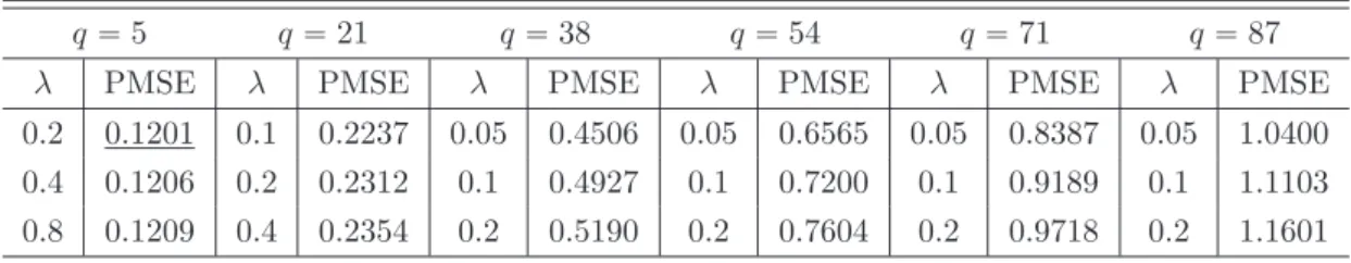
(2015); 13: Royston & White (2011). The results show coverages only, because all algorithms deploy the appropriate linear regression imputation model and diﬀerences in, e.g., biases are not to be expected. . . 18 4.1 Choosing the optimalq and the optimalλ . . . 24 5.1 Simulation results . . . 30 5.2 The table presents relative root mean squared errors (rRMSE)ˆ100. A value of 100

means that the RMSE of the respective parameter estimate in the imputed data set is as large as the RMSE of this parameter before deletion. Coverages of 950inter- vals are given in in parentheses. Abbreviations are: Multiple imputation via local regression (Miles); Predictive mean matching (PMM); Random forest imputation (RF); Passive imputation (PI); Just another variable (JAV).^˚Wheng“0, PMM, PI, and JAV are identical algorithms. ^˚˚The results for JAV and PI in Gaﬀert et al.

(2016) are misleading due to an error in the implementation and are corrected here.

As a consequence, in Gaﬀert et al. (2016) JAV looks worse and PI looks better than it really is. The PI results here are based on 50 Gibbs sampler iterations (see section 2.4). . . 30 6.1 Question on TV consumption in the media survey . . . 35 6.2 Likelihood ratio tests for the MCAR and the MAR assumption. Under the null hy-

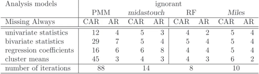
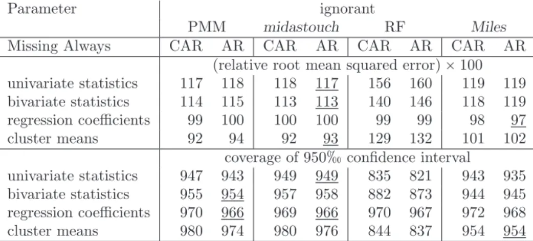
pothesis for the MCAR testprpRq “prpR|Xqholds, and under the null hypothesis for the MAR testprpR|Xq “prpR|Y, Xqholds. . . 36 6.3 First uncorrelated lag as a measure for autocorrelation . . . 39 6.4 Summary of the simulation results. Best in MAAR is underlined. . . 40

(10)

A.1 Characteristics of existing PMM software implementations (Morris et al., 2014, p. 3). The references (Ref.) refer to table 3.2. Abbreviations are: approximate Bayesian bootstrap (ABB), Bayesian bootstrap (BB), in sample (i.s.), and out of

sample (o.o.s). . . 43

A.2 Coverages fornobs“10 split by the three remaining binary factors. The references (Ref.) refer to table 3.2. Abbreviations are: missing always (completely) at random (MA(C)AR). . . 48

A.3 Coverages fornobs“200 split by the three remaining binary factors. The references (Ref.) refer to table 3.2. Abbreviations are: missing always (completely) at random (MA(C)AR). . . 49

D.1 Passively measured data on the TV channels . . . 59

D.2 Basic claims data . . . 60

D.3 Parameters estimates for the response mechanism (N “11916). These estimates are used to delete observations within the simulation study, thereby mimicking natural nonresponse. The estimate for the intercept in the MACAR case of approximately 2 means that it is twice as likely to be observed than to be missing. . . 61

D.4 Contingency tables (N “11916). . . 61

D.5 Regression models (N “11916). . . 62

D.6 Clustering (N “11916). . . 62

D.7 Simulation results: prelative root mean squared errorq ˆ100 . . . 65

D.8 Simulation results: bias relative to the population parameter (in %): 100¨ tř pˆγ´ γqu{pnsims¨γq. . . 66

D.9 Simulation results: coverage of 950conﬁdence intervals. *It is uncertain, whether the clustering fulﬁlls the conditions of Yang & Kim (2016, p. 246), and therefore whether Rubin’s combining rules are appropriate. . . 67

(11)

List of Symbols and Abbreviations

Mathematics: General symbols

Small positive scalar

Ia Identity matrix with dimensionsaˆa fpaq Arbitrary function of a

Btfpaqu{Bpaq First derivative offpaqbya lnpaq Natural logarithm ofa

Random variables and their realizations Q, Y, Z Random variables

prpZq Density function ofZ

yh Incompletenˆ1 vector of realizations of theY variable Yh Realizations of the multivariateY variable (chapter 6 only) i“1, . . . , nobs Index for the observed elements ofy

j “1, . . . , nmis Index for the missing elements ofy

R The random variable indicating the response to the variableY

rh Realizations ofR

Qh Matrix of the completely observed realizations of theQvariables zh Vector of the completely observed realizations of theZ variable

X “ pZ, Qq

Xh Matrix of sizenˆpcomprising a leading constant and the realized pzh, Qhq

x₁ The ﬁrst nonconstant column ofX x₀ The row ofX corresponding to pointP₀

Statistics: General symbols and distributions EpAq Expectation of the random variableA varpAq Variance of the random variableA α Signiﬁcance level for statistical tests i.i.d. Independently identically distributed

A„Npμ, σA²q Afollows a normal distribution with meanμand varianceσ²

Φ Normal distribution function

A„Γ^´1pa₁, a₂q Afollows an inverse-Gamma distribution with parameter a₁ and a₂

A„tpμ, σ², ιq Afollows atdistribution withι degrees of freedom A„χ²pιq Afollows aχ² distribution withιdegrees of freedom N Number of elements in the population

(12)

h“1, . . . , n Index for the sample elements

βˆ Maximum likelihood point estimate of the parameterβ β˜ A draw from the estimated posterior distribution ofβ ωi Vector of bootstrap frequencies of the donors in the sample ρ Pearson’s correlation coeﬃcient

R² Coeﬃcient of determination AIC Akaike information criterion κC Cohen’s kappa (Cohen, 1960)

ψ“1, . . . ,Ψ Number of predictor cells in an analysis of variance (ANOVA) Multiple imputation

m“1, . . . , M Number of multiple imputations

T Total variance of a parameter

W Within variance of a parameter

B Between variance of a parameter

M(C)AR Missing (completely) at random; an assumption about the sample at hand (Rubin, 1976)

The imputation model

β Parameter vector of the imputation model v Residual of the imputation model

σ²_v Variance ofv

ˆ

yh Predicted values from the imputation model based on ˆβ ˆ˜

yh Predicted values from the imputation model based on ˜β The analysis model

γ Parameter vector of the analysis model u Residual of the analysis model

σ²_u Variance ofu

gpQ, Yq Nonlinear function ofpQ, Yq

Predictive mean matching andmidastouch

k Number of respective closest donors in predictive mean matching with drawing probabilities larger zero

ϕ Scalar distance in terms of predicted means between two data points

κ Closeness parameter (Siddique & Belin, 2008)

wj Vector of drawing probabilities of lengthndon for recipientj φ Correction factor for the total variance of the mean under approx-

imate Bayesian bootstrap imputation (Parzen et al., 2005) n_eﬀ Eﬀective sample size (Kish, 1965)

Local regression PMSE Prediction mean squared error: n^´1ř

hpˆyh´yhq² H₀ Neighborhood around the pointP₀

q The number of elements in the neighborhood

(13)

π Order of a polynomial

δ Scalar absolute distance in terms ofXh between two data points d Tricube distance between two data points

C Diagonal weight matrix for weighted least squares regression with d^´1 on the principal diagonal

Λ Diagonal ridge penalty matrix

λ Ridge penalty scalar

l Regression inﬂuence vectors

Simulation studies

rRMSE Root mean squared error of a parameter of interest from the analysis model relative to before deletion

nsim Number of Monte Carlo simulation runs

MA(C)AR Missing always (completely) at random; an assumption about the data generating process (Rubin (1976), Mealli & Rubin (2015))

Imputation algorithms

PMM Predictive mean matching (Rubin (1986), Little (1988))

ABB imputation Approximate Bayesian bootstrap imputation, Rubin & Schenker (1986)

MIDAS Multiple imputation using distance-aided selection of donors (Sid- dique & Belin (2008), Siddique & Harel (2009))

midastouch Touched-up version of MIDAS (chapter 3)

PI Passive imputation (van Buuren & Groothuis-Oudshoorn, 1999) JAV Just-another-variable imputation (von Hippel, 2009)

RF Random forest imputation (Doove et al., 2014) Miles Multiple imputation via local regression (chapter 5)

(14)

Declarations / Erkl¨ arungen

I hereby declare that this dissertation is the result of my own work. It does not include work done by others, particularly not work done by dissertation consultants. Nevertheless, it builds on previously published work that is cited throughout the text and that is fully declared in the bibliography.

Hiermit versichere ich, dass ich die vorliegende Dissertation selbständig und ohne die unzulässige Hilfe Dritter, insbesondere ohne die Hilfe von Promotionsberatern, angefertigt habe. Die aus anderen Quellen direkt oder indirekt bernommenen Gedanken sind im Text als solche kenntlich gemacht und sämtlich im Literaturverzeichnis aufgeführt.

I further state that no substantial part of my dissertation has already been submitted, or, is being concurrently submitted for another degree, diploma or other qualiﬁcation at the Otto- Friedrich-University Bamberg or any other University or similar institution neither in Germany nor abroad.

Hiermit erkläre ich, dass ich keine weiteren Promotionsversuche mit dieser Dissertation oder Teilen daraus unternommen habe. Die Arbeit wurde bislang weder im In- noch im Ausland einer anderen Prüfungsbehörde vorgelegt.

Parts of chapter 3 are published in Teile von Kapitel 3 sind ver¨oﬀentlicht als

Gaﬀert, P., Meinfelder, F. & Bosch, V. (2016). Towards an mi-proper predictive mean matching.

Working Paper. https://www.uni-bamberg.de/fileadmin/uni/fakultaeten/sowi_lehrstuehle/

statistik/Personen/Dateien_Florian/properPMM.pdf, 1-15.

Parts of the chapters 4 and 5 are published in Teile der Kapitel 4 und 5 sind ver¨oﬀentlicht als

Gaﬀert, P., Bosch, V. & Meinfelder, F. (2016). Interactions and Squares: Don’t Transform, Just Impute! In JSM Proceedings, Survey Research Methods Section. Alexandria, VA: American Statistical Association. 2036´2044. Retrieved from http://ww2.amstat.org/sections/srms/

Proceedings/y2016/files/389660.pdf.

(15)

(16)

Chapter 1

Introduction

No institute of science and technology can guarantee discoveries or inventions, and we cannot plan or command a work of genius at will. But do we give sufficient thought to the nurture of the young investigator, to providing the right atmosphere and conditions of work and full opportunity for development? It is these things that foster invention and discovery.

J.R.D. Tata

1.1 Scope

As in other areas of statistics, in data imputation, there are two types of methods, some ad hoc and some model based (Schafer, 1997, p. 1)¹. Among the more sophisticated ad hoc methods is the random hot-deck in adjustment cells (David et al., 1986, p. 30), which will be introduced in more detail in section 2.5.1. A major advantage of this and other hot-deck procedures is that the imputed values are drawn from the empirical distribution of the observed values and are thus plausible (Andridge & Little, 2010, p. 2). The main disadvantage of ad hoc methods is that the underlying assumptions are typically implicit. In contrast, model-based methods explicitly reveal the assumptions that they require. One such model-based method is multiple imputation (Rubin, 1987), which is broadly considered to be ‘simple, elegant and powerful’ (van Buuren, 2012, p.

xix). Multiple imputation is the theoretical framework for the contributions of this dissertation.

However, explicit assumptions are not necessarily more likely to hold in real data. The three most relevant assumptions required for default, i.e., fully parametric, multiple imputation to enable consistent estimation of the parameters of interest are²:

1. Missing at random³: The response rates must not vary systematically after conditioning on

1Calibration weighting is another example. Iterative proportional fitting can be considered an ad hoc method (Deming & Stephan, 1940), and the generalized regression estimator can be considered a model-based method (Cassel et al., 1976).

2This list of three is based on my own experience. Nevertheless, there may be applications in which, e.g., the assumption of independent observations is more doubted than the missing at random assumption.

3Missing at random and distinctness are collectively required forignorability(see section 2.3 and Schafer (1997, p. 10)).

(17)

the observed data, e.g., within adjustment cells, and thus must not depend on the unobserved data (van Buuren, 2012, p. 7).

2. Distribution of the data: In fully parametric multiple imputation, the imputed values are drawn from assumed well-defined distributions, such as the normal distribution (Schafer, 1997, p. 181).

3. Congeniality (Meng, 1994): The imputation model, which is used to predict the missing values of the incomplete variable, must nest all relevant analysis models⁴.

The scope of the dissertation is about relaxing the distributional and the congeniality assumptions to make multiple imputation more attractive to practitioners.

1.2 Outline

Chapters 2 and 4 introduce the theoretical prerequisites for the new ideas in this dissertation.

Chapter 2 places emphasis on multiple imputation (Rubin, 1987), and chapter 4 places emphasis on local regression proposed by Cleveland (1979) and Cleveland & Devlin (1988).

Chapter 3 addresses the required distributional assumption about the data. Predictive mean matching (PMM: Rubin (1986, p. 92), Little (1988, p. 291)), which combines model-based predictions with hot-deck imputations, fully relaxes this assumption. However, PMM is shown to bias multiple imputation variance estimates. Different versions of PMM are introduced, and the new midastouch algorithm, which is based on the ideas of Siddique & Belin (2008), is proposed. A simulation study on multivariate normal data reveals a considerable advantage ofmidastouchover the PMM implementations in the major statistical software packages.

Chapter 5 introduces the newMilesalgorithm. Because it builds onmidastouchfrom chapter 3, Milesdoes not require distributional assumptions. The congeniality assumption, however, cannot be literally relaxed. Rather,Milesfits an imputation model that reflects the major relations, linear or not, between the incomplete variable and its predictors. Analysis models about these major relations are approximately nested in, i.e., congenial to, the (global) imputation model resulting from the local regressions that are employed byMiles. A simulation study on artificial data shows that the approximately congenialMilescan even be superior to fully congenial alternatives.

In the final chapter 6, the newly proposed algorithms are challenged in a simulation study involving real data from the GfK SE company. The evaluations are based on a broad set of analysis models frequently used in market research. Bothmidastouch and Milesperform as well as the established PMM algorithm.

1.3 Contributions

The missing at random assumption

Violating the missing at random assumption can result in seriously biased estimates of the parameters of interest (Enders, 2011, p. 14). However, the practitioner has no indicator for the degree of violation in any specific application (van Buuren, 2012, p. 31). The very special nature of the real data set used in chapter 6 permits a test for the missing at random assumption, which is presented in section 6.2.4. In this setup, the missing at random assumption does not hold. Although this result cannot be generalized, the data set can be used to study the effect of a natural assumption violation in future research.

4or the data generating process (Xie & Meng, 2014, p. 14)

(18)

The distributional assumption

Real data generally do not fit theoretical distributions well. PMM relaxes the distributional assumption. Section 3.2 shows that this relaxation comes at the cost of biasing variance estimates toward zero. While retaining the robust properties of PMM, the newly proposedmidastouch also does not bias variance estimates, as shown in section 3.5.3. Furthermore, when imputing complex missing patterns,midastouch, in contrast to PMM, does not suffer from convergence issues (section 6.3.3).

The congeniality assumption

In slightly nonlinear data,midastouch, although strictly speaking uncongenial, is capable of cap- turing the structure of the data well, and applying Miles does not offer any additional benefit (section 6.4). In the highly nonlinear data of section 5.5.2,Milesperforms better than alternative approximately congenial algorithms and almost as good as the best congenial algorithm, which is the just-another-variable algorithm (von Hippel, 2009) that employs PMM.

Summary

The missing at random assumption remains a serious burden for the imputer, and the contribution of this dissertation to overcome this burden is admittedly quite small.

The newly proposedmidastouchalgorithm fully relaxes the distributional assumption and can also address some congeniality issues, such as in chapter 6, where it is applied to moderately nonlinear data. As an additional benefit, the newly proposed Miles works well even in highly nonlinear data, while being only slightly impaired in perfectly linear data (chapter 5).

In contrast to their competitors random forest imputation (Doove et al., 2014) and PMM, neitherMiles nor midastouch suffer from variance underestimation. Furthermore, in contrast to the just-another-variable algorithm and again PMM, neither midastouch nor Miles suffer from convergence issues when applied to complex missing data patterns. Moreover, in contrast to the just-another-variable algorithm,Milesdoes not cause any consistency issues.

From a practitioner’s perspective, both midastouch and Miles offer considerable robustness compared to the existing alternatives and should be chosen over these alternatives unless there is a specific reason not to do so. Now, ismidastouchbetter thanMilesor vice versa? Milesis superior to midastouch because it can also handle highly nonlinear data. However, Miles is considerably slower thanmidastouch. Our advice is to usemidastouchif time is a concern andMilesotherwise.

1.4 Acknowledgements

I would like to thank Volker Bosch, who came up with the initial idea for this dissertation, which was to use calibration weighting formulas to perform robust data imputation (see section 4.4). It was he who infected me with the curiosity about this topic and who, over the course of the years probably spent months with me developing and rejecting ideas, trying out new things and vividly discussing practical implications. I also want to thank Susanne R¨assler and Florian Meinfelder.

Approximately five years ago, I took their class on multiple imputation at thegesis in Cologne.

Although back then I lacked nearly all the fundamentals, Susi and Flo welcomed me with open arms as their Ph.D. student. Later, Susi, Flo, Volker and I met frequently at thefusion kitchen events and exchanged research ideas. This dissertation would not exist without their inputs.

Susi and Flo have not only introduced me to the field of multiple imputation but also to Stef van Buuren, Donald B. Rubin and Trivellore E. Raghunathan. I would like to thank Raghu for

(19)

diving into the topics of my dissertation so deeply despite joining in rather late in the process. Our discussions made some of my vague ideas turn into precise contributions.

I would like to thank my colleagues at GfK: Markus Lilienthal, Barbara Wolf, and Andreas Kersting for inspiring discussions; Sandra Keller, Christoph Sch¨oll, and Marc Rossbach for their assistance regarding the TV data set in chapter 6; Markus Herrmann for supplying me with the technical infrastructure; Jessica Deuschel, Teodora Vrabcheva, and Erik Hirschfeld for their help with SAS; and Anette Wolfrath, Volker Bosch and Raimund Wildner for supporting my part-time work model.

Most importantly, I would like to thank my wife Veronique. Without her love and support, none of this would have been possible.

(20)

Chapter 2

Multiple Imputation

A capacity, and taste, for reading, gives access to whatever has already been discovered by others. It is the key, or one of the keys, to the already solved

problems. And not only so. It gives a relish, and facility, for successfully pursuing the [yet] unsolved ones.

Abraham Lincoln

2.1 Introduction

Statistical analysis with missing data is no longer a niche problem thanks to the tireless work of, among others, Stef van Buuren and Trivellore Raghunathan, who have not only enhanced the original ideas of Rubin (1978) but also made them accessible to a broad audience through easy to read textbooks (van Buuren (2012), Raghunathan (2015)) and easy to use software (van Buuren

& Groothuis-Oudshoorn (2011), Raghunathan et al. (2002)). Although it is customary to include such a theory chapter in a dissertation (e.g., Siddique (2005), Koller-Meinfelder (2009)), I have, in light of the recent advances, seriously considered dropping this chapter. The only reason for including this chapter is for you, the reader. Therefore, this is not a chapter on general concepts of missing data; rather, it shall filter the parts of the theory that are vital for understanding the new ideas that are presented in the subsequent chapters. In this way, I hope to save the reader some time from looking topics up elsewhere and particularly translating different notations.

2.2 The imputer’s model and the analyst’s model

Statistical analysis is about learning from data. One key element is to apply sensible assumptions.

In the most assumption-free setting, each observation arises from a unique data generating process, and all these processes may be fundamentally different; therefore, it may be completely misleading to link their realizations to any sort of conclusion. Nothing can be learned in this assumption-free setting. Researchers apply assumptions by modeling data. A linear regression model implicitly assumes that the parameters apply to all observations or that the mean effect of an increase of one predictor on the outcome has at least some meaning. Such a model further restricts the relation

(21)

between the predictors and the outcome to be linear in the parameters rather than being arbitrary¹. In the imputation literature, the model that is to be applied to the data, disregarding its com- pleteness, is called the analysis model. The analysis model is derived from the research question.

The purpose of performing imputation is to enable the application of the analysis models of interest, despite facing incomplete data. By ﬁlling the holes in the data set, imputation even relieves the need to adapt the analysis models to the incomplete data situation.

As will be shown in the next section, imputation uses predictive modeling. As long as the imputation model is not more restrictive than the analysis model (Schafer, 1997, p. 141) and the ignorability assumption, which is also described in the next section, is met, the incompleteness does not bias the conclusion of the analysis model². If many different estimands are of interest, i.e., many different analysis models are to be applied to one imputed data set, then the imputation model must be very inclusive at the cost of low efficiency³. The terminclusive is used throughout this dissertation to describe an imputation model that enables at least approximately unbiased estimation of a large number of parameters on the imputed data set and thus in a broader sense than in Collins et al. (2001).

2.3 Parametric multiple imputation

A thorough treatment of multiple imputation and its underlying assumptions is already provided in Rubin (1987) and discussed in detail in Schafer (1997). This section consists of a less general example that will be revisited in the next chapter.

Let the data of interest benindependent realizations of a normal random vectorpQ, Y, Zqwith lengthp. Throughout this dissertation,Qwith lengthp´2 denotes one or more predictors in both the imputation model and the analysis model. Y denotes the variable with missing values and thus the response variable in the imputation model, andZ denotes the response variable in the analysis model. The matrix of independentpZ, Qqrealizations Xh with dimensions nˆpis fully observed and is deﬁned to include a leading constant column. The realization r of the random vectorRtakes the value 1 for allnobs observed values ofyh and 0 for allnmis “n´nobsmissing values ofyh. The imputation model is the linear model

yh“Xhβ`v with v„Np0, σ²vInq, (2.1) whereβ denotes a vector of parameters of lengthp. In fully parametric multiple imputation, the steps of algorithm 1 are repeatedM ě2 times to correctly reﬂect the uncertainty of the parameter estimates of the imputation model.

The key assumption required for this procedure is that the missing values are not governed by a different regime than the observed values. This assumption means that the imputation model in equation (2.1) is not misspecified even though it does not involver, or, more formally, thatrandv must be independent. This requirement is known as the missing at random (MAR) assumption⁴. A stricter version is the missing completely at random (MCAR) assumption, which implies thatr andy must be independent. Ifrandv are somehow related, then the response mechanism is said to be missing not at random (MNAR). Similar relations can be defined for the data generating process, resulting in the terms missing always at random (MAAR) and missing always completely

1The list of necessary assumptions for the linear regression model is even much longer (Greene, 2008, p. 44).

2An unusual exception to this rule is supereﬃciency (Rubin, 1996, p. 481).

3In these cases it may be beneﬁcial to use diﬀerent imputation models, e.g., one for each analysis model.

4Strictly speaking, missing at random and an additional, rather minor, assumption, called distinctness (Schafer, 1997, p. 11), are required for the response mechanism to beignorable.

(22)

Algorithm 1 Parametric multiple imputation for a single normal incomplete variableyh and a set of complete linear predictorsXh (Little & Rubin (2002, p. 216), Greenberg (2013, p. 116)).

The steps are named according to Tanner & Wong (1987, p. 531) although this algorithm is not iterative.

1. The posterior step to draw the parameters: First, draw from the observed data posterior distribution of the residual variance, which is prp˜σ²_v|yi, Xiq “Γ^´1tnobs{2,pyi´Xiβqˆ ¹pyi´ Xiβˆq{2u (Greene, 2008, p. 996). Then, draw from the observed data posterior distribution of the intercept and slope parameters, which is prpβ˜ |yi, Xi,σ˜²_vq “Nptβ,ˆ σ˜²_vpXi¹Xiq^´1u. yi

andXi refer to the fully observed subset of the data, and ˆβdenotes the maximum likelihood parameter estimate (Greene, 2008, p. 483).

2. The imputation step to draw the missing values conditional on the parameters: Drawnmis

times independently from the imputation model, i.e., ˜yj „NpXjβ,˜ σ˜²_vqwithj“1, . . . , nmis.

at random (MACAR) (Rubin (1976), Mealli & Rubin (2015)). The work in this dissertation does not involve MNAR. Useful practical implications of the MAR assumption are derived in van Buuren (2012, p. 34).

The analysis model shall now be applied to each imputed data set. Suppose that the estimand is the mean of Y. The M diﬀerent maximum likelihood estimates pˆμ^m_y^“1, . . . ,μˆ^m_y^“^Mq can be combined using Rubin’s rules (Rubin, 1987, p. 76) by ˆμy“M^´1řM

m“1μˆ^m_y . The variance is given by

T “varpμˆyq “M^´1pn´1q^´1 ÿM m“1

tvarpy_h^mqu loooooooooooooooooomoooooooooooooooooon

W

`p1`M^´1q pM ´1q^´1 ÿM m“1

pμˆ^m_y ´μˆyq² loooooooooooooooomoooooooooooooooon

B

(2.2)

Equation (2.2) involves an analysis of variance (ANOVA) type thinking (Rinne, 2008, p. 650). The withinvarianceW is the variance as in a completely observed data set, and thebetween varianceB reﬂects the uncertainty that is involved in estimating the imputation model parametersβ andσ_v². If the imputation model had no parameters to estimate, e.g.,yh“2zh, then the between variance would be zero. However, note that suchrestrictive imputation models typically do not nest any relevant analysis models and thus bias their conclusions (see section 2.2). The quantityT^´0^.⁵μˆy

istpμ,1, ιqdistributed (Rinne, 2008, p. 326) with degrees of freedom (Barnard & Rubin, 1999, p.

949)

ι“

«

pM ´1q^´1 ˆ

1` M

M`1 W

B

˙_´2

` n`2 npn´1q

T W

ﬀ_´1 .

Rubin (1987, p. 118) calls imputations that yield approximately valid inferences for the parameters of interestproper. The detailed requirements are presented in (Schafer, 1997, p. 145).

2.4 Missing data patterns

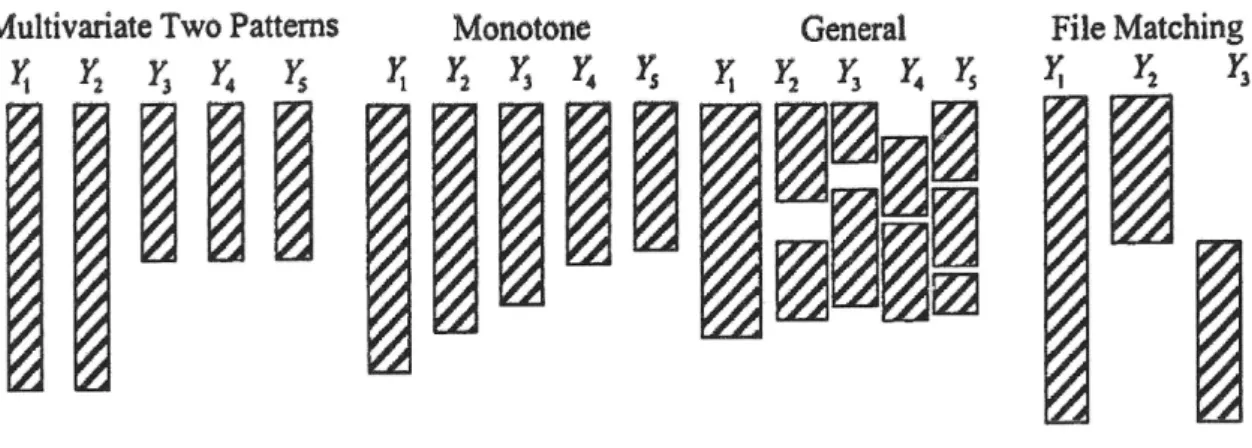
The example in the previous section consists of only one incomplete variable. In real data applications, two or more variables are generally incomplete. We distinguish three diﬀerent cases, which are also shown in ﬁgure 2.1.

1. Monotone pattern and multivariate two patterns. An appropriate algorithm proceeds as follows. Imputations are drawn from the imputation model, such as the one in equation 2.1 for the ﬁrst incomplete variable conditional on all fully observed variables. The imputations for the second variable are drawn conditional on all fully observed variables and the ﬁrst

(23)

Figure 2.1: Relevant missing patterns for this text (Little & Rubin, 2002, p. 5)).

imputed variable, and so on. The last variable in the data set is imputed conditional on all variables but itself (van Buuren, 2012, p. 104). The multivariate two patterns are a special case of the monotone pattern and will be revisited in chapter 5.

2. Swiss cheese (Andridge, 2011, p. 67) a.k.a. general pattern. An appropriate algorithm starts with a simple random hot-deck, i.e., with drawing randomly from the observed values within each variable (van Buuren & Groothuis-Oudshoorn, 2011, p. 18), and iterates over the variables. There are two differences to the algorithm for the monotone pattern: conditioning is always on all other variables, and the algorithm does not stop when the end of the data set is reached. Rather, the algorithm iterates over all variables in the data set as often as required to reach convergence for the parameters of the analysis model. Kennickell (1991) was the first to apply this sequential regression algorithm, which is akin to Gibbs sampling and often referred to as fully conditional specification or chained equations (van Buuren &

Groothuis-Oudshoorn, 2011). For a thorough treatment, see Raghunathan et al. (2001) and Liu et al. (2013). The Swiss cheese pattern will be revisited in chapter 6.

3. File matching pattern. In the file matching pattern, the complete cases maximum likelihood estimate of the parameter of interest is unobtainable. The typical example is a correlation co- efficient of two variables that are never jointly observed. Although the file matching pattern, which is also known as data fusion, is very relevant in market research, it is not covered in this dissertation. For a thorough treatment, see Raessler (2002) and D’Orazio et al. (2006).

2.5 Alternatives to fully parametric algorithms

2.5.1 Hot-deck imputation

As shown in algorithm 1, in fully parametric imputation, the values are drawn from well-described distributions, which hardly fit empirical distributions. A simple solution is to impute observed values from the same variable, i.e., to provide the ‘recipients’ values from the ‘donors’. The obvious advantage of these hot-deck procedures is that the imputed values are plausible and do not, e.g., fall outside the range. The simple random hot-deck has already been introduced above.

Valid descriptive statistics can be obtained from a simple random hot-deck imputation if there is only one variable and the response mechanism is completely at random. However, unlessnobs is very large, confidence intervals are excessively short because the between variance component B

(24)

of equation (2.2) is ignored. The simple random hot-deck omits the posterior step (Siddique, 2005, p. 17).

A natural extension of the simple random hot-deck evolves from the presence of categorical predictors. The simple random hot-deck can then be performed within each cell, which is similar to ﬁtting an ANOVA model containing all interactions (Lillard et al., 1982, p. 15). The imputed value can be regarded as the cell mean plus the residual of the randomly selected donor.

2.5.2 The approximate Bayesian bootstrap

Bayesian bootstrap imputation resolves the inference issue of simple random hot-deck. The absolute frequencies of the observed values serve as the parameters of a Dirichlet distribution (Rinne, 2008, p. 350). The underlying assumption is that the variable is categorical with as many categories as there are unique values. Draws from this distribution deﬁne the parameters of multinomial distributions (Rinne, 2008, p. 277). Draws from the multinomial distributions in turn yield the multiple imputations. Rubin & Schenker (1986, p. 368) provide the details.

The approximate Bayesian bootstrap imputation can be regarded as a computational shortcut of the Bayesian bootstrap imputation. In the posterior step, a bootstrap sample from the donors is drawn (Efron, 1979), and the imputations are simply drawn from this bootstrap sample (Rubin

& Schenker, 1986, p. 368). This implicit modeling procedure propagates the uncertainty of the estimated parameters involved. However, Kim (2002) shows that the conﬁdence intervals are still too small because, just like the maximum likelihood estimator, the bootstrap estimator ignores the correction for the appropriate number of degrees of freedom (Davison & Hinkley, 1997, p. 22).

Therefore, for ﬁnitenobs, the total parameter variance is still slightly underestimated. Parzen et al.

(2005) show that multiplying the total variance estimator for the mean presented in equation (2.2) by the following factorφeliminates this bias

φpnobs, nmis, Mq “

n²

n_obs `ⁿ^misM

´n´1 n_obs´_nⁿ2

obs

¯

n2

n_obs `ⁿ^misM

´n´1 n_obs´_nⁿ2

obs

¯´ⁿn^¨ⁿ_obs^mis

´3 n `n_obs¹

¯ ě1. (2.3)

Some criticism regarding this correction factor has been presented by Demirtas et al. (2007).

2.5.3 Predictive mean matching (PMM)

In contrast to the approximate Bayesian bootstrap, in PMM (Rubin, 1986, p. 92), only the imputation step of algorithm 1 is modiﬁed. The ﬁrst implementation of PMM for general missing data problems by Little (1988) is still widely used (e.g., van Buuren & Groothuis-Oudshoorn (2011), Royston & White (2011)⁵) and is thus the key reference (see algorithm 2).

Algorithm 2The original PMM algorithm proposed by Little (1988, p. 292).

1. Calculate the predictive mean for thenobsobserved elements ofyh as ˆyi“Xiβ.ˆ 2. Calculate the predictive mean for thenmis missing elements ofyhas ˆy˜j “Xjβ.˜ 3. Match each element of ˆy˜j to its corresponding closest element of ˆyi.

4. Impute the observedyi of the closest matches.

5Both implementations deviate from the original algorithm in that they make a random draw from the closest ką1 donors in the last step.

(25)

Compared to fully parametric imputation, PMM is more robust to model misspeciﬁcations (Schenker & Taylor, 1996, p. 429), namely, nonlinear associations, heteroscedastic residuals, and deviations from normality (Morris et al., 2014, p. 4). Nonetheless, the quality of PMM imputations largely depends on the availability of nearby donors; truncation of the data limits the validity of the method (Koller-Meinfelder, 2009, p. 38).

While retaining the benefits of the simple random hot-deck in cells discussed above, PMM has additional desirable properties. The most obvious such property is a more flexible imputation model, which neither requires the continuous predictors to be divided into arbitrary categories nor needs all interactions to be considered. Because the matching is not affected by variables that are not predictive, PMM can also be considered more parsimonious (David et al., 1986, p. 31).

2.5.4 Distance-aided donor selection

For the posterior step of the distance-aided donor selection algorithm proposed by Siddique (2005) and Siddique & Belin (2008), which Siddique & Harel (2009) later called MIDAS, bootstrapping is employed as originally proposed by Heitjan & Little (1991, p. 18). Maximum likelihood estimation of the linear regression imputation model parameters onM independent bootstrap samples replaces the draws from the posterior distribution (Little & Rubin, 2002, p. 216). The unique feature of the MIDAS algorithm is that it reuses the donors’ bootstrap frequencies for the imputation step.

For recipientj, donoriis drawn from the full donor pool with probability wi,j“fpω,yˆ˜i,yˆ˜j, κq “ωiϕˆ˜^´_i,j^κ{

nÿ_obs

i“1

pωiϕˆ˜^´_i,j^κq, (2.4)

where ωi denotes the bootstrap frequency of donor i, ˆϕ˜i,j denotes the scalar absolute distance between the predictive means of donoriand recipientjbased on ˜β, andκis a closeness parameter that adjusts the importance of the distance. For κ“ 0, the procedure is equivalent to the approximate Bayesian bootstrap; forκÑ 8, the procedure becomes equivalent to nearest-neighbor matching, as in algorithm 2.

2.5.5 Random forest imputation

The choice of any model is a bias-variance trade-off. If the analysis model is known, then all parameters that are not of interest may be biased by the imputation model without any additional harm. However, if the analysis model is unknown, then it is the imputer’s job to find an imputation model that neither restricts the key relations in the data nor suffers from low efficiency.

Incorporating, for instance, interactions in parametric imputation models becomes ineﬃcient very quickly because the number of parameters to estimate increases quadratically with the number of variables.

Doove et al. (2014) suggest using random forest imputation to implicitly include non-linear relations. They show that their algorithm preserves interactions that are not explicitly contained in the imputation model quite well and substantially better than posterior-step linear regression models with imputation-step PMM. This improvement, however, comes at the cost of biasing the linear eﬀects of regression analysis models (Doove et al., 2014, p. 101).

For their implementation Doove et al. (2014) use the R::mice framework for sequential regressions (van Buuren & Groothuis-Oudshoorn, 2011) and theR::randomForestpackage (Liaw &

Wiener, 2002), which consists of ﬁtting classiﬁcation and regression trees. A thorough theoretical treatment thereof is provided in James et al. (2013, p. 303) and the implementation is presented

(26)

Algorithm 3The random forest imputation algorithm by Doove et al. (2014, p. 103).

1. Drawntree bootstrap samples from the donors.

2. Drawntree random samples of sizepp´1q{3 from thep´1 predictor variables.

3. Fitntreetrees by recursive partitioning without pruning^˚. Each leaf of each tree constitutes a subset of the donors.

4. Put the recipients down the trees to see in which leaves they fall.

5. Combine all leaves including the same recipient over all trees to one donor poolDj for each recipientj.

6. For each recipientj make a random draw fromDj and impute the value of the drawn donor.

˚The term pruning encompasses diﬀerent algorithms that reduce the complexity of the tree to avoid overﬁtting.

in algorithm 3.

2.5.6 Others

There are a few other algorithms that promise to address nonlinear data. Similar to random forest imputation, the latent-class based algorithm by Akande et al. (2016) forms groups of donors and recipients such that the imputations are obtained by simply drawing donors from the same group.

TheR::Hmisc::aregImputealgorithm by Harrell (2015) (R Core Team, 2016), which is based on the theoretical work by Breiman & Friedman (1985), results in predictions of transformedyh and employs PMM in the imputation step. Neither of the two algorithms is within the scope of the next chapters.

(27)

Chapter 3

Toward

Multiple-Imputation-Proper Predictive Mean Matching

It is by intuition that we discover and by logic we prove.

Henri Poincar´e

3.1 Introduction

Combining multiple imputation with predictive mean matching (PMM) promises to provide a robust imputation procedure that will yield valid inferences, thus making it highly appealing to practitioners (Heitjan & Little, 1991, p. 19). Consequently, such a combination is not only a feature but also often the default mode of imputation algorithms in all major statistical software programs (Morris et al., 2014, p. 3). Despite its preeminence in practice, skepticism regarding this combination of techniques dominates the literature. Little & Rubin (2002, p. 69) state the following about PMM

... properties of estimates derived from such matching procedures remain largely unexplored.

Koller-Meinfelder (2009, p. 32) notes that

The difficult part about Predictive Mean Matching is to utilize its robust properties within the Multiple Imputation framework in a way that Rubin’s combination rules still yield unbiased variance estimates.

Moreover, Morris et al. (2014, p. 5) recently warned in the same context

... there is thus no guarantee that Rubin’s rules will be appropriate for inference.

The contrast between the theoretical uncertainty concerning the validity of this combined approach and its popularity in applications motivated the work presented in this chapter. The next section elaborates one major deviation of multiple imputation PMM algorithms from the theory of multiple imputation, which is one of the key contributions of this dissertation. The new insight sheds a

(28)

different light on well-known tuning parameters for PMM, which are presented in section 3.3. A new and more proper algorithm is proposed in section 3.4, whose empirical superiority regarding the coverages of frequentist confidence intervals is demonstrated via a simulation study in section 3.5. The insights of this chapter are published as a working paper (Gaffert et al., 2016), and citing it is spared throughout.

3.2 Why predictive mean matching is not multiple imputa- tion proper

Using PMM for the multiple imputation of data sets causes the between variance of the parameter estimates of interest to suﬀer from attenuation bias.

To illustrate this situation, consider an analysis of variance example withψ“1, . . . ,Ψ different predictor cells. Suppose that the incomplete variableY in cellψis normally distributed with mean μψand varianceσ²_ψ. Furthermore, suppose that each of the Ψ cells contains a sufficient number of donors, say, five or more. Now, without loss of generality, let us examine at the recipients in the first cell. Parametric multiple imputation drawsM ě2 times ˜σ₁², then ˜μ₁|σ˜₁², and then ˜yψ“1| pμ˜₁,σ˜₁²q, which is efficient. A nonparametric alternative is an approximate Bayesian bootstrap imputation in cell ψ “ 1 that proceeds as follows. It draws M ě 2 times a bootstrap sample from the donors in the cell and draws values to impute from this bootstrap sample. The key element that these two proper procedures have in common is that the distribution from which the imputed values are drawn varies over the multiple imputations. In the parametric case the parameters of the underlying normal distributions vary, and in the nonparametric case, the composition of the empirical distribution varies.

fully parametric PMM ABB imputation

Posterior step Drawpβ,˜ σ˜_v²qfrom the imputation modelyh“ β₀ `β₁x₁ `β₂x₂ `β₃x₁x₂ `v, with het- eroscedastic residuals, i.e., varpv |ψ “1q “ σ²_v,₁,. . .,varpv|ψ“4q “σ²_v,₄.

Within each of the Ψ “ 4 cells draw a bootstrap sample of the nobs,1, . . ., nobs,4 donors

Imputation step Draw from the normal imputation model: ˜yj | pβ,˜ σ˜²_v, x₁, x₂q

As within each cell the predicted means ˆy˜ψ are identical, algorithm 2 drawsnmis,ψ

values from nobs,ψ, i.e., a simple random hot-deck imputation within the cell

Within each cell, draw nmis,ψ values from the bootstrapped nobs,ψ, i.e., a simple random hot- deck imputation within thebootstrapped cell Table 3.1: The algorithms of proper fully parametric imputation, proper approximate Bayesian bootstrap (ABB) imputation, and PMM are compared. The underlying data situation involves two binary predictorspx₁, x₂q, one incomplete variableyh, and normal noisev. The two predictors form Ψ “ 4 cells: ψpx₁ “0, x₂ “ 0q “ 1, . . . , ψpx₁ “ 1, x₂ “ 1q “4. Ignorability is assumed.

In the imputation step, PMM is very similar to ABB imputation, but it ignores the bootstrap.

Because ABB imputation is approximately proper, PMM must attenuate the between imputation variance.

PMM proceeds in a considerably diﬀerent manner. The recipients and the donors in cellψ“1 end up having exactly the same predicted mean¹. Choosing the nearest neighbor ultimately consists of making a random draw from the donors in cellψ“1. This may be valid once, but the procedure is the same for all m“1, . . . , M imputations. It thereby mimics the simple random hot-deck of

1This is only true if type-2 matching is applied, which slightly diﬀers from algorithm 2. Section 3.3 presents the details.

(29)

section 2.5.1, which is known to underestimate the between variance component because it partly omits the posterior step. Table 3.1 schematically presents this reasoning.

It appears to be surprising that although PMM contains a draw from the estimated distribution of the intercept and slope parameters β (see algorithm 2), the parameter uncertainty does not propagate. In this regard, the above example is deceptive. Therefore, consider another example.

For simplicity, suppose that there are two normal orthogonal predictorsx₁, x₂. Now, the definition of the relevant donors is less clear than in the previous example, where it appeared obvious that all donors ofψ“1 are suitable. The job of theβ is simply to define the relevant ‘cell’. Drawing ˜β is an important task, because the cell definition is not certain and must thus vary over the multiple imputations. Figure 3.1 displays the effect of varyingβ coefficients on the cell definition.

Figure 3.1: The plots show 100 random draws from a bivariate normal distribution with zero correlation. The shading indicates distances in the predictive means to one recipient P₀px₁ “ 1, x₂ “ 1q. Diﬀerent draws from the estimated distribution of the β parameters can alter the deﬁnition of the cell from which the donor is drawn. Considering distances, not frequencies, the cell is a circle in the left plot, a long ellipse in the middle plot and a wide ellipse in the right plot.

However, PMM then goes wrong. The cells are defined, i.e., we have conditioned on ˜β, and all PMM does is make a random draw from the cell or even take the nearest one. It thereby ignores parameter uncertainty to a large extent. To be precise, the ˜β define the mean of the cell; however, the uncertainty in estimating the residual variance parameter σ²_v from the imputation model in equation (2.1) remains unconsidered. In any given cell, we observe a distribution of units in a sample, which suffers from sampling error. Thus, what is needed is some type of approximate Bayesian bootstrap imputation algorithmafter conditioning on the ˜β parameters.

3.3 Existing ideas to make predictive mean matching proper

PMM has recently been under suspicion for underestimating the between variance component of equation (2.2). Van Buuren (2012, p. 71) and Morris et al. (2014, p. 7) criticize the selection of the nearest neighbor of algorithm 2. Selecting the nearest neighbor is a special case of general k-nearest-neighbor selection (Heitjan & Little, 1991, p. 16), which is typically applied in current statistical software programs (see table A.1). An adaptive procedure for choosing the optimal k exists (Schenker & Taylor, 1996, p. 442), but software implementations of this procedure are lacking. The attenuation bias argument is thatk“1 leads to selecting the same donor repeatedly across imputations. The insight of section 3.2 is that once the cell is deﬁned, the bootstrap