The application of nonparametric data augmentation and imputation using classiﬁcation and regression trees within a large-scale panel study

(1)

The application of nonparametric data augmentation and imputation using classification and regression trees within a

large-scale panel study

Dissertation

Presented to the Faculty for Social Sciences, Economics, and Business Administration at the University of Bamberg in Partial Fulfillment of the Requirements for the Degree of

DOCTOR RERUM POLITICARUM by

Dipl.-Pol. Solange Diana Goßmann, born July 23, 1985 in Buenos Aires, Argentina

Date of Submission

March 29, 2016

(2)

II

Principal advisor: Prof. Dr. Susanne R¨assler University of Bamberg, Germany Reviewers: Prof. Dr. Kai Fischbach

University of Bamberg, Germany Prof. Dr. Guido Heineck

University of Bamberg, Germany Date of Submission: March 29, 2016

Date of defence: November 07, 2017

URN: urn:nbn:de:bvb:473-opus4-509982 DOI: https://doi.org/10.20378/irbo-50998

(3)

III

Abstract

Generally, multiple imputation is the recommended method for handling item nonresponse in surveys. Usually it is applied as chained equations approach based on parametric models. As Burgette & Reiter (2010) have shown classification and regression trees (CART) are a good alternative replacing the parametric models as conditional models especially when complex models occur, interac- tions and nonlinear models have to be handled and the amount of variables is very large. In large-scale panel studies many types of data sets with special data situations have to be handled. Based on the study of Burgette & Reiter (2010), this thesis intends to further assess the suitability of CART in combination with multiple imputation and data augmentation on some of these special situations.

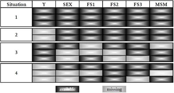
Unit nonresponse, panel attrition in particular, is a problem with high impact on survey quality in social sciences. The first application aims at imputing missing values by CART to generate a proper data base for the decision whether weighting has to be considered. This decision was based on auxiliary information about respondents and nonrespondents. Both, auxiliary information and the participation status as response indicator, contained missing values that had to be imputed. The described situation originated in a school survey. The schools were asked to transmit auxiliary information about their students without knowing if they participated in the survey or not. In the end both information, auxiliary information and the participation status, should have been combined by their identification number by the survey research institute. Some data were collected and transmitted correctly, some were not. Due to those errors four data situations were distinguished and handled in different ways. 1) Complete cases, that is no missing values neither for the participation status, nor the auxiliary information. That means that the information whether the student participated were available and the auxiliary information were completely observed and correctly merged. 2) The participation status was missing, but the auxiliary information were complete. That happened when the school transmitted the auxiliary data of a student completely, but the combination with the survey participation information failed. 3) The participation status was available, but there were missings

(4)

IV

in the auxiliary information and 4) there were missings in participation status as well as in the auxiliary information.

The procedure to handle the complete data situation 1) was a standard probit analysis. A Probit Forecast Draw was applied in situations 2) and 4) which was based on a Metropolis-Hasting algorithm that used the available information of the maximum number of participants conditional on an auxiliary variable. In practice, the amount of male and female students that participated in the survey was known. This number was used as a maximum when the auxiliary information were combined with a probable participation status. All missings in auxiliary information, that was situations 3) and 4), were augmented by CART. That means that the imputation values were drawn via Bayesian Bootstrap from final nodes of the classification and regression trees. Both, the imputation and the probit model with the response indicator as the dependent variable resulted in a data augmentation approach. All steps were chained to use as much information as possible for the analysis.

The application shows that CART can flexibly be combined with data augmentation resulting in a Markov chain Monte Carlo method or more precisely a Gibbs sampler. The results of the analysis of the (meta-)data showed a selectivity due to nonparticipation which could be explained by the variable sex. Female students tended to participate more likely than male students. The results based on the usage of CART differed clearly from those of the complete cases analysis ignoring the second level random effect as well as from those outcomes of the complete cases analysis including the second level random effect.

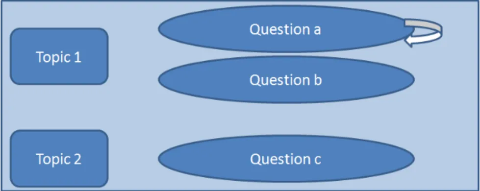
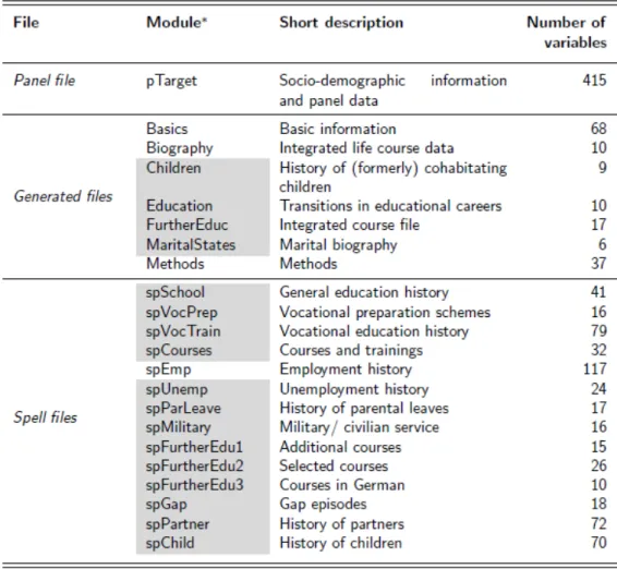
Surveys based on flexible filtering offer the opportunity to adjust the questionnaire to the respondents’ situation. Hence, data quality can be increased and response burden can be decreased. Therefore, filters are often implemented in large-scale surveys resulting in a complex data structure, that has to be considered when imputing. The second study of this thesis shows how a data set containing many filters and a high filter-depth that limits the admissible range of values for multiple imputation can be handled by using CART. To get more into detail, a very large and complex data set contained variables that were used for the analysis of household net income. The variables were distributed over modules. Modules

(5)

V

are blocks of questions reffering to certain topics which are partially steered by filters. Additionally, within those modules the survey was steered by filter questions. As a consequence the number of respondents on each variable differed.

It can be assumed that due to the structure of the survey missing values were mainly produced by filters or caused by the respondent intentionally and only a minor part were missing e.g. by interviewers overseeing them.

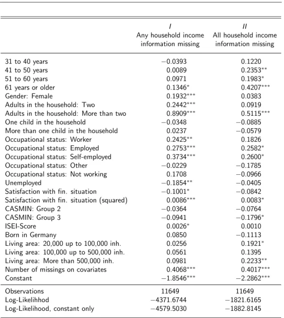
The second application shows that the described procedure is able to consider the complex data structure as the draws from CART are flexibly limited due to the changing filter structure which is generated by imputed filter steering values as well. Regarding the amount of 213 chosen variables for the household net income imputation, CART in contrast to other approaches obviously leads to time sav- ings as no model specification is needed for each variable that has to be imputed.

Still, there is a need to get some feedback concerning the suitability of CART- based imputation. Therefore, as third application of this thesis, a simulation study was conducted to show the performance of CART in a combination with multiple imputation by chained equations (MICE) on cross-sectional data. Addi- tionally, it was checked whether a change of settings improves the performance for the given data. There were three different data generating functions of Y. The first was a typical linear model with a normally distributed error term. The second included a chi-squared error term. The third included a non-linear (loga- rithmic) term. The rate of missing values was set to 60% steered by a missing at random mechanism. Regression parameters, mean, quantiles and correlations were calculated and combined. The quality of the estimation for before deletion, complete cases and the imputed data was measured by coverage, i.e. the proportion of 95%-confidence intervals for the estimated parameters that contain the true value. Additionally, bias and mean squared error were calculated.

Then, the settings were changed for the first type of data set, that was the ordinary linear model. First, the initialization was changed to a tree-based initialization instead of draws from the unconditional empirical distribution. Second, the iterations of the tree-based MI approach were increased from 20 to 50. Third, the number of imputed data sets that were combined for the confidence intervals was doubled from 15 to 30. CART-based MICE showed a good performance

(6)

VI

(88.8% to 91.8%) for all three data sets. Additionally, it was not worthwhile changing the settings of CART for the partitioning of the simulated data.

Moreover, the third application shows some insights about the performance and the settings of CART-based MICE. There were many default settings and pecu- liarities that had to be considered when using CART-based MICE. The results suggest that the default settings and the performance of CART in general lead to sufficient results when conducted on cross-sectional data. Respective the settings, changing the initialization from tree-based draws to draws from the un- conditonal empirical distribution is recommendable for typical survey data, that is data with missing values in large parts of the data.

The fourth application gives some insights into the performance of CART-based MICE on panel data. Therefore, the first simulated data set was extended to panel data containing information from two waves. Four data situations were distinguished, that was three random effects models with different combinations of time-variant and time-invariant variables and a fixed effects model. The last was defined by an intercept that is correlated to a regressor, the missingness steering variable X₁. CART-based MICE showed a good performance (89.0% to 91.4%) for all four data sets. CART chose the variables from the correct wave for each of the four data situations and waves. That means that only first wave information was used for the imputation of the first wave variableY_t=1, respec- tively only second wave information was used for the second wave variable Y_t=2. This is crucial as the data generation for each of both waves was conducted as either independent of the other wave or the variables were time-variant for all four data situations.

This thesis demonstrates that CART can be used as a highly flexible imputation component which can be recommended with constraints for large-scale panel studies. Missing values in cross-sectional data as well as panel data can both be handled with CART-based MICE. Of course, the accuracy depends on the availability of explanatory power and correlations for both, cross-sectional and panel data. The combination of CART with data augmentation and the exten- sion concering the filtering of the data are both feasible and promising.

(7)

VII

In addition, further research about the performance of CART is highly recommended, for example by extending the current simulation study by changes of the variables over time based on past values of the same variable, more waves or different data generation processes.

Keywords: missing data, multiple imputation by chained equations, data augmentation, classification and regression trees

(8)

VIII

Basis for this thesis

This thesis is partly based on the following publications which are joined work with other authors:

Aßmann et al. (2014a)

Aßmann et al. (2014b)

Aßmann et al. (2015)

However, the thesis focuses on my contribution to those publications and only refers to the joint work when it is crucial for a better understanding.

The data in chapter 3 differ from the scientific use file ’Organizational Re- form Study in Thuringia (TH)’ data from the National Educational Panel Study (NEPS) as it includes sensitive data which are only available for intern staff.

The scientific use file is available at http://dx.doi.org/10.5157/NEPS:TH:

1.0.0. In chapter 4 data from the NEPS are used as well: Starting Cohort 6 - Adults (Adult Education and Lifelong Learning), doi:10.5157/NEPS: SC6:1.0.0.

From 2008 to 2013, NEPS data were collected as part of the Framework Program for the Promotion of Empirical Educational Research funded by the German Fed- eral Ministry of Education and Research (BMBF). As of 2014, NEPS is carried out by the Leibniz Institute for Educational Trajectories (LIfBi) at the University of Bamberg in cooperation with a nationwide network. More information about the NEPS can be found in Blossfeld et al. (2011).

The software used is R, see R Core Team (2014).

The approach of Burgette & Reiter (2010) which gave the impulse to this thesis is provided asR-Syntax athttp://www.burgette.org/software.html. New is an implementation of CART within theMICE-package usingmice.impute.cart which was not used for this thesis as it was not available when the process started and continued.

(9)

Declaration of academic honesty

I hereby confirm that my thesis is the result of my own work. I did not recieve any help or support from commercial consultants. All sources or materials applied are listed and specified in the thesis. I have explicitly marked all material which has been quoted either literally or by content from the used sources.

Furthermore, I confirm that this thesis has not yet been submitted as part of another examination process neither in identical nor in similar form.

Solange Goßmann

Bamberg, March 29, 2016

(10)

X

(11)

List of Figures

2.1 Matrices Y and R indicating observed and missing values . . . 8

2.2 Example of a regression tree . . . 19

3.1 Data with auxiliary variables . . . 27

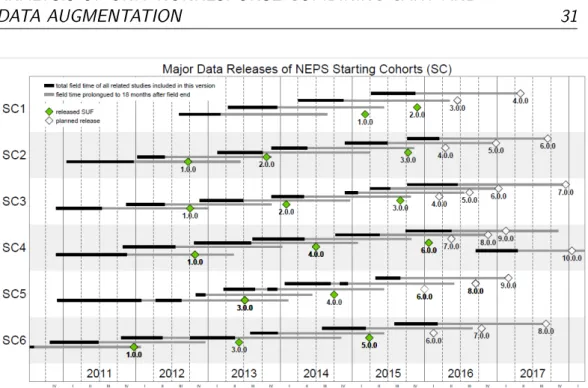
3.2 NEPS Data Releases, available from https://www.neps-data .de/en-us/datacenter/overviewandassistance/releaseschedule .aspx (Date of download: 22.02.2016) . . . 31

3.3 Missingness pattern of the Thuringia study data . . . 34

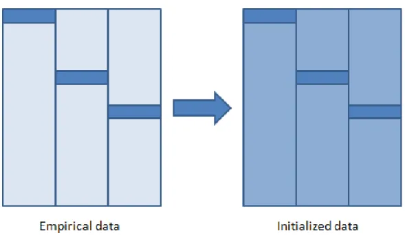
3.4 Empirical and initialized data . . . 41

4.1 Pathway through a survey with questions arranged by topic . . . 45

4.2 Filter type 1, only affecting the same variable . . . 46

4.3 Filter type 2, affecting a variable of the same topic . . . 47

4.4 Filter type 3, affecting a variable of another topic . . . 47

4.5 Filter type 4, affecting a whole topic module . . . 48

4.6 Unchained filters influencing one variable . . . 50

4.7 Chained filters influencing one variable . . . 50

4.8 Imputation of missing values when there is a filter hierarchy to be regarded . . . 51

4.9 Modules in the NEPS SUF SC6 . . . 54

5.1 Results from the analysis of Koller-Meinfelder (2009) . . . 74

6.1 Data in longformat and wideformat . . . 86 XV

(16)

XVI LIST OF FIGURES

6.2 Resulting tree of one imputation cycle for the imputation of Y_t=1 of DS1. Notes: the mean is always with reference to Y_t=1, N is the number of respondents in each node, the split points are rounded to two decimals for better display. . . 97 6.3 Resulting tree of one imputation cycle for the imputation of Yt=2

of DS1. Notes: the mean is always with reference to Y_t=2, N is the number of respondents in each node, the split points are rounded to two decimals for better display. . . 98 B.1 Draws from the Gibbs sampler . . . 126 B.2 Plots of the autocorrelation functions (ACF) . . . 127 B.3 Income questions in the NEPS SUF SC6 – exact estimate and

two-stage income brackets. . . 128 B.4 Household net income imputed via the main panel file and two

generated files. Notes: mean is always with reference to household income, N is the number of respondents in each node. . . . 129 B.5 Household net income imputed via the main panel file and two

generated files. Notes: mean is always with reference to household income, N is the number of respondents in each node. . . . 130 B.6 Individual net income imputed via the main panel file, two gener-

ated files, and the module for employment history. Notes: mean is always with reference to individual net income,N is the number of respondents in each node. . . 131 B.7 Q-Q plots for the individual gross income and sum of special

payments, variables with significant differences between observed and imputed data according to Kolmogorov-Smirnov goodness of fit test (level of significance: α= 0.05). . . 132 B.8 Column charts for one ordinal variable on the left side and one

binary variable on the right side. Observed values are indicated with light gray and imputed values with dark gray. Confidence intervals are too small to be plotted. . . 133

(17)

LIST OF FIGURES XVII

B.9 Kernel densities for household income and individual net income.

Solid lines indicate observed data and dashed lines imputed data (bandwidths are: 200 for household income and 150 for individual net income). . . 134 B.10 Classified income information for household income and individual

net income. Respondents for which these questions do not apply where excluded. Imputed data are indicated with light gray and observed data white. . . 135 B.11 Resulting tree of one imputation cycle for the imputation of Y_t=1

of DS2. Notes: the mean is always with reference to Y_t=1, N is the number of respondents in each node, the split points are rounded to two decimals for better display. . . 137 B.12 Resulting tree of one imputation cycle for the imputation of Y_t=2

of DS2. Notes: the mean is always with reference to Yt=2, N is the number of respondents in each node, the split points are rounded to two decimals for better display. . . 138 B.13 Resulting tree of one imputation cycle for the imputation of Y_t=1

of DS4. Notes: the mean is always with reference to Y_t=2, N is the number of respondents in each node, the split points are rounded to two decimals for better display. . . 142

(18)

XVIII LIST OF FIGURES

(19)

List of Tables

3.1 Overview of missing values . . . 32

3.2 Marginal effects of the Bayesian Probit estimation with different prior precision; Note: Initial 5,000 draws were discarded for burn- in, MH: Metropolis-Hastings algorithm . . . 39

4.1 Estimating the probability for item-nonresponse on household income questions - Results from probit models . . . 57

5.1 Overview of the mean estimates of 20,000 data sets . . . 67

5.2 Coverages: DS1 . . . 71

5.5 Coverages in percent for all three data sets (BIG, MAR) . . . 75

6.1 Overview of the mean estimates of 2,000 data sets . . . 88

6.2 Coverages: DS1, Panel . . . 90

C.1 Fields of subjects . . . 143

C.2 Comparison of a standard probit model with and without random effects . . . 144

C.3 Bayesian Probit estimation with different prior precision . . . 145

C.4 Descriptives of the NEPS income data . . . 146

C.5 Frequencies of nonresponse in the NEPS income data . . . 147 XIX

(20)

XX LIST OF TABLES

C.6 Relative bias: DS1 . . . 148

C.7 Mean squared error: DS1 . . . 148

C.12 Coverages: DS1, 50 iterations . . . 151

C.13 Relative bias: DS1, 50 iterations . . . 151

C.14 Mean squared error: DS1, 50 iterations . . . 152

C.15 Coverages: DS1, 30 imputations . . . 153

C.16 Relative bias: DS1, 30 imputations . . . 153

C.17 Mean squared error: DS1, 30 imputations . . . 154

C.18 Relative bias: DS1, Panel . . . 155

C.22 Mean squared error: DS1, Panel . . . 159

(21)

Acknowledgments

I would like to thank my advisor Susanne R¨assler for her support. It was her who planted the idea in my head to be a statistician. I enjoyed working for her as a student and as a PhD student. She always had, has and will have big projects in her head and due to her social network the right persons to execute them. I am thankful that she allowed me to join the NEPS team when I asked her for it.

Working in the NEPS was a great experience as it was at the beginning when I started to work there and now it is a renowned Leibniz institute. Working there and handling the challenges that came up was the springboard for my thesis.

I want to thank my colleagues and friends who always helped me with great discussions and/or real friendship. I want to thank my family, my older and my newer one, for the great company in all those years. Mom and dad, you were always supporting me in every way. I am conscious about that and I am happy to stand on my own feet because of the way you were there for me. My brothers and sisters, Sonia, Maximiliano and Federico, are the best brothers and sisters someone can have. We argued and we loved each other in all these years, but - most important - we always respected each other. Last but not least I would like to express my deepest love and gratitude to my husband Frank and my kids Fabian and Dana. You made and still make my life blithesome and delightful.

XXI

(22)

Chapter 1 Introduction

In a large-scale panel study various data types such as survey data or meta data and different challenges related to them occur. As especially survey data are often inflicted by nonresponse, a flexible imputation scheme is needed to avoid invalid statistical inference. The common procedure to correct for item nonresponse is multiple imputation (MI) which was invented and comprehensively shown in Rubin (1977, idea), Rubin (1978, first proposed), Rubin (1987, treatment) and many more. Unit nonresponse is often corrected by weighting, see e.g. Little

& Vartivarian (2003). Multiple imputation for example implemented as multiple imputation by chained equations (MICE) is mostly based on parametric models.

Those parametric models are hard to implement when for example the amount of variables is high or many nonlinear relations or interaction effects have to be included, compare Burgette & Reiter (2010). In addition, those models have to be specified for each variable with missing values. The same challenges occur when data augmentation is used to get inference about parameters from the data. Data augmentation is an imputation method that alternately combines imputations with an analytic model which results in Markov chains, see for example Tanner & Wong (1987) or K.-H. Li (1988). It can be seen as the stochastic Bayesian version of the famous EM-algorithm (EM: Expectation-Maximization), see Dempster et al. (1977). The aim of using data augmentation is to get independent random draws from the stationary distributions for the imputation.

1

(23)

2 INTRODUCTION

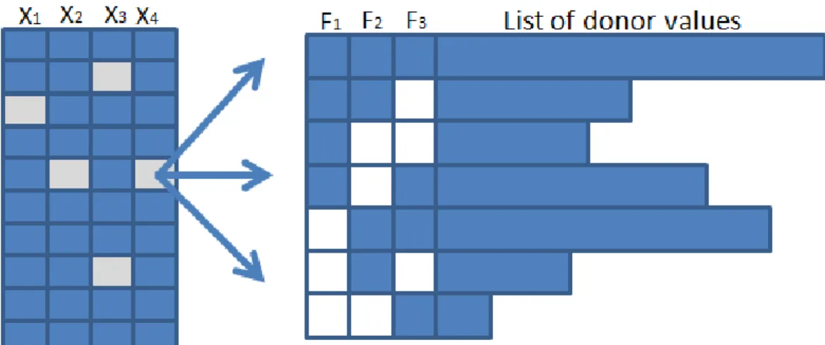
Burgette & Reiter (2010) suggest a procedure for imputing flexibly using classification and regression trees (CART) in combination with MICE. CART is a nonparametric algorithm for recursive partition respective to a dependent variable that splits the values of this variable into subgroups using the information of other variables. Those subgroups are generated with the goal to include values that are as homogenuous as possible given a defined criterion which is the least squares deviation for continuous variable and usually the Gini impurity, also re- ferred to as Gini index, for categorical variables. The homogenous value groups served as possible donor values for a missing value when CART was combined with multiple imputation as they represent the nonparametric characterization of the full conditional distribution.

The first paper about CART, used in combination with multiple imputation, was published in 2010. Since then, a large amount of articles were published about approaches using CART. Still, there is much more research to do in the field of CART or more general recursive partition algorithms. In the following, a limited literature review on current research is presented. All fields of research mentioned, that is Item-Response-Theory, handling interaction effects, clustering of individuals, e.g. in institutions, by group membership or by time, are closely related to challenges that occur when working with large-scale panel data as this is the focus of this thesis. Following this literature review, the applications that are handled in this thesis are introduced.

In the area of Item-Response-Theory approaches using trees came up in the last years. Research in the field of plausible values was made e.g. by Aßmann et al. (2014c). Mislevy (1991) presented the idea to combine multiple imputation with latent variables that were used to estimate population characteristics when individual values were missing in complex surveys. An example of a latent variable was the ”examinees’ tendencies to give correct responses to test items”, see Mislevy (1991, p.179). Aßmann et al. (2014c) used CART as a component of a Markov chain Monte Carlo procedure to impute missing values in background variables and estimated plausbile values iteratively. In the field of Rasch models, that is a model that divides personal competencies and item difficulty, Strobl et

(24)

INTRODUCTION 3

al. (2013) also used trees to impute missing data.

Doove et al. (2014) showed that CART can outclass standard applications in handling models including interaction effects when the data are multiply imputed.

The results were relativized, as the potential of CART ”depends on the relevance of a possible interaction effect, the correlation structure of the data, and the type of possible interaction effect present in the data”, see Doove et al. (2014, p.92).

Stekhoven & B¨uhlmann (2012) showed similar results of a tree-based approach handling interaction effects. Though, they used an alternative method, that is Random Forest, in using the R-package missForest instead of tree or rpart, which are packages for the usage of CART. Another difference is that Stekhoven

& B¨uhlmann (2012) focused more on mixed-type data than Doove et al. (2014).

A typical challenge of large-scale panel studies arises with the clustering of individuals within e.g. institutions, families or states. When cross-sectional data include an additional multilevel structure it has to be correctly considered when the data are imputed. This task becomes even harder when the multilevel structure is included in longitudinal data as the already existing cluster of individual measurements over time is enlarged by another level that has to be considered.

The question is whether CART can identify those different levels correctly and automatically. Some research has been done in the field of longitudinal and clustered data by Sela & Simonoff (2012) and Fu & Simonoff (2014). Sela &

Simonoff (2012) added the consideration of random effects to trees and call their approach random effects EM tree or short RE-EM tree. Though, as trees are not fitted with maximum likelihood methods, the name is misleading. The reason for the EM within that name is the alternating estimation of regression trees and random effects. See for the exact formal description of this method Sela & Si- monoff (2012, p.175). According to Sela & Simonoff (2012, p.205) the approach has the advantage that it is superior to trees ignoring the random effects within the data as it constructs different trees if the trees split on time. Additionally, it showed comparable results to linear models considering the random effects.

Fu & Simonoff (2014) adapted the algorithm of Sela & Simonoff (2012) by using a different tree approach, that is the conditional inference tree proposed by

(25)

4 INTRODUCTION

Hothorn et al. (2006) instead of CART by Breiman et al. (1984). The decision was based on the property of CART to prefer covariates with higher amounts of possible split points.

All of these approaches ignored possible missing values within the data.

In this thesis the approach of Burgette & Reiter (2010) was adapted as basis to handle nonresponse related challenges occuring within a large-scale panel study, that is the National Educational Panel Study (NEPS). Data from the NEPS were used to demonstrate two applications of CART.

First, the approach was used to analyze the unit nonresponse on metadata to decide whether nonrespondents and respondents of a study differ as correction methods should be applicated when they do. Therefore, the approach of Burgette

& Reiter (2010) was extended to a data augmentation procedure by conducting it as a component of a Markov chain Monte Carlo approach using a Gibbs Sam- pler. Here, the participation status as a dichotmous response indicator containing missing values was analyzed by a Bayesian Probit model.

Second, a large amount of variables were multiply imputed considering the high- complex filter structure of the data on the topic of household net income. There- fore, the method of Burgette & Reiter (2010) was used as a multiple imputation approach as originally inteded by them, but extended with a matrix that allows for correct implementation of all filter combinations. Thus, this matrix contained lists of proper donor values for each possible filter combination steering a variable’s values. This construct allowed for a correct implementation of the high-complex filter hierarchy within the imputation.

Then, a simulation study was conducted to show the performance of CART-based MICE on cross-sectional data. Additionally, it was checked whether a change of settings improved the performance for the given data. All analysis were based on three different data generating functions ofY.

Finally, in order to assess if CART-based MICE is suitable for imputing panel data another simulation study was conducted. The first data generating model of the previous simulation study was extended to two waves. Here, the performance on three different combinations of time-variant and time-invariant variables for

(26)

INTRODUCTION 5

a random effects model and an additional fixed effects model were tested. For both simulation studies, the quality of the multiple imputation mechanism was measured by coverages comparing the results of the before deletion, complete cases and multiply imputed data. For this purpose, coverage was defined as the proportion of 95%-confidence intervals for the estimated parameters that contained the true value.

The objective of all four applications was to assert if CART can be flexibly combined with other approaches or extended to work for various challenges of data imputation and analysis that occur within large-scale panel studies on a high-level performance.

Summarized, the focus of the first real data based applications was the imputation and analysis of unit nonresponse when auxiliary information, that could contain missings values as well, are available. The target of the second real data based application was the correct implementation of complex filter structures within the data while imputing using CART. The objective of the third application on simulated data was to evaluate the performance of the tree-based imputation on cross-sectional data and to test the influence of changed settings. The fourth application on simulated data focused on the performance of the CART-based imputation on panel data.

The thesis is organized as follows. In chapter 2, the theoretical foundations of MI, CART and the combination of CART with MICE on the one hand and data augmentation on the other hand is described. In chapter 3, an application with metadata from the NEPS on respondents and nonrespondents demonstrates the usage of CART combined with data augmentation to analyze the unit nonresponse process. Chapter 4 deals with survey data from the NEPS that is imputed using CART considering the objective to analyze household income questions considering the filter hierarchy of the data. In chapter 5, a simulation study evaluates the performance of CART-based MICE on cross-sectional data with three variables and three different types of data generating models. Another simulation study checks the performance of CART-based MICE for panel data including different time-variant and time-invariant variable combinations and a fixed effects model in chapter 6. Finally, chapter 7 concludes.

(27)

6 INTRODUCTION

(28)

Chapter 2 Theoretical foundations

In social sciences survey data typically is afflicted by missing values. Analyzing this data and ignoring the missing values can lead to invalid statistical inference.

Multiple imputation is the preferential treatment for missing values due to item nonresponse at the moment. It was invented and comprehensively shown in Rubin (1977, 1978, 1987) and many more. This chapter is at first an introduction to the multiple imputation theory. Additionally, classification and regression trees are introduced, as they ease some of the difficulties that emerge when standard multiple imputation approaches are used on complex data containing not only continuous variables, as described by Burgette & Reiter (2010). Besides the usage of CART in combination with MI, the usage in combination with data augmentation is presented as an alternative possibility to get statistically valid inference from data with missing values. Both, MI in its common application by chained equations and the iterative CART have special advantages. However, both approaches in general have limitations to address the special high-dimensional complex survey design occuring within the NEPS.

2.1 Missing Data Mechanisms and Ignorability of missing values

As a starting point, it is assumed that values are not only missing, but are missing for a reason. The reasons for the appearance of missings can be manifold. Impor-

7

(29)

8 THEORETICAL FOUNDATIONS

tant for the decision whether to impute data is the question how the mechanisms (reasons) for missing values influence the analysis of observed data.

Therefore, Rubin (1976) as well as Little & Rubin (2002, pp.14-17, 89f) defined three types of missing data mechanisms: missing completely at random (MCAR), missing at random (MAR) and not missing at random (NMAR).

For clarification of these three missing data mechanisms let Y be a n×p data matrix with i = 1, ... ,n individuals and j = 1, ... ,p variables. These variables are partially observed, that is Y_obs, and partially not observed (missing), that is Y_mis, so that Y = [Y_obs,Y_mis]. Another matrix R with elements r_ij indicates whether an element y_ij is missing (r_ij = 0) or not (r_ij = 1). The matrix R is called response indicator, see e.g.Rubin (1987, p.30). A simplified illustration to explain the usage of both matrices can be seen in figure 2.1.

Figure 2.1: Matrices Y and R indicating observed and missing values

On the left side there is the matrix as we usually see it when we look at survey data. There are cells that are observed, illustrated with darker blue. An example of a value in one of these cells is ’32’ in the first row and first column. This number includes the information that the first person (i = 1) was asked about his age (j = 1) and answered ’32 years’. The lighter blue cells indicate values that are not observed. For example a person i = 40 did not answer about the household net income j = 10. The fortieth row and tenth column would be empty or have a label for a missing value. The matrix Y is the matrix that is used as the basis for analysis of missingness. The matrixR replaces each concrete (observed) value ofY_obs with a one and each missing value, that is Y_mis, with a zero. This matrixR can be used to get an idea of the structure of the missings

(30)

THEORETICAL FOUNDATIONS 9

within the data. Additionally, combining both matrices helps to understand the definition of missing data mechanisms and how R can be explained withY. MCAR occurs when Y_obs and Y_mis can be interpreted as a random subsample of all cases. That means that the missingness does not depend on any other variables or the variable containing missing values itself. The conditional distribution f(R|Y,ψ), where ψ describes unknown parameters, can then be reduced to f(R|ψ). In a more detailed notation the equation can be written as f(R = 0|Yobs,Ymis,ψ) = f(R = 0|ψ).

MAR occurs when the Y_mis depend on observed values in the data, that is Y_obs, but not on missing values,Y_mis. The conditional distributionf(R|Y,ψ) can then be written asf(R|Y_obs,ψ). Typically, multiple imputation is conducted when the missing data mechanism is assumed to be MCAR or MAR, where the MCAR assumption is testable, see e.g. Little (1988) and the MAR assumption in general is not, see e.g. Glynn et al. (1993), Graham & Donaldson (1993) and Little &

Rubin (2002, chapter 11).

”The observed data are observed at random (OAR) if for each possible value of the missing data and the parameter ψ, the conditional probability of the observed pattern of missing data, given the missing data and the observed data, is the same for all possible values of the observed data.”, see Rubin (1976, p.582).

When the missing data are MAR and the observed data are OAR, the missing data can be described as MCAR, see Little & Rubin (2002, p.14)

NMAR occurs when the missingness can not be explained by the observed data itself. So the Y_mis depend on nonobserved values, the dropout is informative or non-ignorable, see Diggle & Kenward (1994). The conditional distribution f(R|Y,ψ) can not be simplified. Assumptions have to be made by the scientist to handle data under NMAR which can be based on ”scientific understanding or related data from other surveys”, see Rubin (1987, p.202). Furthermore, Rubin (1987, p.202) stresses that it is important to display the sensitivity under different assumptions for the response mechanism when analyzing data under the

(31)

NMAR assumption.

A very catchy description of missing data mechanisms can be found in Koller- Meinfelder (2009). Detailed information about missing data mechanisms in social science data and ways to work with them can be found in Little & Rubin (1989).

In the context of missing data mechanisms two important concepts have to be explained: distinctness and ignorability. Distinctness is formally defined as π(θ,ψ) =π(θ)π(ψ). ”From the perspective of a Bayesian statistician this means that the joint prior distribution can be split into the product of the marginal prior distributions.”, see Koller-Meinfelder (2009, p.4f). θ is the unknown (vector) parameter that steers the distribution ofY, in other words, the ’explanatory variable’ of the data analyst.

Moreover, according to Rubin (1976) and Little & Rubin (2002, p.90) the requirements for multiple imputation are that the missing data should be missing at random, the observed data should be observed at random and the parameter of the missing data process should be distinct from the parameterθwhich steers the distribution of Y. Combining those requirements the missing data mechanism should be ignorable. Thus, θ can be estimated without modelling the missing data mechanism explicitely, that is the model for R, see for example Little &

Zanganeh (2013, p.2).

The following describes typical imputation methods with focus on multiple imputation.

2.2 Imputation approaches

When missing values occur there are some ways to handle them. The most common are: Ignore them or impute them. Ignoring them by deletion of the affected cases is the default way of handling missing values in most statistical programms (van Buuren, 2012, p.8). Listwise deletion (each case with at least one missing value is deleted) and pairwise deletion (each case that is needed for the actual analysis with at least one missing value is deleted) are options when the missing data mechanism is MCAR, as it leads to unbiased estimates for the reduced data.

Compared to the original data, that include missing values, the standard errors

(32)

and significance levels for the subset of the data are often larger, see van Buuren (2012, p.8).

Imputation is a collective term that includes all techniques that replace a missing value with one or several predicted ones. About 30 years ago Sedransk (1985, p.451) ended a conference proceedings with the result that ”whenever possible, model the missing data process, do a complete data analysis and avoid imputations”. Other researchers, as for example Sande (1982), came to similar results.

Time has changed: imputation techniques were modified and became a common method. The requirements on imputation techniques are summarized by Rubin (1987), but already denoted in Rubin (1978): standard complete-data analysis methods, valid inference, display of the sensitivity of inferences. Most of the procedures allow for the mentioned standard complete-data methods, but lack for valid inferences and the display of the sensitivity of inferences.

Multiple imputation is a technique that takes the uncertainity of missing values into account and differs concerning this matter clearly from single imputation.

Nevertheless, for a better illustration and as single imputation is sufficient and reasonable in some cases, see e.g. Rao & Shao (1992), it is illustrated as well.

2.2.1 Single Imputation

There are several approaches to replace a missing value with a single value based on different assumptions about the absence of data. Deductive imputation is based on logical values, for example it is easy to understand that ’yes’ or ’no’ can be imputed to the question whether a women has children or not if she answered the question ’How many children do you have?’. Mean imputation replaces each missing value with the mean of the variable. It undererstimates the variance and biases almost every estimate besides the mean even when the missing data mechanism is MCAR. Hot-deck imputations use information of donor units, chosen for example sequentially, randomly or by nearest-neighbor approaches. For a general discussion of hot-decks, see Andridge & Little (2010). Cold-deck imputation uses information from previous time points (last observation carried forward or base- line observation carried forward), for example from a previous wave in a panel study. Another approach is regression imputation. The observed values are used

(33)

within a model and the predicted values of the fitted model serve as imputed values. The last can be unbiased even under MAR when the variables that steer the missingness are included within the regression model. For more information about those procedures see for example Lohr (2009, chapter 8.6), Little & Rubin (2002, p.61) or van Buuren (2012, p.8-13).

In general, the ’best’ single imputation method is seen in the stochastic regression imputation, which produces reasonable results, even under the MAR assumption. See for a description and a comparison to other methods Schafer

& Graham (2002, p.159-162). The approach is identical to the regression imputation, besides a residual error is added to the predicted values. For a standard linear model that error is normal distributed with mean zero and the variance estimated by residual mean square from the model, see Schafer & Graham (2002, p.159).

Single imputation techniques allow for analysis with standard complete-data techniques, but standard complete-data techniques do not differentiate between observed and imputed values. Inference can be biased and the variability that is caused by missing values is not taken into account. The latter causes bias on estimates which depend on that variability as e.g. correlations or p-values, compare e.g. Rubin (1987, p.12-15) and K.-H. Li et al. (1991). Hence, we focus on multiple imputation, as it ”retains the virtues of single imputation and corrects its major flaws”, see Rubin (1987, p.15).

2.2.2 Multiple Imputation

The idea of multiple imputation is to replace missing values by a set of plausible values drawn from the posterior predictive distribution of the missing data given the observed. Thus, a propability model is needed on the complete data: Y_mis ∼ f(Y_mis|Y_obs), compare Schafer & Olsen (1998, p.550). As it is often too complex to draw fromf(Y_mis|Y_obs) directly, a two-step procedure can be used: θ is drawn according to its observed data posterior distribution f(θ|Y_obs). Then the Y_mis are drawn according to their conditional predictive distribution f(Y_mis|Y_obs,θ), as f(Y_mis|Y_obs) =R

f(Y_mis|Y_obs,θ)f(θ|Y_obs)dθ.

It might be too complex to derive f(θ|Y_obs) as can be seen for example by

(34)

the quote from Schafer & Olsen (1998, p.549): ”Except in trivial settings, the probability distributions that one must draw from to produce proper MI’s tend to be complicated and intractable”. A solution then is to draw fromf(θ|Y_obs,Y_mis^(t)) with t as time index which leads to a data augmentation procedure, compare chapter 2.3.3.

In contrast to single imputation, multiple imputation imputesM times with m= 1, ... ,M and M ≥2. Each missing value is then replaced not by a single value, but by a vector. After those M imputations there are M complete(d) data sets on which standard complete-data methods can be applied, see e.g. Rubin (1987, p.15), Little & Rubin (2002, pp. 86-87) and Lohr (2009, chapter 8.6.7). The results of these methods can then be combined by Rubin’s combining rules which are described in chapter 2.2.4. In general, multiple imputation has important advantages compared to single imputation: 1) MI is more efficient in estimation when imputations are randomly drawn, 2) due to the variation amongst the M imputations MI takes the additional variability, caused by missing values, into account and 3) MI allows for the display of sensitivity, see Rubin (1987, p.16) and Little & Rubin (2002, pp. 85-86).

2.2.3 Imputation with chained equations

The chained equations approach, see e.g. van Buuren & Oudshoorn (1999) and van Buuren & Groothuis Oudshoorn (2011), also known as fully conditional specification (FCS), see van Buuren (2007), or sequential regressions according to Raghunathan et al. (2001), specifies an individual imputation model, that is typically a univariate general regression model, for each variable with missing values, see Azur et al. (2011). These models are iteratively chained as each dependent variable is used in the following model as one of the explanatory variables, following Little (1992) and Little & Raghunathan (1997). At first, the missing values in all variables are initialized and afterwards the algorithm iteratively runs through all specified (conditional) imputation models. The chained equations are repeated several, sayM, times. As each iteration consists of one cycle through all variables considered, the algorithm providesM completely imputed data sets, see van Buuren (2007). Before starting the multiple (sometimes called multivariate)

(35)

imputation via chained equation algorithms, the data matrix is arranged to ensure that the number of missing values per variable is ascending which is favorable in terms of convergence. The implementation of chained equation imputations are available for example inR (packagesmice andmi),SAS (packageIVEware) and Stata (packageice). Information about these implementations are available e.g.

in van Buuren & Groothuis Oudshoorn (2011), Su et al. (2011), Raghunathan et al. (2010), and Royston (2004), Royston (2005a) and Royston (2005b).

2.2.4 Rubin’s combining rules and the efficiency of an es- timate based on M imputations

When multiple imputation is conducted with for example M = 5 imputations there are five complete(d) data sets that can be analyzed. Instead of choosing one of them, the results are all used in a combined form. Rubin (1987, chapter 3) lays out the following rules for multiple imputation confidence intervals. Let θbbe the estimate of interest. Then the multiple imputation estimate ˆθ_MI can be calculated as mean of all estimates θb_m from each of the M data sets which are interpreted as completely observed for the calculation:

θˆMI = 1 M

M

P

m=1

θbm.

The total variance of the multiple imputation estimate that is needed for the width of the confindence interval as well as for tests has to be split into two com- ponents, which are the within-imputation variance and the between-imputation variance. The within-imputation varianceW is calculated analogous to the estimate above as the mean of the estimated variances for the estimate bθ :

W = 1 M

M

P

m=1var(bc θm).

(36)

The between-imputation variance B then can be described as a variance of the multiple imputation estimate θb_MI, calculated as:

B = 1 M−1

M

P

m=1

(bθ_m−θb_MI)².

The total variance T is calculated by summing both variances up, taking into account, that when the number of imputations M is increased, the simulation error for θb_MI decreases. Hence, a correction factor is added:

T =W +

1 + 1 M

B.

Using all this information a multiple imputation confidence interval can be calculated by:

θb_MI ±t_df√ T

with the degrees of freedom (df) for the quantile of the Student’s t-distribution calculated by:

df = (M−1)

1 + M·W (M + 1)B

.

For a high number of imputations (M → ∞) the normal distribution can be used instead of the Student’s t-distribution.

Typically, about M = 5 imputations are conducted before the results of the analysis of each of the imputed data sets are combined by Rubin’s rules. This number of imputations seems pretty low. But when calculating the efficiency of an estimate based on M imputations by Rubin (1987) as:

1 1 + γ

M ,

(37)

where γ is the fraction of missing information given by:

γ =

r+2 df+3

r + 1 with r = 1 +M⁻¹B

W ,

it can be seen, that for M = 5 the efficiency is higher than 90% for fractions of missing information up to 50%. A table for several M- and γ-values can be seen in Schafer & Olsen (1998). Bodner (2008) who was motivated by Royston (2004) showed an alternative table (page 666) and argued for increased numbers of imputations. His basis was a simulation study with a comparison of interpercentile ranges of 5,000 simulated 95% confidence interval half-widths, null hypothesis significance testp-values and fractions of missing information. These interpercentile ranges were interpreted as measure of variability between independent multiple imputation runs. For 95% confidence interval half-widths those interpercentile ranges for M = 5 and γ ≤ 0.50 (the exact values for γ were 0.05, 0.1, 0.2, 0.3, 0.5) lay between 0.02 and 0.30. These values are high when compared to the ranges of M = 20 which lay between 0.01 and 0.10 and very high when compared to interpercentile ranges ofM = 100 which lay between 0.0 and 0.04. Summarized, the confidence intervals are narrower and more accurate with higher numbers of imputation than with lower. This result is not suprising, but the impact of the differences in accuracy have to be considered when decid- ing about the amount of imputations in practice.

2.2.5 Using multiple imputation does not make you a wiz- ard

Using multiple imputation seems pretty charming and in a lot of cases it is.

For instance, van Buuren (2012, p.25) calls multiple imputation the ”best general method to deal with incomplete data in many fields”. But still there are some ’disadvantages’ or better said limitations and requirements that have to be considered when using it.

According to Rubin (1987, p.17f), compared to single imputation there are three (negligible) disadvantages when using multiple imputation: 1) More work and

(38)

knowledge about the procedure is needed, 2) multiply-imputed data sets need more storage space and 3) it is more difficult to analyze them (when the goal to get proper inference is ignored). The impact of these disadvantages depends on the number of imputed values. So when M is high, the impact is high. But as already mentioned in chapter 2.2.4 M = 5 is already suitable in most cases.

Otherwise as already mentioned, Bodner (2008) recommended a much higher number of imputations which depends on the fraction of missing information that has to be managed. Due to the computer power and mass storage possibilities of our time even those increased numbers can be evaluated as unproblematic.

As already mentioned in chapter 2.1, a basic requirement of multiple imputation is that the missing data mechanism is ignorable, see Rubin (1976) and Little &

Rubin (2002, p.90).

As described by Rubin (1987), Rubin (1996) and Allison (2000), the quality of the imputation depends on the ’correct’ imputation model and the congruency of the imputation model with the analyst model (’uncongeniality’), see Meng (1994).

According to e.g. Glynn et al. (1993), Graham & Donaldson (1993) and Little &

Rubin (2002, chapter 11) it can not be tested whether the missingness mechanism is NMAR or MAR.

2.3 CART used in Multiple Imputation and Data Augmentation

2.3.1 Classification and Regression Trees

Classification and regression trees (CART) were originally used in the machine learning area. Machine learning follows the idea that the computer extracts the algorithm automatically, see Alpaydin (2009, p.2). The statistical usage was adapted by Breiman et al. (1984). CART is a nonparametric algorithm for recursive partition respective to Y (dependent variable). A classification tree is used when Y is categorical (nominal or ordinal), a regression tree when Y is continuous. The basic assumption for nonparametric estimation is not a model, as in

(39)

parametric estimation, but the idea ”that similar inputs have similar outputs”, see Alpaydin (2009, p.185). CART uses nonparametric recursive binary splits to partition the data so for continuous variables the values are split in a group with values less than or equal to the splitpoint (x ≤xsplitpoint) and a group with values greater than this splitpoint (x >xsplitpoint). For categorical values two groups of values are defined, one equals a defined group of values (e.g. x = A∪B ∪C) and the other one is defined as the remaining values (e.g. x =D∪E).

In figure 2.2 there is an example of what a regression tree can look like. A classification tree would look very similar giving proportions instead of a mean value. The ovals are value groups that still have to be partitioned (pink, blue and orange). The rectangles (green and yellow) are the final groups that fulfill the stop criterion (explained later), i.e. no further partition is conducted. Those final groups are called ’final nodes’, ’end nodes’ or ’terminal nodes’ whereas the others fields (ovals) are just called ’nodes’. In the presented tree the dependent variable Y is e.g. representing the individual net income. Y is continuous and has a mean of 4,000ewith a total number of respondents ofN = 10, 000. Both, the mean and number of respondents are those of Y before any split is done, where split is a synonym for partition. The whole unpartitioned group of values is on top of the figure in pink.

A variable is chosen for the first split by CART (the rules for splitting will be explained later) which is X₁ in this example. X₁ is a categorical variable with answer choicesA,B,C,DandE. In this exampleX1 has a split point that divides all respondents of variableY that answeredA,B orC to variableX₁ in one group and all respondents that answered D or E to X₁ in another group.

The group on the left side of the tree (blue), that is the group that answeredA, B or C to variable X₁, contains 8,000 respondents and has a mean of 2,500e. The group on the right side of the tree (orange), that is the group that answered D or E to variable X₁, contains 2,000 respondents and has a mean of 10,000e. It is important to understand that the label X₁ is only about the chosen split variable and that the values ofX₁ only describe the split point. The variable that is getting more homogenous by the split is stillY and the mean and the number of respondents refer to Y as well.

(40)

VariableY mean=4,000e N=10,000 VariableX1with answersA,BandC mean=2,500e N=8,000 VariableX1with answersAandB mean=3,000e N=4,000

VariableX1with answerC mean=2,000e N=4,000

VariableX1with answersDandE mean=10,000e N=2,000 VariableX2≤45 mean=9,000e N=1,000

VariableX2>45 mean=11,000e N=1,000 Figure2.2:Exampleofaregressiontree

(41)

The group on the left side (blue) can be divided again using the same variable as another binary split of this variable X₁ is decreasing the heterogenity of the variableY for the 8,000 respondents of this group better than a split of any other variable. So the group of respondents can be divided byX1 being answered with Aor B in one group and C in the other group. The final nodes of this side are illustrated by the rectangles. Note that the number of splits on each side does not have to be the same. Finally, we have two, according to the stop criterion, most homogenous final nodes on this side with each of them containing 4,000 respondents (the number of respondents does not have to be equal, see second row: 8,000 vs. 2,000 respondents). One group has a mean of 3,000e whereas the other one has a mean of 2,000e.

On the right side of the tree (orange) we have a group of respondents that answered D or E to variable X₁. The best split to make this group become more homogenous is now a split of a continuous variable X2 at split point 45. So on the left side (yellow, on the left) we have all respondents of variable Y that answeredD or E to variableX₁ and have a maximum of 45 at variableX₂. This group contains 1,000 respondents and has a mean of 9,000e. The second group (yellow, on the right) comprises values ofX₂ that are higher than 45. This group is (randomly) as large as the other one and has a mean of 11,000e.

All four rectangle groups (green and yellow) consist of respondents that are as homogenous as they can be within their group and as heterogenous compared to the other groups based on the given split and stop criteria.

The decision whether a binary split is conducted depends on the reduction of heterogenity in the group of values by a possible split. Thus, for all possible split points the least squares deviations for continuous variables or an adequate measure for categorical variables are calculated and the split is conducted at the split point where the reduction of heterogenity is maximized. A threshold defining a minimum reduction of heterogenity serves as stop criterion. So the values within one partition get more homogenous with every split whereas the values across the partitions get more heterogenous compared to each other.

According to e.g. Breiman (1996) an adequate measure of heterogenity which

(42)

can be used as splitting criterion for categorical variables are the entropy, Gini index or the classification error:

Entropy: PG

g=1−p_glog₂p_g

Gini Index: 1−PG g=1p_g²

Classification error: 1−max{p_g}

with p_g as relative frequency of an attribute g = 1,· · · ,G within a group.

As an example for the calculation and evaluation, imagine a variable with three attributes, e.g red, blue and green. A possible split leads to the following proportions within one of the two resultings node: 0.2 (red), 0.5 (blue) and 0.3 (green). Another possible split leads to the following proportions within one of the two resulting nodes: 0.1 (red), 0.4 (blue), 0.5 (green). For simplification, only one side of the split is used as basis to calculate the heterogenity. The best split is evaluated by comparing the values of entropy, Gini index or classification error of one possible split with values of these measures of the other possible split(s). The best split is the one with the lowest resulting value, that is the lowest heterogenity.

Entropy Split 1: −0.2log₂0.2−0.3log₂0.3−0.5log₂0.5 = 1.4855

Gini Index Split 1: 1−(0.2²+ 0.3²+ 0.5²) = 0.62

Classification error Split 1: 1−0.5 = 0.5

Entropy Split 2: −0.1log₂0.1−0.4log₂0.4−0.5log₂0.5 = 1.3609

Gini Index Split 2: 1−(0.1²+ 0.4²+ 0.5²) = 0.58

Classification error Split 2: 1−0.5 = 0.5

As can be seen in this example, the entropy and the Gini index lead to a clear result, that is to prefer the second split as it leads to a lower heterogenity. The classification error does not prefer one or the other.

(43)

Alternatively to CART there are other algorithms using different numbers of splits (binary/multiway) and/or other decision rules as splitting criteria. Kim & Loh (2001) outlined some procedures when presenting their algorithm CRUISE. They mentioned CART by Breiman et al. (1984) and QUEST by Loh & Shih (1997) as binary methods. As multiway split methods FACT by Loh & Vanichsetakul (1988), C4.5 by J. R. Quinlan (1992), CHAID by Kass (1980) and FIRM by Hawkins (1997) were mentioned. Note that the algorithm C4.5 is a follower of ID3 which has not separately been mentioned by Kim & Loh (2001), see thereto J. Quinlan (1986). A newer tree-based algorithm, hence not mentioned by Kim

& Loh (2001), is CTree by Hothorn et al. (2006). The algorithm DIPOL is a follower of Cal5 by M¨uller & Wysotzki (1994).

There are many more tree-based algorithms available. Dependent on the structure of the data and the measurement criteria for the performance of those algorithms the results and the consequently preferred algorithm might differ. One of many examples of the results of a performance test can be seen from the creators of DIPOL available at the ’Technische Universit¨at Berlin’ website (https://www .ki.tu-berlin.de/menue/team/fritz_wysotzki/cal5_dipol/, date of ac- cess: 17.03.2016).

2.3.2 Nonparametric sequential classification and regres- sion trees for multiple imputation

Using MICE, conditional models have to be specified for all variables with missing data, including interactive and nonlinear relations between variables if necessary.

However, when knowledge about the conditional distribution is low or appropriate specifications involve high estimation costs, Burgette & Reiter (2010) proposed specifying the full conditional distribution within the MICE algorithm via CART (CART-based MICE). The resulting binary partition of the data along the set of conditioning variables defines the nonparametric characterization of the full conditional distribution. Hence, the final nodes can be used as donor value groups for imputation. All respondents can be assigned to one of these identified donor groups. Each missing value is imputed via a draw from the empirical distribution within this donor group using a Bayesian Bootstrap. Thus, the uncertainty of