The Performance of Panel Cointegration Methods: Results from a Large Scale Simulation Study

IHS Economics Series Working Paper 210

May 2007

The Performance of Panel Cointegration Methods: Results from a Large Scale Simulation Study

Martin Wagner

Jaroslava Hlouskova

Impressum Author(s):

Martin Wagner, Jaroslava Hlouskova Title:

The Performance of Panel Cointegration Methods: Results from a Large Scale Simulation Study

ISSN: Unspecified

2007 Institut für Höhere Studien - Institute for Advanced Studies (IHS) Josefstädter Straße 39, A-1080 Wien

E-Mail: o ce@ihs.ac.at ffi Web: ww w .ihs.ac. a t

All IHS Working Papers are available online: http://irihs. ihs. ac.at/view/ihs_series/

This paper is available for download without charge at:

https://irihs.ihs.ac.at/id/eprint/1771/

210 Reihe Ökonomie Economics Series

The Performance of Panel Cointegration Methods:

Results from a Large Scale Simulation Study

Martin Wagner, Jaroslava Hlouskova

210 Reihe Ökonomie Economics Series

The Performance of Panel Cointegration Methods:

Results from a Large Scale Simulation Study

Martin Wagner, Jaroslava Hlouskova May 2007

Institut für Höhere Studien (IHS), Wien

Institute for Advanced Studies, Vienna

Contact:

Martin Wagner

Department of Economics and Finance Institute for Advanced Studies Stumpergasse 56

1060 Vienna, Austria : +43/1/599 91-150

email: Martin.Wagner@ihs.ac.at Jaroslava Hlouskova

Department of Economics and Finance Institute for Advanced Studies Stumpergasse 56

1060 Vienna, Austria : +43/1/599 91-142 email: hlouskov@ihs.ac.at

Founded in 1963 by two prominent Austrians living in exile – the sociologist Paul F. Lazarsfeld and the economist Oskar Morgenstern – with the financial support from the Ford Foundation, the Austrian Federal Ministry of Education and the City of Vienna, the Institute for Advanced Studies (IHS) is the first institution for postgraduate education and research in economics and the social sciences in Austria.

The

aims to share “work in progress” in a timely way before formal publication. As usual, authors bear full responsibility for the content of their contributions.

Das Institut für Höhere Studien (IHS) wurde im Jahr 1963 von zwei prominenten Exilösterreichern –

dem Soziologen Paul F. Lazarsfeld und dem Ökonomen Oskar Morgenstern – mit Hilfe der Ford-

Stiftung, des Österreichischen Bundesministeriums für Unterricht und der Stadt Wien gegründet und ist

somit die erste nachuniversitäre Lehr- und Forschungsstätte für die Sozial- und Wirtschafts-

wissenschaften in Österreich. Die Reihe Ökonomie bietet Einblick in die Forschungsarbeit der

Abteilung für Ökonomie und Finanzwirtschaft und verfolgt das Ziel, abteilungsinterne

Diskussionsbeiträge einer breiteren fachinternen Öffentlichkeit zugänglich zu machen. Die inhaltliche

Verantwortung für die veröffentlichten Beiträge liegt bei den Autoren und Autorinnen.

Abstract

This paper presents results concerning the performance of both single equation and system panel cointegration tests and estimators. The study considers the tests developed in Pedroni (1999, 2004), Westerlund (2005), Larsson, Lyhagen, and Löthgren (2001) and Breitung (2005); and the estimators developed in Phillips and Moon (1999), Pedroni (2000), Kao and Chiang (2000), Mark and Sul (2003), Pedroni (2001) and Breitung (2005). We study the impact of stable autoregressive roots approaching the unit circle, of I(2) components, of short-run cross-sectional correlation and of cross-unit cointegration on the performance of the tests and estimators. The data are simulated from three-dimensional individual specific VAR systems with cointegrating ranks varying from zero to two for fourteen different panel dimensions. The usual specifications of deterministic components are considered.

Keywords

Cross-sectional dependence, estimator, panel cointegration, simulation study, test

JEL Classification

C12, C15, C23

Contents

1 Introduction 1

2 The Panel Cointegration Methods 3

2.1 Single Equation Methods ... 4

2.1.1 Tests for the null hypothesis of no cointegration ... 5

2.1.2 Estimation of the cointegrating vector ... 9

2.2 System Methods ... 12

3 The Simulation Study 16 3.1 The Performance of the Tests ... 24

3.2 The Performance of the Estimators ... 30

4 Conclusions 36

References 38

Appendix: Additional Figures and Tables 42

1 Introduction

This companion paper to Hlouskova and Wagner (2006), where panel unit root and sta- tionarity tests have been studied, investigates the properties of panel cointegration tests and estimators by means of a large scale simulation study. Our study includes both single equation and system (to be precise vector autoregression, in short VAR) tests and estimators.

The single equation tests (of the null hypothesis of no cointegration) of Pedroni (1999, 2004) and of Westerlund (2005) and the systems tests developed in Larsson, Lyhagen, and L¨ othgren (2001) and Breitung (2005) are analyzed. We do not consider single equation tests of the null hypothesis of cointegration, as such tests are bound to perform as poorly as their panel sta- tionarity counterparts. For the example of the McCoskey and Kao (1998) test, its panel stationarity test counterpart developed in Hadri (2000) has been found to exhibit devastat- ing performance in Hlouskova and Wagner (2006). Additionally performed simulations also confirm this expectation perfectly.

We have implemented several versions (i.e. with average or individual specific correction

factors, normalized, group-mean, see the description in Section 2.1.2) of both the fully mod-

ified (FM) and dynamic (D) OLS estimators, as developed in Phillips and Moon (1999) and

Pedroni (2000) for FM-OLS and in Kao and Chiang (2000), Mark and Sul (2003) and Pe-

droni (2001) for D-OLS estimation. As system estimators we include only the two-step panel

VAR estimator of the cointegrating space developed in Breitung (2005) and the one-step

or group-mean VAR estimator given by the cross-sectional average of appropriately normal-

ized individual specific Johansen estimates of the cointegrating spaces. This latter estimator

is included because it is the system counterpart to the group-mean single equation estima-

tors and is also one potential starting value for iterative system estimators. Note here that

the two-step estimator of Breitung is not an iterative estimator for the cointegrating space

because in its second step only one estimator of the cointegrating space is computed. We

abstain from including truly iterative estimators (like Larsson and Lyhagen, 1999; Groen and

Kleibergen, 2003) for the following reasons. First, we want to compare ‘similar’ estimators in

terms of (computational) complexity, i.e. we only want to compare simple regression based

estimators. Second, the proposed iterative estimators, like the Groen and Kleibergen (2003)

estimator, are (in their general version) more demanding in terms of the time dimension of

the panel due to the unrestricted set-up of the panel VAR model, see the discussion in Sec-

tion 2.2. Third, more pragmatically, iterative estimators increase the required computer time substantially, which is particularly unpleasant for large scale simulation experiments. For this latter reason we also abstain from performing even one more iterative step in Breitung’s two-step estimator.

All described tests and estimators are derived for cross-sectionally independent panels.

This for many applications unrealistic assumption is still commonly employed when devel- oping panel cointegration methods, in particular for estimation procedures. Only few and partial results concerning both cointegration testing and estimation are available for cross- sectionally dependent panels to date. Panel cointegration tests that allow for some form of cross-sectional dependence via common factors include Banerjee and Carrion-i-Silvestre (2006) and Westerlund and Edgerton (2006). The results with respect to estimation are even more scarce and include, with a different focus, (approximate) factor models as developed in Bai and Ng (2004), an extension of FM-OLS estimation to panels with short-run cross-sectional correlation developed in Bai and Kao (2005), or Kapetanios, Pesaran, and Yamagata (2006) who consider the properties of so called common correlated effects (CCE) estimators when allowing for nonstationary common factors. Additionally, several authors consider spatial or

‘economic distance’ formulations to allow for cross-sectional dependence, see e.g. Pesaran, Schuermann, and Weiner (2004).

All in all, however, the panel cointegration literature appears to be relatively nascent and partly ad-hoc with regard to cross-sectional dependence and in particular there does not seem to exist a consensus yet about successful modelling strategies for cross-sectional dependence.

Note in this respect that the present paper appears to be the first one to provide a formal definition of cross-unit cointegration, see Definition 1 in Section 3. Therefore we abstain from including methods designed for some form of cross-sectional dependence in our simulation study and focus only on some widely-used tests and estimators designed for cross-sectionally independent panels.

The data generating processes (DGPs) in the simulations are given by individual specific

three-dimensional VAR(2) processes with cointegrating ranks ranging from zero to two. Only

the cointegrating spaces are restricted to be identical for all cross-section members. We are in

particular interested in the following aspects. First, we investigate the performance of the tests

and estimators depending upon the time series and cross-section dimensions. The time series

dimension assumes the values T ∈ { 10, 25, 50, 100 } and the cross-section dimension assumes

the values N ∈ { 5, 10, 25, 50, 100 } . We only consider those combinations where T ≥ N , which results in fourteen different panel dimensions. The restriction is put in place for two reasons:

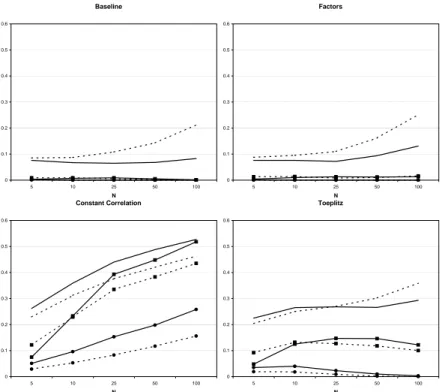
(i) For the panel VAR system methods clearly a ‘relatively’ large time series dimension is required to mitigate the substantial small sample biases of autoregressive estimation. Taking the time series dimension at least as large as the cross-sectional dimension serves as a simple heuristic lower bound. (ii) Preliminary simulations, available upon request, highlight that a cross-sectional dimension that is too large compared to the time series dimension leads to size divergence, i.e. the actual size tends to one for increasing N and fixed T smaller than N. Similar findings have been obtained for panel unit root tests in Hlouskova and Wagner (2006). Second, we investigate the impact of stable autoregressive roots approaching the unit circle on the performance of the tests and estimators. Third, we assess the effects of an I(2) component. Fourth, we study the impact of (three different forms of) short-run cross-sectional correlation on the methods’ performance. Fifth, we consider how the methods are affected by the presence of one cross-unit cointegrating relationship that is introduced in addition to the identical within-unit cointegrating relationships. Sixth, we consider the usual variety of specifications of the deterministic components.

Because we compare in part of the analysis single equation tests (where only one test is performed) with system tests (where a test sequence is performed) we use as a commonly applicable performance measure the hit rates, defined as the acceptance frequencies of the correct dimension of the cointegrating space. For the single equation tests we consider in ad- dition the power against stationary alternatives. The performance measure for the estimators is given by the gap (see (40) in Section 3.2) between the true and the estimated cointegrating spaces.

The paper is organized as follows: Section 2 describes the implemented panel cointegra- tion tests and estimators. Section 3 presents the simulation set-up, provides a discussion of different forms of cross-sectional dependence, gives a definition of cross-unit cointegration and discusses the simulation results. Section 4 draws some conclusions. An appendix containing additional figures and tables follows the main text.

2 The Panel Cointegration Methods

In this section we describe the implemented single equation and system panel cointegration

tests and estimators. We include a relatively detailed discussion for two reasons. First, the

detailed description allows the reader to see the differences and similarities across methods and tests in one place. Second, the description is intended to be detailed enough to allow the reader to implement the methods herself. In Section 2.1 the single equation methods are described and in Section 2.2 the system methods are described.

All the methods considered are so called first generation methods, as they are all formu- lated for cross-sectionally independent panels. The cross-sectional independence assumption allows for relatively straightforward asymptotic results using sequential limit theory, employed for all methods described, with first T → ∞ followed by N → ∞ . For the derivation of the test statistics the main tools applied to obtain asymptotic normality are for the pooled tests the Delta method and for the group-mean tests (where individual specific statistics are averaged) standard central limit theorems.

2.1 Single Equation Methods

The single equation methods are panel extensions of the Engle and Granger (1987) approach to cointegration analysis. The DGP is in its most general form given by

y

= α

+ δ

t + X

β

+ u

(1)

X

= X

+ ε

, (2)

observed for i = 1, . . . , N and t = 1, . . . , T . Here y

, u

∈ R , X

, ε

∈ R

, α

, δ

∈ R and β

∈ R

.

To simplify we use in slight abuse of notation the same notation for random variables (e.g. u

) and the corresponding stochastic processes (which should correctly be written as e.g. { u

}

).

Under the assumptions listed below cointegration is equivalent to stationarity of the pro- cesses u

. The single cointegrating vector is given by [1, − β

]

. When cointegration prevails we assume that the stacked processes v

= [u

, ε

]

∈ R

are cross-sectionally indepen- dent stationary ARMA processes. The ARMA assumption is stronger than required for the applicability of the functional limit theorems underlying the asymptotic analysis of the de- scribed methods. In particular the ARMA assumption guarantees the existence of finite long-run covariance matrices Ω

=

ω

Ω

Ω

Ω

. The matrices Ω

are assumed to have full

1

In the panel literature sometimes also time effects are included. We abstain from including them in both

the description and the simulation study, as they are usually extracted in the first step (similarly to the fixed

effects) and the analysis is then performed on the adjusted data. Note, however, that in general the presence

of time effects may change some of the asymptotic results.

rank, which excludes cointegration amongst the regressors X

. Note that in case of ARMA processes the long-run covariance matrices Ω

are given by a

(1)

b

(1)Σ

b

(1)

(a

(1)

)

, where a

(z)v

= b

(z)ξ

is an ARMA representation of v

with det a

(z) = 0 for | z | ≤ 1, det b

(z) = 0 for | z | ≤ 1, a

(z) and b

(z) are left co-prime and Σ

> 0 denotes the covari- ance matrix of the white noise process ξ

. For later reference we furthermore define also the conditional long-run variance ω

= ω

− Ω

Ω

Ω

and the one-sided long-run variance matrix Λ

=

j=0

E v

v

, which is partitioned according to the partitioning of Ω

.

In case of no cointegration, the processes u

are integrated of order one and the as- sumptions discussed above apply analogously to v

= [∆u

, ε

]

. Because it will be clear throughout whether the cointegration or no cointegration case is considered, using the same notation for both cases should not lead to confusion.

We consider the usual three cases for the deterministic variables: Case 1 without deter- ministic components, case 2 with only fixed effects α

and case 3 with both intercepts α

and individual specific linear time trends δ

t. The methods discussed below all allow the short-run dynamics to differ across the members of the panels. In case of cointegration, however, the usual assumption is that of a homogeneous cointegrating relation, i.e. β

= β for i = 1, . . . , N in (1). A major limitation of the single equation methods is (as in the time series case) the restriction to one cointegrating relationship.

2.1.1 Tests for the null hypothesis of no cointegration

Under the null hypothesis of no cointegration (1) is a spurious regression equation. Neverthe- less, the cross-sectional dimension allows for meaningful estimation of the so called long-run average regression coefficient for increasing cross-sectional dimension N , see Phillips and Moon (1999). Their paper establishes many of the required asymptotic results and also includes a detailed discussion concerning joint limits (with N, T → ∞ jointly) versus sequential limits (used in the other papers discussed here) with first T → ∞ followed by N → ∞ .

Pedroni. Pedroni (1999, 2004) develops in total seven different tests for the null hy- pothesis of no cointegration. Under the stated assumptions the processes u

can be written as

u

= ρ

u

+ η

, (3)

where the processes η

are stationary ARMA processes. The null hypothesis of the tests is given by H

: ρ

= 1 for i = 1, . . . , N. The pooled tests are specified against the homogeneous alternative H

: − 1 < ρ

= ρ < 1 for i = 1, . . . , N, i.e. these tests are shown to be consistent against the homogeneous alternative which restricts the first-order serial correlation coefficient ρ of the processes u

to be identical for i = 1, . . . , N . The group-mean tests, based on cross-section averages of individual estimators of ρ

, are specified (i.e. consistent) against the heterogeneous alternative H

: − 1 < ρ

< 1 for i = 1, . . . , N

and ρ

= 1 for i = N

+1, . . . , N.

For consistency of the group-mean tests, a non-vanishing fraction of the individual units has to be stationary under the alternative, i.e. lim

N

/N > 0.

Of course, the tests are computed with estimated ˆ u

in place of the unobserved errors u

. In particular OLS residuals of (1) can be chosen, see Phillips and Ouliaris (1990) in the time series case, and a similar endogeneity correction factor (ω

) appears, see Phillips and Moon (1999) for a discussion of the properties of the OLS estimator of β

. The estimator

ˆ

ω

is given by the estimator of the long-run variance of the residuals, ˆ η

say, of an OLS regression of ∆y

on the differenced deterministic components and ∆X

. The estimate ˆ ω

can be obtained by using a kernel estimator, see Andrews (1991) or Newey and West (1987) or alternatively by fitting an ARMA or AR model to ˆ η

(and computing the long-run variance model based).

The correction for serial correlation can be handled either non-parametrically (following Phillips and Perron, 1988) or by using ADF type regressions. Let us start with the non- parametric tests. Denote the residuals of the OLS regressions ˆ u

= ρ

u ˆ

+ µ

by ˆ µ

. Further, denote their estimated variances by ˆ σ

and their estimated long-run variances by

ˆ

ω

. Then, the serial correlation factors are given by ˆ λ

=

(ˆ ω

− σ ˆ

). For later use we also define ˆ ω

=

i=1

ω ˆ

/ˆ ω

.

With the defined quantities the following pooled test statistics can be computed: the variance ratio statistic P P

, the test based on the autoregressive coefficient P P

, and the test based on the t-value of the autoregressive coefficient P P

.

We write the test statistic below including scaling factors that display the convergence properties of the different components of the test statistics. This allows for a simple understanding of the construction principles, whereas in an actual computation of the test statistics these scaling factors (partly) drop out.

2P P

is used here as acronym for Pedroni pooled test. Below we use

as acronym for Pedroni group-mean

test.

The essential parts (i.e. without centering and scaling factors, see below) of the pooled test statistics are given by

P P

= N

N

i=1

ˆ ω

T

ˆ u

(4)

P P

= N

N

i=1

ω ˆ

T

t=2

u ˆ

∆ˆ u

− λ ˆ

N

i=1

ω ˆ

T

t=2

u ˆ

(5)

P P

= N

N

i=1

ω ˆ

T

t=2

u ˆ

∆ˆ u

− λ ˆ

ˆ

ω

N

i=1

ω ˆ

T

t=2

u ˆ

. (6)

The ADF-type test P P

is based on autoregressions to correct for serial correlation. Em- ploying the Frisch-Waugh theorem, two auxiliary regressions are performed

∆ˆ u

=

Ki

k=1

γ

∆ˆ u

+ ζ

(7)

ˆ

u

=

Ki

k=1

γ

∆ˆ u

+ ζ

, (8) where the lag lengths K

are determined in our simulations using AIC in ∆ˆ u

= ρ

u ˆ

+

k=1

γ ˜

∆ˆ u

+ ˜ ζ

. Denote the OLS residuals of the above equations (7) and (8) by ˆ ζ

and ζ ˆ

, the residuals from the regressions ˆ ζ

= ρ

ζ ˆ

+ θ

by ˆ θ

and their estimated variances (needed later) by ˆ σ

. Furthermore define ˆ σ

=

i=1

t=Ki+2

θ ˆ

. The essential part of the ADF-type statistic is then given by

P P

= N

N

i=1

ω ˆ

T

t=Ki+2

ζ ˆ

ζ ˆ

ˆ

σ

N

i=1

ω ˆ

T

t=Ki+2

ζ ˆ

. (9)

By construction, for N = 1 these statistics coincide with their time series counterparts.

Asymptotic normality using sequential limit theory can easily be established for the above test statistics by applying the so called Delta method (this requires knowledge of the (asymptotic) means and variances of the building blocks, which are obtained for practical purposes by simulation). The mean and variance correction factors, M

(r, s, l) and V

(r, s, l) depend upon the test considered (r ∈ { σ, ρ, t, df } ), the case concerning the deterministic variables (s ∈ { 1, 2, 3 } ) and upon the number of regressors l, i.e.:

P P

= P P

− N

M

(r, s, l)

(V

(r, s, l))

⇒ N (0, 1).

Pedroni develops three group-mean tests against the heterogeneous alternative. These are:

a test based on the first order serial correlation coefficient P G

, a test based on its t-value P G

and again an ADF-type test P G

. The essential parts of the test statistics are given by

P G

= N

i=1

P G

= N

i=1T⁻¹_T

t=2

(

)

T⁻²_T

t=2ˆu²_it−1

P G

= N

i=1

P G

= N

i=1T⁻¹_T

t=2

(

)

ˆ

ω_µi

(

t=2uˆ²_it−1

)

P G

= N

i=1

P G

= N

i=1

T⁻¹_T

t=Ki+2ζˆ1itζˆ2it

ˆ σ_θi

T⁻²_T

t=Ki+2ζˆ_2it² _1/2

.

(10)

Appropriately centered and scaled group-mean test statistics converge to the standard normal distribution in the sequential limit by applying the central limit theorem to the i.i.d. (across N) sequences, i.e.:

P G

=

(VP G(r,s,l))^1/2

= N

i=1P G^o_r,i−MP G(r,s,l)

(VP G(r,s,l))^1/2

⇒ N (0, 1), (11) with r ∈ { ρ, t, df } , s ∈ { 1, 2, 3 } and l the number of regressors. The correction factors for all discussed tests are tabulated in Pedroni (1999) for two to seven regressors.

Kao (1999) develops similar tests to those of Pedroni for the special case of panels where not only the vectors β

are assumed to be identical, but also the dynamics of the error pro- cesses v

are assumed to be identical for i = 1, . . . , N.

Westerlund. Westerlund (2005) develops two simple non-parametric tests that extend the Breitung (2002) approach from the time series to the panel case. One test, W P , is pooled and hence specified against the homogeneous alternative and the other one, W G, is a group- mean test against the heterogeneous alternative. As for the Pedroni tests, the OLS residuals

ˆ

u

from (1) are the starting point. Denote with ˆ r

=

t=1

u ˆ

, with ¯ r = N

i=1

ˆ r

and with ˆ e

=

j=1

u ˆ

. The essential parts of the test statistics are then given by W P

= N

N

T

¯ r

T

ˆ e

(12)

W G

= N

T

ˆ r

T

ˆ e

. (13)

Applying the Delta method to W P

and a central limit theorem to W G

(easily seen again by writing W G

= N

i=1

W G

) leads to asymptotic standard normality under the null

hypothesis in the sequential limit when applying appropriate mean and variance correction factors, i.e.:

W P = W P

− N

M

(r, s, l)

(V

(r, s, l))

⇒ N (0, 1) W G = W G

− N

M

(r, s, l)

(V

(r, s, l))

⇒ N (0, 1).

2.1.2 Estimation of the cointegrating vector

In this subsection we assume that the processes u

are stationary and hence that cointegra- tion prevails for all cross-section members. As mentioned at the beginning of the section, a difference to the time series case is that the cross-section dimension implies that the (pooled) OLS estimator of β in (1) (also when the β

are not restricted to be identical for i = 1, . . . , N ) converges to a well-defined limit also in the spurious regression and the (heterogeneous) coin- tegration cases. This limit is given by the so called average long-run regression coefficient (for a detailed discussion and the precise assumptions see Theorems 4 and 5 of Phillips and Moon, 1999). As in the time series case, the limiting distribution of the OLS estimator depends upon nuisance parameters. For the rest of this section we focus on the case of homogeneous cointegration, i.e. β

= β for i = 1, . . . , N , to be estimated by panel methods. Consequently, later on we also consider the system methods for the estimation of a cross-sectionally identical cointegrating space.

As in the time series case regressor endogeneity and serial correlation of the errors, which lead to nuisance parameter dependency of the limiting distribution of the OLS estimator, can be handled in two ways, by either performing fully modified OLS estimation (cf. Phillips and Hansen, 1990) or by performing dynamic OLS estimation (cf. Saikkonen, 1991). As for the tests both a pooled and a group-mean approach are possible. Furthermore, also the correction factors can be individual specific or cross-sectionally averaged.

In the description of the estimation procedures we focus on the case with fixed effects only (i.e. case 2).

Denote with ¯ y

=

t=1

y

and with ¯ X

=

t=1

X

and denote the demeaned variables by ˜ y

= y

− y ¯

and ˜ X

= X

− X ¯

.

3

The other two cases are entirely similar. In case 1 the original variables are taken as inputs, and in case 3

the variables are demeaned and detrended at the outset of the procedure. The limiting distributions change

accordingly, between case 1 on the one hand and cases 2 and 3 on the other. Also, intercepts in the regressors,

i.e.

=

+

+

can be accommodated.

FM-OLS. Obtain estimators ˆ Ω

, ˆ Ω

, ˆ Λ

and ˆ Λ

from the residuals [ˆ u

, ε

]

.

Defining the endogeneity corrected variable ˜ y

= ˜ y

− Ω ˆ

Ω ˆ

∆ ˜ X

leads to the pooled FM-OLS estimator:

β ˆ

=

i=1

X ˜

X ˜

i=1

X ˜

y ˜

− N T ( ˆ Λ

)

, (14)

with ˆ Λ

= ˆ Λ

− Ω ˆ

Ω ˆ

Λ ˆ

.

Phillips and Moon (1999) use in their formulation of the FM-OLS estimator averaged correction factors, e.g. ˆ Ω

=

i=1

Ω ˆ

and similarly constructed ˆ Ω

, ˆ Λ

, ˆ Λ

and ˆ Λ

.

The limiting distribution of the FM-OLS estimator (see e.g. Theorem 9 of Phillips and Moon, 1999) is given by:

N

T( ˆ β

− β) ⇒ N (0, 6ω

Ω

) (15) with ω

= lim

i=1

ω

and Ω

= lim

i=1

Ω

. For case 1 without deter- ministic components the factor 6 in the limiting distribution has to be replaced by the factor 2. Note that the limiting covariance matrix is composed of cross-sectional averages.

Standard (up to the factor 2 or 6, depending upon case considered) normally distributed pooled FM-OLS estimators are also easily constructed. These are popular due to their im- plementation in freely available software. Define ˜ y

= ˆ ω

y ˜

− (ˆ ω

I

− Ω ˆ

)X

β, ˆ X ˜

= ˆ Ω

X ˜

and ˆ Λ

= ˆ ω

Λ ˆ

Ω ˆ

, where ˆ β denotes the LSDV estimate of β. Then, the normalized FM-OLS estimator is given by

β ˆ

=

i=1

X ˜

X ˜

i=1

X ˜

y ˜

− N T ( ˆ Λ

)

(16) and it holds that N

T ( ˆ β

− β ) ⇒ N (0, 6I

), where the factor 6 has to be replaced by the factor 2 in case no deterministic components are included in (1).

Group-mean FM-OLS estimation is considered in Pedroni (2000). The group-mean FM- OLS estimator is (in its unnormalized form) given by the cross-sectional average of the indi- vidual FM-OLS estimators of β:

β ˆ

= 1 N

⎛

⎝

t=1

X ˜

X ˜

t=1

X ˜

y ˜

− T ( ˆ Λ

)

⎞

⎠ . (17)

4

By assumption

= ∆

. Note also that because we assume a homogeneous cointegrating relationship instead of the OLS residuals also the residuals from an LSDV regression (which puts the restriction

=

in place) can be used.

5

Similar results are also contained in Pedroni (2000) and Kao and Chiang (2000).

D-OLS. We now turn to dynamic OLS estimation of the cointegrating relationship, as discussed in Kao and Chiang (2000) and Mark and Sul (2003). The idea of D-OLS estimation is to correct for the correlation between u

and ε

by including leads and lags of ∆X

as additional regressors in the cointegrating regression. As in the time series case the number of leads and lags (in general) has to increase with the time dimension of the panel at a suitable rate to induce asymptotic uncorrelatedness between the noise processes in the lead and lag augmented cointegrating regression and ε

. Thus, considering again case 2, let the augmented cointegrating regression be given by

˜

y

= X ˜

β +

pi

j=−pi

∆ ˜ X

γ

+ u

(18)

= X ˜

β + ˜ Z

γ

+ u

,

where the last equation defines ˜ Z

and γ

. The pooled D-OLS estimator for β is then obtained from OLS estimation of the above equations (18). Let ˜ Q

= [ ˜ X

, 0

, . . . , 0

, Z ˜

, 0

, . . . , 0

]

∈ R

, where the variables ˜ Z

are at the i-the position in the second block of the regressors. Using this notation we obtain

⎡

⎢ ⎢

⎢ ⎣ β ˆ

ˆ γ

.. . ˆ γ

⎤

⎥ ⎥

⎥ ⎦ =

i=1

Q ˜

Q ˜

i=1

Q ˜

y ˜

. (19)

Mark and Sul (2003) derive the asymptotic distribution of ˆ β

that has a ‘sandwich’ type limit covariance matrix. Denote with ¯ V = lim

i=1

ω

Ω

. Then it holds that

N

T ( ˆ β

− β) ⇒ N (0, 6Ω

V ¯ Ω

). (20) Kao and Chiang (2000) discuss a normalized version of the D-OLS estimator that cor- responds to ˆ β

. This estimator, ˆ β

say, is obtained when in the above discussion of the D-OLS estimator ˜ y

and ˜ X

are replaced by ˜ y

and ˜ X

. These changes lead to an estimator with a limiting covariance matrix proportional to the identity matrix.

Pedroni (2001) considers a group-mean D-OLS estimator. Denote with ˜ R

= [X

, Z ˜

]

and estimate (separately for i = 1, . . . , N)

β ˆ

ˆ γ

=

t=1

R ˜

R ˜

t=1

R ˜

y ˜

. (21)

Then the group-mean D-OLS estimator is given by ˆ β

=

i=1

β ˆ

. Also this estimator can be computed in a normalized version. The limiting distributions coincide with the limiting distributions of the corresponding pooled estimators.

2.2 System Methods

The second strand of the panel cointegration literature is based on panel extensions of VAR cointegration analysis (see Johansen, 1995). Compared to the single-equation methods sev- eral differences are worth mentioning. First, the systems approach allows to model multiple cointegrating relationships. Second, the cointegrated VAR approach allows to incorporate a richer specification concerning (restricted) deterministic components considered relevant in the applied cointegration literature. Third, specifying a parametric model allows to also consider the dynamic (short-run) characteristics of the data, which are treated as nuisance parameters in the non-parametric single equation approaches. Being based on VAR estimates, the system methods are, as their time series building block, subject to substantial biases for short time series. Thus, for practical applications the time series dimension has to be suffi- ciently large. This is also required for the reason that specifying a dynamic model requires the estimation of more parameters and hence in general more data. In this respect one, however, has to take into account that also an accurate estimation of the long-run variances used in the nonparametric methods discussed above also requires a sufficiently large time dimension.

Without imposing any homogeneity assumption the panel VAR DGP is given in error correction form by

∆Y

= C

+ C

t + α

β

Y

+

pi

j=1

Γ

∆Y

+ w

, (22) with Y

∈ R

, C

, C

∈ R

, α

, β

∈ R

with full rank, Γ

∈ R

and w

cross- sectionally independent m-dimensional white noise processes with covariance matrices Σ

> 0.

To ensure that the processes described by (22) are (up to the deterministic components) I(1) processes, the matrices α

Γ

β

have to be invertible, where α

∈ R

, β

∈ R

are full rank matrices such that α

α

= 0 and β

β

= 0 and Γ

= I

−

j=1

Γ

.

In this case the space spanned by the columns of the matrix β

, i.e. sp { β

} , is the k

- dimensional cointegrating space of unit i.

6

One possible choice is given by

=

(α

)

and similarly for

.

7

The integer

is often referred to as cointegrating rank. Please note that

as used in this sub-section

In the VAR cointegration literature the following five specifications concerning the deter- ministic components are usually discussed. Case 1 is without any deterministic components.

In case 2 restricted intercepts of the form C

= α

τ

are contained (in the cointegrating space) and case 3 includes unrestricted intercepts C

that induce linear time trends in Y

. In case 4 unrestricted intercepts and restricted trend coefficients C

= α

κ

are included, this allows for linear trends in both the data and the cointegrating relationships. Finally in case 5 unrestricted intercepts and trend coefficients are included. The latter case leads to quadratic time trends in the data and appears to be not too relevant for economic time series. For this reason we do not consider this case in our simulations. A detailed discussion of the specifications of the deterministic variables is given in Johansen (1995, Section 5.7).

The statistical analysis, i.e. parameter estimation (via reduced rank regression) as well as testing for the cointegrating rank, is well-developed and known for all the listed cases (see Johansen, 1995) and therefore we do not repeat a discussion of this well-known procedure here.

Larsson, Lyhagen, and L¨ othgren. Larsson, Lyhagen, and L¨ othgren (2001) consider testing for cointegration in the above framework under the assumption that Π

= α

β

= αβ

= Π for i = 1, . . . , N .

The null hypothesis of their test is H

: rk(Π

) = k for i = 1, . . . , N. The test is consistent against the alternative hypothesis that H

: rk(Π

) = m for a non-vanishing fraction of cross-section members. The construction of this test statistic is similar to Im, Pesaran, and Shin (2003) and hence the test statistic is given by a suitably centered and scaled version of the cross-sectional average of the individual trace statistics. Thus, denote with LR

(k | m) the trace statistic for the null hypothesis of a k-dimensional cointegrating space for unit i, where the superscript s indicates the specification of the deterministic components.

Using a central limit theorem in the cross-sectional dimension and the appropriate mean and variance correction factors implies that under the null hypothesis

LLL

(k | m) = N

LR

(k | m) − E (LR

(k | m))

V ar(LR

(k | m)) ⇒ N (0, 1) (23)

does not coincide with

used in the description of the single equation methods, where the single cointegrating vector is given by [1

]

. Also for notational brevity we will not always differentiate between the matrix

and the space spanned by its columns. We are confident that this does not lead to any confusion.

8

As we shall see below, their test is simply based on the cross-sectional average of the Johansen trace

statistic, where this restriction is not imposed anywhere in the construction of the test statistic. However, they

have only established the asymptotic distribution of their test statistic under this assumption (see Assumption

3’ and Theorem 1 of Larsson, Lyhagen, and L¨ othgren, 2001).

in the sequential limit T → ∞ followed by N → ∞ .

For T → ∞ the expressions E (LR

(k | m)) and V ar(LR

(k | m)) converge to the limit of the expected value respectively variance of the trace statistic (corresponding to the case s considered). In principle also finite T correction factors (for different lag lengths and numbers of variables), see again Im, Pesaran, and Shin (2003), can be obtained by simulation. Our simulation study is based on the asymptotic correction factors. Note already here that the simulation results indicate that using finite T correction factors may be beneficial.

Breitung. Breitung (2005) proposes a 2-step estimation (and related test) procedure that extends the Ahn and Reinsel (1990) and Engle and Yoo (1991) approach from the time series to the panel case. Breitung considers the homogeneous cointegration case where only the cointegrating spaces are assumed to be identical for all cross-section members. In the first step of his procedure the parameters are estimated individual specifically and in the second step the common cointegrating space β is estimated in a pooled fashion.

For simplicity we describe the method here for the VAR(1) model without deterministic components. In the general case lagged differences as well as (restricted) deterministic com- ponents are treated in the usual way and are concentrated out in the first step, as described in Johansen (1995). Thus, consider

∆Y

= α

β

Y

+ w

(24)

Pre-multiplying equations (24) by T

= (α

Σ

α

)

α

Σ

leads to

(α

Σ

α

)

α

Σ

∆Y

= β

Y

+ (α

Σ

α

)

α

Σ

w

(25) T

∆Y

= β

Y

+ T

w

(26)

∆Y

= β

Y

+ w

, (27)

where the last equation defines the variables with superscript

. Note also that E w

(w

)

= (α

Σ

α

)

. Now use the normalization β = [I

, β

]

and partition Y

= [(Y

)

, (Y

)

]

with Y

∈ R

and Y

∈ R

. Using this notation we can rewrite the above equation as

∆Y

− Y

= β

Y

+ w

. (28)

9

The authors actually derive this result for a so called

limit with

0, i.e. for sequences of (

) where

grows suitably slower than

.

10

Note that in the first step individual specific estimators of all parameters are obtained and used, including

first step estimators of ˆ

.

Breitung suggests to estimate (28) by pooled OLS using the estimate ˆ T

= ( ˆ α

Σ ˆ

α ˆ

)

α ˆ

Σ ˆ

based on the Johansen estimators. Note that, given that the covariance structure of the errors in (28) is known (and an estimate is available), also pooled feasible GLS estimation of (28) is an option.

Breitung’s estimation procedure stops here. However, an iterative estimator is easily conceived, based on the above procedure. With the estimated ˆ β

, one can re-estimate the individual specific parameters in (24) by running separate OLS regressions. With the new estimates of α

and Σ

(in the VAR(1) example without deterministics) then again equa- tion (28) can be estimated. This process can be continued until convergence occurs. Such an iterative procedure corresponds to the iterative estimator proposed in Larsson and Lyhagen (1999).

The only difference is that in the first step Larsson and Lyhagen (1999) propose to take as an initial estimator ˆ β =

ˆ

i=1

β ˆ

, where ˆ β

denotes the Johansen estimator of the cointegrating space for cross-section unit i.

We refer to this initial estimator later on as one-step or group-mean VAR estimator, in analogy to the group-mean FM-OLS and D-OLS estimators discussed above.

Breitung shows that the two-step estimator, ˜ β

say, is asymptotically normally distributed N

T vec( ˜ β

− β

) ⇒ N (0, Ω

⊗ Σ

), (29) with ⊗ denoting the Kronecker product, Ω

= lim

lim

E

i=1

t=1

Y

(Y

)

and Σ

= lim

i=1

(α

Σ

α

)

.

The test Breitung proposes for the null hypothesis of rk(β) = k is based on Saikkonen (1999). The difference to the Larsson, Lyhagen, and L¨ othgren (2001) test is that Breitung’s test incorporates the homogeneity restriction β

= β for i = 1, . . . , N in the construction of the

11

Note, however, that Larsson and Lyhagen (1999) consider a much more general specification (using again the VAR(1) example) of the form

⎡

⎢⎣

∆

.. .

∆

⎤

⎥⎦

=

⎡

⎢⎣

α11 . . . α1N

.. . . . . .. .

⎤

⎥⎦

⎡

⎢⎣

β

0

0

.. . 0

⎤

⎥⎦

⎡

⎢⎣ Y1t−1

.. .

⎤

⎥⎦

+

⎡

⎢⎣ w1t

.. .

⎤

⎥⎦

, with a full covariance matrix of the stacked noise process. It is not clear whether such an – up to

the cointegrating space – unrestricted VAR process for the stacked data should really be interpreted as a panel model, as the loose parameterization implies that the time dimension of the panel has to be large compared to the cross-sectional dimension. Also Groen and Kleibergen (2003) consider a relatively general panel VAR model that seems to require panel data sets with a large time dimension, as in their simulations they consider a bivariate example for

= 1

3

5 and

= 1000.

12

Before averaging the estimators over the cross-section dimension it is important to impose a common

normalization, e.g. ˆ

= [

ˆ

]

.