Gioele Zardini Control Systems II FS 2018
Lecture 1: Feedback Control Loop
Remark. This exercise contains much algebraic calculus and has not standard difficulty.
If you want to challenge yourself with a model of a real system, you should try to solve that. This is not the complication level one would require in an exam!
Example 1. Your are given an inverted pendulum, depicted in Figure 1. The pendulum
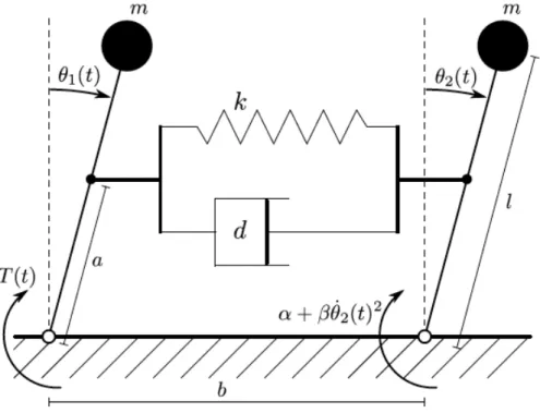
Figure 1: Inverted Pendulum.
consists of two point masses mon two rods of length l. The rods are supported in a pivot on a horizontal plane. At distanceafrom the pivot, they are connected by a spring-damper system. The spring has spring constant k. Its neutral position is at θ1 =θ2 = 0. In the pivot of the left mass, an external torque T(t) can be applied. In the right pivot, there is a disturbance torque of the form α+βθ˙2(t)2. The differential equations representing the dynamics of the described system are:
ml2θ¨1(t) = mglsin(θ1(t)) +acos(θ1(t))F(t) +T(t)
ml2θ¨2(t) = mglsin(θ2(t))−acos(θ2(t))F(t) +α+βθ˙2(t)2, (0.1) where F(t) is the force resulting from the spring-damper system.
a) Calculate the force F(t).
b) Compute the equilibrium point of the system. Let ¯θ2 = 0.
c) Which vector could be a correct state space vector?
1
Gioele Zardini Control Systems II FS 2018
d) Let now α = 0. Linearize the system around the equilibrium point ¯θ1 = ¯θ = ¯T = 0 and derive the continuous-time state-space description
˙
x(t) = Ax(t) +Bu(t)
y(t) = Cx(t) +Du(t), (0.2)
whereu(t) =T(t)−T¯, and y(t) =θ1(t)−θ¯1. Hint: Consider small angle variations.
Solution.
a) Using concepts on mechanics, one can compute F(t) =ka[sin(θ2(t))−sin(θ1(t))] +dah
cos(θ2(t)) ˙θ2(t)−cos(θ1(t)) ˙θ1(t)i
, (0.3) The new equations of motion read
θ¨1 = mglsin(θ1) +acos(θ1)F(t) +T ml2
= g
l sin(θ1) + a2
ml2 cos(θ1)h
k(sin(θ2)−sin(θ1)) +d
cos(θ2) ˙θ2−cos(θ1) ˙θ1i + T
ml2 θ¨2 = mglsin(θ1)−acos(θ2)F(t) +α+βθ˙22
ml2
= g
l sin(θ1)− a2
ml2 cos(θ2)h
k(sin(θ2)−sin(θ1)) +d
cos(θ2) ˙θ2−cos(θ1) ˙θ1i
+ α+βθ˙22 ml2 , (0.4) where I dropped the time dependencies for simplicity.
b) At equilibrium holds ˙θ1(t) = ˙θ2(t) = ¨θ1(t) = ¨θ2(t) = 0. By plugging these informations into the equations of motion one gets
mglsin(θ1(t))−a2kcos(θ1(t)) sin(θ1(t)) +T(t) = 0
a2ksin(θ1(t)) +α= 0. (0.5) From this, it follows
θ¯1 = arcsin
− α a2k
T¯=mgl α
a2k −αcos
arcsin
− α a2k
.
(0.6)
Remark. Here, we are considering ¯T as the equilibrium value of an input (i.e. ¯u).
c) Because of the second derivatives, a state augmentation is needed. A good choice for the state space vector is
x= θ1(t) θ2(t) θ˙1(t) θ˙2(t)|
. (0.7)
d) With the new α we have ¯θ2 = 0, ¯θ1 = 0, ¯T = 0. The new system reads
x(t) =
x1(t) x2(t) x3(t) x4(t)
=
θ1(t)−θ¯1
˙ x1(t) θ2(t)−θ¯2
˙ x3(t)
=
θ1(t)
˙ x1(t) θ2(t)
˙ x3(t)
, u(t) =T(t)−T¯=T(t). (0.8)
2
Gioele Zardini Control Systems II FS 2018
By writing ˙x(t) = f(x(t), u(t)), one identifies (always dropping the time dependencies and writing cos asc and sin as s)
f(x(t), u(t)) =
x2
g
ls(x1) + mla22c(x1) [k(s(x3)−s(x1)) +d(c(x3)x4−c(x1)x2)] + mlu2
x4
g
ls(x1)− mla22c(x3) [k(s(x3)−s(x1)) +d(c(x3)x4−c(x1)x2)] + α+βxml224
. (0.9) Hence, one can now derive the state matrices with the formalism
A = ∂f(x(t), u(t))
∂x(t)
x(t)=¯x,u(t)=¯u, B = ∂f(x(t), u(t))
∂u(t)
x(t)=¯x,u(t)=¯u
.
(0.10)
The matrices hence read
A=
0 1 0 0
g
l − aml2k2 −mla2d2
a2k ml2
a2d ml2
0 0 0 1
a2k ml2
a2d ml2
g
l −mla2k2 −mla2d2
,
B =
0
1 ml2
0 0
,
C= 1 0 0 0 , D= 0,
(0.11)
where small angles approximations have been used.
3