Total frame potential and its applications in data clustering

Total Frame Potential and its Applications in Data Clustering

Dissertation

zur Erlangung des akademischen Grades eines Doktors der Naturwissenschaften

Der Fakult¨ at f¨ ur Mathematik der Technischen Universit¨ at Dortmund

vorgelegt von

Tobias Springer

im Jahr 2013

Erstgutachter: Prof. Dr. Joachim St¨ockler Zweitgutachterin: Prof. Dr. Katja Ickstadt Dritter Pr¨ ufer: Prof. Dr. Christoph Buchheim Wissenschaftlicher Mitarbeiter: Dr. Thorsten Camps

Datum des Pr¨ ufungskolloquiums: 26.11.2013

Abstract

For the statistical analysis of microarray gene expression data, the clustering of short time series is an important objective in order to identify subsets of genes sharing a temporal ex- pression pattern. An established method, the Short Time Series Expression Miner (STEM) by Ernst et al. ([Erns 05]), assigns time series data to the closest of suitably selected proto- types followed by the selection of significant clusters and eventual grouping. This algorithm identifies each time series by a corresponding vector in R

which contains the data expressions at d ∈ N not necessarily equidistantly distributed points in time. In order to qualify for the term “short” time series, the number d is supposed to be small, e.g. d ≤ 12.

For the clustering of normalized d-dimensional data Y = { y

}

we propose to minimize the Penalized Frame Potential

F

(Θ, Y ) = TFP(Θ) − α

m

X

ℓ=1

j=1,...,N

max h y

, θ

i (1) on the m-fold unit sphere for the regularization parameter α ≥ 0. The functional contains the “Total Frame Potential” (TFP) whose minimizers are exactly the Finite Unit Norm Tight Frames (FUNTFs), see Benedetto and Fickus ([Bene 03]), and includes a data-driven com- ponent for the selection of prototypes. We show that the solution of the corresponding con- strained optimization problem is naturally connected to the spherical Dirichlet cells

D

= (

v ∈ R

: k v k

= 1, y

= arg max

1≤k≤N

h y

, v i )

of the given normalized data. Furthermore, the minimizers of F

are, given that α > 0, in the interior of the Dirichlet cells and the objective function F

is differentiable in the minimum with the extremal condition

4T T

T + 2T Λ = αY

where T , Y

∈ R

have normalized columns and Λ = diag(λ

, . . . , λ

) contains the Lagrange multipliers from a corresponding constrained minimization problem.

The general problem is closely related to the search for point configurations on the unit sphere

like in Tammes’ ([Tamm 30]) or Thomson’s Problem ([Thom 04]). Moreover, the minimization

problems in matrix completion (see e.g. Cand`es and Tao in [Cand 10] or Mazumder, Hastie and Tibshirani in [Mazu 10]).

The idea of using the frame potential in combination with a data-dependent term for opti- mization was originally proposed by Benedetto, Czaja and Ehler ([Bene 10]) for finding sparse coefficient representations. First results of our proposed method were published by Springer, Ickstadt and St¨ockler ([Spri 11]).

The thesis presents the motivation of our approach by introducing the STEM algorithm for

data clustering and outlining the connection to a proposal in [Bene 10]. We give an overview

over the development in the theory of Finite Unit Norm Tight Frames. Moreover, we analyze

the features of the Penalized Frame Potential and illustrate relations to other well-known

optimization problems in the theory of Compressive Sensing. Finally, we present numerical

results on the implementation of the functional by application on real and simulated data.

Acknowledgements

First and foremost, I would like to give a few words to the people who have contributed to this thesis in different ways. I am indebted to Prof. Dr. Joachim St¨ockler who was an encouraging and motivating advisor. The numerous meetings were a great source of inspiration and almost always led to new insights. I am also grateful to Prof. Dr. Katja Ickstadt for supporting the ideas of implementing new methods and for agreeing to be a reviewer for this thesis.

Another important factor was the team at the Lehrstuhl f¨ ur Approximationstheorie – especially PD Dr. Maria Charina, Tobias Kloos and Dr. Katrin Siemko – who created a very pleasant working atmosphere during the last four years. Included is our secretary Christine Mecke for the morning coffee and the help on administrative issues.

Since my family has always been helpful during the last years, I also thank my parents Susanne

and Detlef Springer who always encouraged me in various ways and Alina St¨oteknuel for being

constantly supportive in all aspects. Finally, the help of my good friends Hendrik Blom and

Arne Hauner in preparation for my thesis defense should not go unmentioned.

Contents

1 Introduction 1

2 Frames 5

2.1 Finite Frames . . . . 8 2.2 Critical Points of the Frame Potential . . . . 13 2.3 Spectrum and Non-Tightness . . . . 21

3 Cluster Algorithms for Short Time Series 23

3.1 On the Short Time Series Expression Miner . . . . 25 3.2 A Note on Tammes’ Problem . . . . 28 3.3 Motivation of the Penalized Frame Potential . . . . 29

4 Analysis of the Penalized Frame Potential 33

4.1 Asymptotic Behavior . . . . 34

4.2 Minimal Property and Spherical Dirichlet Cells . . . . 39

4.3 Global Maxima of the Penalized Frame Potential . . . . 44

5.1 Relaxations of the Main Problem . . . . 53

5.2 Dualizations . . . . 62

5.3 Influence of α on the Choice of Optimal Data . . . . 66

5.4 Formulation as a Polynomial Optimization Problem . . . . 70

5.5 Related Problems . . . . 72

6 Numerical Results 75 6.1 Performance of the Penalized Frame Potential . . . . 76

6.2 On an Example for DIB-C . . . . 80

6.3 Modifications . . . . 86

6.4 Feature Recognition in Multispectral Data . . . . 90

7 Brief Discussion and Outlook 93

Bibliography 95

Chapter 1

Introduction

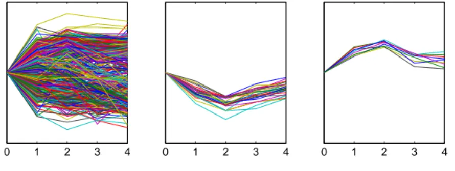
In a variety of fields, such as biology, economy or social sciences, time series are necessary to express characteristic features of underlying processes over time. For example, in the analysis of microarray gene expression data, the clustering of time series is an important objective in order to identify subsets of genes sharing a temporal expression pattern (see Figure 1.1).

According to Ernst et al. ([Erns 05]), more than 80% of the time series in the Stanford Microarray Database consist of the values measured at eight time points or less. That leads to a large number of data in a low-dimensional space ([Spri 11]).

Since most methods for analyzing long time series are not well-suited or not even applicable for short time series, different approaches and algorithms have to be developed. Many established methods for the analysis of short time series consider the behavior of biological data only in the phase of the modeling of cluster prototypes. In [Spri 11], Springer, Ickstadt and St¨ockler proposed a new method based on the minimization of the non-convex functional

F

(Θ, Y ) = d

m

TFP(Θ) + α m + 1 −

m

X

ℓ=1

j=1,...,N

max h y

, θ

i

!

, (1.1)

which also takes the actual (normalized) data Y = { y

}

into account. It combines the

“Total Frame Potential” (TFP) from [Bene 03] with a data-dependent penalty term. This technique of obtaining a tradeoff between regularization and minimizing cost imposed by a loss function is common in Statistics and Machine Learning Theory.

In this thesis, we analyze this functional on a mathematical basis, including an introduction

0 1 2 3 4 0 1 2 3 4 0 1 2 3 4

Figure 1.1: Sample data (left) and two groups of included short time series sharing similar expression patterns (middle and right)

into the necessary framework, and discuss the position of our method in the family of cluster algorithms as well as the relation of the inherent optimization to other problems in learning theory. Our central Theorem (Theorem 4.8) shows that for a positive regularization parameter α the minimizing family θ

, . . . , θ

of vectors on the unit sphere cannot be located on the spherical boundaries of the data-generated Dirichlet cells

D

= { v ∈ R

: k v k

= 1, h y

, v i = max

k=1,...,N

h y

, v i} .

Then it follows immediately that for each θ

there exists a unique y

such that

j=1,...,N

max h y

, θ

i =

y

, θ

holds in (1.1). This feature is the basis for a proposal of a group of related minimization problems which lead to further features of minimizers of the stated functional.

The outline is as follows. In Chapter 2, we introduce the basic theory of frames including the re- cent development on finite frames. We cite major results by Benedetto and Fickus ([Bene 03]) and Goyal et al. ([Goya 98]). The Total Frame Potential from [Bene 03] is considered from a linear algebra perspective and as an optimization problem with quadratic constraints us- ing Lagrange multipliers. As will be shown, the objective function can be formulated in the eigenvalues of a Gramian matrix leading to a polynomial problem of total degree four. Fur- thermore, we extend existing results on the minimizers of the TFP to all extrema and show that every local maximum is also global (Theorem 2.14).

Chapter 3 gives a short overview on cluster algorithms in general. The focus lies on the so-

called STEM algorithm by Ernst et al. ([Erns 05]), which contains connections to optimization

on unit spheres. Furthermore, a brief discussion on an inherent relation to classical problems by Tammes ([Tamm 30]) and Thomson ([Thom 04]) arising in biology and physics, respectively, is included. The basic idea is to generalize an approach by Benedetto, Czaja and Ehler from [Bene 10] in order to motivate the construction of the Penalized Frame Potential as a data-dependent version of the TFP whose minimizers serve as cluster centers (prototypes).

In Chapter 4 we analyze the behavior of the Penalized Frame Potential and extract simple characteristic features. Moreover, we characterize the minimizers in terms of Dirichlet cells of a certain subfamily of the underlying data on a unit sphere. This leads us to introduce mild relaxations of the given optimization problem in Chapter 5. We consider the minimization problem from the perspective of nonlinear optimization using the primal and their Lagrangian dual problems. For example, the optimization problem

(P2 ∗ )



 

  min

T∈R^d×m

k T

T k

+ α k T − Y

k

s.t. trace (T

T ) = m .

constitutes a mild relaxation where the primal objective function and the corresponding dual are equal in their respective optimal values, i.e. (P2 ∗ ) does not possess a duality gap. In this context, tools from matrix analysis such as the Wielandt-Hoffman-Theorem for singular values will be introduced. We also discuss the relation to other optimization problems in the field of Compressive Sensing and formulate a heuristic method based on the relaxations for computing minimizers of the PFP.

Chapter 6 evaluates the performance of the proposed method compared to standard cluster algorithms such as STEM ([Erns 05]), DIB-C ([Kim 07]) and the well-known k-means algo- rithm. For the evaluation, simulated and real data from biological experiments will be used.

Necessary tools for the evaluation such as permutation-based significance testing or the Ad-

justed Rand Index are introduced. We further present an example showing the applicability

of our PFP-based algorithm in feature recognition in multispectral data. Finally, Chapter 7

serves as a brief overview on open problems which will be dealt with in future work.

Chapter 2

Frames

Frames were first introduced in 1952 by Duffin and Schaeffer in their work on non-harmonic Fourier series ([Duff 52]). Later, during the rise of wavelets and the corresponding applications in Signal Processing Theory, they drew attention due to ground-breaking works like the ones by Daubechies ([Daub 92]), Chui ([Chui 92]) or Hern´andez and Weiss ([Hern 96]).

The reason for the increased interest in frames in signal processing is mainly based on their ability in extracting and stressing characteristic features from signals compared to using stan- dard orthonormal decompositions, e.g. wavelet bases. In contrast to bases, frames can be linearly dependent. The inherent redundancy leads to decompositions that are more stable against errors by corrupted or missing coefficients. A summary on the developments in frame theory and an overview on certain special cases can be found in the articles by Kovaˇcevi´c and Chebira ([Kova 07a, Kova 07b]).

Finite Unit Norm Tight Frames (FUNTFs) started attracting interest in the end of the 1990’s

and the beginning of the following decade due to publications by Goyal et al. ([Goya 98,

Goya 01]) or Benedetto and Fickus ([Bene 03]). Goyal et al. ([Goya 98]) proved that randomly

distributing m points independently and identically with a uniform distribution on the unit

sphere asymptotically leads to FUNTFs as m → ∞ . In 2003, Benedetto and Fickus ([Bene 03])

characterized the class of FUNTFs as vectors in K

which are exactly the minimizers of the

(Total) Frame Potential, a functional that we introduce in Section 2.1. Minimization of the

frame potential corresponds to finding configurations of m unit norm vectors which are in

equilibrium under the underlying (frame) force. The article initiated a fast development in this area whereas one has to admit that the theory basically rests on simple linear algebra due to the finite dimensionality. As we will show in the following chapters, many results on finite frames can be re-formulated using the singular value decomposition which simplifies the proofs as well.

Another reason for the increased consideration of FUNTFs was, for example, the optimality of analysis and synthesis of data in terms of a general quantization model ([Goya 01]). Shortly after the article by Benedetto and Fickus, Casazza generalized the frame potential approach by introducing the weighted frame potential distributing m vectors in K

on arbitrary centered spheres with radii r

, . . . , r

([Casa 04]). Together, Casazza and Fickus extended the frame potential concept even further to fusion frames ([Casa 09]).

In the theory of Compressed Sensing, where one is often interested in finding spanning sys- tems in which the given data has a sparse coefficient representation, FUNTFs have also been studied ([Dono 06]). Ehler ([Ehle 12a]), Ehler and Okoudjou ([Ehle 12b]) created probabilistic versions of the frame potential, and Ehler and Galanis ([Ehle 11a]) showed their applicability in directional statistics. An exhaustive view on the recent development in the theory of finite frames is given by Casazza and Kutyniok in [Casa 13].

Later on, in Section 3.3, we adapt a functional proposed by Benedetto et al. in [Bene 10], by generating a weighted mean of the frame potential and a data-fitting term. This already lead us to introduce the Penalized Frame Potential in [Spri 11] for the selection of cluster prototypes, which we will analyze and discuss for both theoretical and practical purposes in this thesis.

The primal objective will consist of the clustering of real-valued data vectors projected onto the unit sphere. This modeling justifies the concentration on FUNTFs which will be regarded primarily throughout this thesis after a general introduction into frame theory.

Definition 2.1. Let H be a Hilbert space and I an index set. A family of vectors Θ = { θ

}

in H constitutes a frame, if constants 0 < A ≤ B exist, such that for all y ∈ H the frame condition

A k y k

≤ P

k∈I

|h y, θ

i|

≤ B k y k

(2.1)

holds. A and B denote the frame bounds.

In the case of equal frame bounds A = B, the family { θ

}

is called tight. Duffin and Schaeffer ([Duff 52]) defined frames for the Hilbert space H = L

([0, 1]). In wavelet theory and signal processing, most results are formulated for the space of square-integrable functions over the real line, i.e. H = L

( R ).

In general, a family { θ

}

forms by definition a Bessel sequence, if there exists a Bessel bound B > 0, such that the upper bound condition in (2.1) holds. It is easy to see that the corresponding operator

T

: H → ℓ

(I ) y 7→ ( h y, θ

i )

is bounded with k T

k ≤ √

B. In functional analysis, T

is often denoted as Bessel operator whereas the wavelet community commonly uses the terms analysis or decomposition operator.

The adjoint operator T is called synthesis or reconstruction operator and given by T : ℓ

(I ) → H

(c

)

7→ P

k∈I

c

θ

.

If the lower bound condition in (2.1) also applies, i.e. { θ

}

being a frame, the composition S = T T

: H → H defines the frame operator. Furthermore, S is self-adjoint, positive, invertible and the inverse S

becomes itself a frame operator with bounds 0 < B

≤ A

. The corresponding family { θ ˜

}

with ˜ θ

= S

θ

for all k ∈ I defines the canonical dual frame satisfying the identities

y = X

k∈I

h y, θ

i θ ˜

= X

k∈I

h y, θ ˜

i θ

(2.2)

with unconditional convergence of both series for all y ∈ H ([Chri 08], Theorem 5.1.7). Note that one is often interested in finding other dual frames with certain features that are generally not satisfied by the canonical dual. For example, if H = L

( R ), compactness of the support is a common objective.

In the case of A = B, i.e. { θ

}

constituting a tight frame, we have S = A · Id where Id denotes the identity on H . Hence, (2.2) reduces to

y = A

X

k∈I

h y, θ

i θ

∀ y ∈ H (2.3)

and the frame condition (2.1) becomes the Parseval-type identity A k y k

= X

k∈I

|h y, θ

i|

∀ y ∈ H .

If A = 1, the frame { θ

}

is also often referred to as a Parseval frame. By Casazza and Kovaˇcevi´c ([Casa 03]), the following theorem on Parseval frames is known as Naimark’s theo- rem in operator theory and was first published by Akhiezer and Glazman in [Akhi 66]. Later on, the theorem was rediscovered and reformulated in the frame theoretical framework by Han and Larson in [Han 00a].

Theorem 2.2 (Naimark [Akhi 66], Han and Larson [Han 00a]). The family { θ

}

con- stitutes a Parseval frame of the Hilbert space H if and only if there exists a Hilbert space H

⊇ H with orthonormal basis { ϕ

}

such that the orthogonal projection P : H

→ H satisfies P ϕ

= θ

for all k ∈ I.

Note that if the elements of a Parseval frame are unit vectors, i.e. k θ

k = 1 for k = 1, . . . , m, the family is an ONB of H and vice versa.

2.1 Finite Frames

Throughout the following chapters we will use the finite-dimensional Hilbert spaces H = K

( K = C or R ) and the index set I = { 1, . . . , m } where d, m ∈ N . Unless stated otherwise, k · k denotes the Euclidean norm induced by the inner product h x, y i = y

x where y

is the transposed complex conjugate of y ∈ K

. It is a well-known fact (and easy to verify) that the finite family Θ = { θ

}

is a frame of H if and only if it spans K

. Note that we use { } -braces both for sets and for families of vectors like in [Bene 03]. Families are allowed to contain multiplicities of single elements whereas sets are not. However, the meaning will become clear from the context.

With column vectors θ

∈ S

, where

S

= { v ∈ K

| k v k = 1 } (2.4) denotes the unit sphere in K

, the matrix

T = [θ

, . . . , θ

] ∈ K

(2.5)

2.1. FINITE FRAMES defines the Frame Matrix

S = T T

=

m

X

k=1

θ

θ

∈ K

and the Gramian Matrix

G = T

T = ( h θ

, θ

i )

∈ K

.

Obviously, since θ

∈ S

, the diagonal entries of G satisfy g

= 1. In the following, let ( S

)

= S

× . . . × S

denote the m-fold Cartesian product of the unit sphere.

Example 2.3. The simplest FUNTFs in R

are given by the real and imaginary parts of the m

complex roots of unity, e.g. for m = 3 we get the frame

Θ = n

(1, 0)

, ( − 1/2, √

3/2)

, ( − 1/2, − √

3/2)

o with corresponding Frame Matrix

S =











1 −

−

0

−





















1 0

−

−

−











= 3/2 I

where I

stands for the 2 × 2 identity matrix. Furthermore, the Gramian matrix is given by

G =























1 −

−

−

1 −

−

−

1





















 .

Remark 2.4. (1) Note that the real and imaginary parts of the roots of unity form Grass- mannian frames in R

: FUNTFs are called equiangular, if | h θ

, θ

i | = c for all 1 ≤ k < ℓ ≤ m and some constant c > 0, i.e. the non-diagonal entries of the Gramian G are equal in absolute value. In general, the maximal frame correlation defined by Strohmer and Heath in [Stro 03]

M (Θ) = max

1≤k<ℓ≤m

|h θ

, θ

i| (2.6) satisfies the lower bound condition

M (Θ) ≥ s

m − d

d(m − 1) (2.7)

for all families Θ ∈ ( S

)

. Grassmannian frames are defined as the minimizers of (2.6).

The right-hand side of (2.7) is a Welch bound ([Welc 74]). It constitutes a sharp bound since equality holds if and only if Θ is equiangular and tight ([Stro 03]). If furthermore all elements θ

are normalized, Θ is an optimal Grassmannian frame. The problem of finding or constructing equiangular frames is closely related to arranging m linear subspaces of dimension n < d in R

such that the angles between the normal vectors are as large as possible, a problem which has been addressed by Conway et al. in [Conw 96] as a minimization problem in the Grassmannian space

G (d, n) = n

U R

| dim(U ) = n o .

(2) The special class of harmonic frames is generated by taking d ≤ m rows of a discrete Fourier transform matrix M of size m × m and letting θ

, . . . , θ

∈ K

denote the columns of that matrix. It is easy to see that { θ

}

constitute an equal-norm Parseval frame for K

with k θ

k =

q

m

for k = 1, . . . , m and normalization by p

d

leads to a FUNTF. An example for a real-valued version of such a matrix of size 3 × 3 was constructed by Zimmermann ([Zimm 01]):

M =









 1/ √

2 1/ √

2 1/ √ 2 1 cos(

) cos(

) 0 sin(

) sin(

)











is already normalized appropriately and taking the last d = 2 rows implies that the frame in Example 2.3 also is harmonic. Note that in the case K = R the choice of the d rows is not arbitrary.

Hochwald et al. ([Hoch 00]) propose the usage of harmonic tight frames in antenna array design which, interestingly enough, is again closely related to packings in Grassmannian spaces. The article also states that the construction of harmonic tight frames has been used earlier by Balan or Daubechies without publication.

(3) Multiplication of the frame elements in Example 2.3 by √

A

= p

2/3 leads to the Parseval frame

Θ = ˜ n ( p

2/3, 0)

, ( − 1/ √ 6, 1/ √

2)

, ( − 1/ √

6, − 1/ √ 2)

o

.

2.1. FINITE FRAMES

−1

−0.5 0

0.5 1

−1

−0.5 0 0.5 1 0 0.2 0.4 0.6 0.8 1

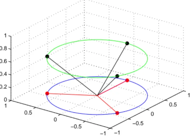
Figure 2.1: Example for Naimark’s Theorem from Remark 2.4.3 with a Parseval frame for R

(red) being the orthogonal projection of an orthonormal basis in R

(black)

Identifying H = R

with the (x, y)-plane in H

= R

and letting P : H

→ H the orthogonal projection, the family { ϕ

, ϕ

, ϕ

} with

ϕ

=









 p 2/3

0 1/ √

3











, ϕ

=











− 1/ √ 6 1/ √

2 1/ √

3











, ϕ

=











− 1/ √ 6

− 1/ √ 2 1/ √

3











is an orthonormal basis of R

and satisfies P ϕ

= θ

for k = 1, 2, 3 in the sense of Naimark’s Theorem (Theorem 2.2). Figure 2.1 presents the ONB consisting of ϕ

, ϕ

, ϕ

∈ R

and the corresponding vectors θ

, θ

, θ

∈ R

which constitute a Parseval frame. △

Example 2.3 underlines the following important property of FUNTFs:

Lemma 2.5 ([Goya 98]). Let Θ = { θ

}

∈ ( S

)

be a family of m ≥ d unit vectors.

Θ is an A-FUNTF, if and only if S = AI

∈ K

and A = m/d.

The value m/d is often referred to as the measure of redundancy of the frame. Whereas all orthonormal bases Θ ∈ in K

have A = 1, an increase of A shows the additional computational cost as well as redundancy in the information contained in representation (2.3).

Probably the most important characterization of FUNTFs for given dimension d and cardinal-

ity m was developed by Benedetto and Fickus in [Bene 03]. The idea is to define a repelling

force between the frame elements leading to an equilibrium.

Definition 2.6 ([Bene 03]). For a family Θ = { θ

}

∈ ( S

)

, the (Total) Frame Potential is defined as the mapping TFP : ( S

)

→ R ,

TFP (Θ) =

m

X

k,ℓ=1

|h θ

, θ

i|

.

Using the above notations, the TFP can be calculated by TFP (Θ) = k G k

= trace

(T

T )

= k S k

with k . k

denoting the Frobenius norm on K

. Moreover, if T = U ΣV

denotes the singular value decomposition (SVD) of T , where U ∈ U (d), V ∈ U (m) are unitary matrices and Σ = diag(σ

, . . . , σ

) ∈ R

with singular values σ

≥ 0 for all j, the frame potential reads as

TFP(Θ) = k Σ

Σ k

=

min{d,m}

X

j=1

σ

.

Furthermore, the constraint that the trace of the Gramian G equals the cardinality of the family Θ can also be formulated in terms of the SVD by

m =

m

X

k=1

k θ

k

= k T k

= k Σ k

=

min{d,m}

X

j=1

σ

.

Hence, using this relaxation, the TFP can be considered as a quartic polynomial under quadratic constraints. It is easy to see that the TFP under the given constraint is minimized by σ

= . . . = σ

= p

m/d if m ≥ d and σ

= . . . = σ

= 1 otherwise.

According to the following theorem, FUNTFs can be regarded as generalizations of the or- thonormal sequences in K

. It also connects the frame potential to the FUNTFs and orthonor- mal sequences, respectively.

Theorem 2.7 (Theorem 7.1 in [Bene 03]).

(i) Every local minimizer of TFP is also a global minimizer.

(ii) If m ≤ d, then

Θ∈(

min

TFP (Θ) = m (2.8)

and the minimizers are the orthonormal m-sets in K

, i.e. h θ

, θ

i = δ

for all k, ℓ =

1, . . . , m.

2.2. CRITICAL POINTS OF THE FRAME POTENTIAL (iii) If m > d, then

min

Θ∈(S^d−1)^m

TFP (Θ) = m

/d (2.9) and the minimizing families with m elements are the (m/d)-FUNTFs in K

.

Note that for the FUNTF Θ in example 2.3 we have

TFP (Θ) = 9/2 (2.10)

and the singular values satisfy σ

= σ

= p 3/2.

A method for generating FUNTFs { θ

}

in R

for m ≥ d can be derived from Casazza’s and Leon’s algorithm in [Casa 02a] and [Casa 02b]. The main idea here is to construct the orthogonal matrix V ∈ O(m) such that for V

= [v

, . . . , v

] it holds that k ˜ v

k = . . . = k v ˜

k = p

d/m, where ˜ v

= (v

, . . . , v

)

for k = 1, . . . , m are generated by omitting the last m − d rows of V

. Using U ∈ O(d) and Σ = diag( p

m/d, . . . , p

m/d) ∈ R

it follows that T = U ΣV

has unit vectors as columns and satisfies the constraints for the singular values for minima of the frame potential.

Remark 2.8. (1) In [Casa 04], Casazza et al. gave an alternative proof for Theorem 2.7, by formulating a generalization for the eigenspaces of the frame operator S. We will adapt this concept in the following section for a characterization of all critical points of the frame potential.

(2) Goyal et al. define in [Goya 01] the equivalence relation

T

∼ T

⇔ ∃ U ∈ U (d), ∆ = diag(δ

, . . . , δ

), δ

= ± 1 : T

= ∆U T

,

where U (d) is the group of unitary matrices in C

. If m = d + 1, all FUNTFs are in the same equivalence class. For example, the frame from example 2.3 is a representative of the

class containing all other FUNTFs with three elements. △

2.2 Critical Points of the Frame Potential

In the following, Θ denotes the family of unit norm vectors θ

, . . . , θ

and we concentrate on

the case K = R since it is quite illuminating. According to [Bene 03] and [Absi 08], we apply

the following definition:

Definition 2.9. The finite family Θ = { θ

}

∈ ( S

)

is called (TFP-)critical, if all θ

for k = 1, . . . , m are eigenvectors of the corresponding frame matrix S = T T

. In addition, if Θ is critical, we also call T = [θ

, . . . , θ

] critical. In the case, that a critical Θ is neither a local minimizer nor a local maximizer of TFP, Θ is called saddle point.

By Theorem 2.7, local minima of TFP are global. Furthermore, min

TFP(Θ) = m · max { 1, m/d } .

Applying the classical Lagrange approach for constrained minimization of the Frame Potential on the m-fold unit sphere in R

gives the Lagrange function

L (Θ, λ) = TFP(Θ) +

m

X

j=1

λ

k θ

k

− 1

=

m

X

k,ℓ=1

|h θ

, θ

i|

+

m

X

j=1

λ

k θ

k

− 1 where k · k is the euclidean norm. The m equality constraints

g

(Θ) = k θ

k

− 1, j = 1, . . . , m, describe the non-convex feasible set

( S

)

= S

× . . . × S

= { Θ | g

(Θ) = 0, j = 1, . . . , m } .

Since the Jacobian matrix of the mapping F : R

→ R

, F(Θ) = (g

(Θ), . . . , g

(Θ))

is

DF (Θ) =















 2θ

2θ

. ..

2θ

















∈ R

,

the full rank condition rank(DF )(Θ) = m is satisfied for all Θ ∈ ( S

)

, which is necessary for the application of the Lagrange approach to the problem at hand, see e.g. [Rock 93].

For the derivative of the TFP let j ∈ { 1, . . . , m } and θ

, . . . , θ

, θ

, . . . , θ

∈ S

. Define the functions h

: R

→ R by

h

(θ) = X

k,ℓ6=j

h θ

, θ

i

+ 2 X

k6=j

h θ

, θ i

+ h θ, θ i

.

2.2. CRITICAL POINTS OF THE FRAME POTENTIAL Then, h

is a quartic polynomial in the components of θ and the total derivative in θ is

∇ h

(θ) = 4 X

k6=j

h θ

, θ i θ

+ 4 h θ, θ i θ

which, with θ = θ

, leads to

∇ h

(θ

) = 4

m

X

k=1

h θ

, θ

i θ

,

or, equivalently,

∇ h

(θ

)

= 4Sθ

. Therefore it holds that

∇ TFP(Θ)

= 4 ST . (2.11)

Analogously, the total derivative of L in Θ and λ leads to the system of extremal conditions































4Sθ

+ 2λ

θ

.. . 4Sθ

+ 2λ

θ

k θ

k

− 1 .. . k θ

k

− 1































= 0

∈ R

,

or, with Λ = diag(λ

, . . . , λ

) denoting the diagonal matrix containing the Lagrange multi- pliers,

4ST + 2T Λ = 0 ∈ R

, (2.12)

k θ

k

= 1, j = 1, . . . , m .

Note that (2.12) is equivalent to Sθ

= −

θ

, k = 1, . . . , m. This implies that the Lagrange multipliers λ

, . . . , λ

satisfy an eigenvalue equation and by denoting the spectrum of S by spec(S) we have {− λ

/2, . . . , − λ

/2 } ⊆ spec(S). Hence, ( −

, θ

) are eigenpairs of S and only critical Θ are candidates for extrema of TFP.

Since every FUNTF Θ satisfies S =

I

, it follows from Eig(S, m/d) = R

that Θ is critical.

However, Benedetto and Fickus show in [Bene 03] that critical Θ exist which do not constitute

a FUNTF:

Example 2.10 ([Bene 03]). Let N = { ν

, . . . , ν

] ∈ R

with

ν

=















 1 0 0 0















 , ν

=

















− 1/2

√ 3/2 0 0















 , ν

=

















− 1/2

− √ 3/2 0 0















 , ν

=















 0 0 1 0















 , ν

=















 0 0 0 1















 .

Then the frame matrix S

is given by

S

=

















3/2 0 0 0

0 3/2 0 0

0 0 1 0

0 0 0 1

















and it is easy to see that ν

, ν

, ν

∈ Eig(S, 3/2) and ν

, ν

∈ Eig(S, 1).

Theorem 2.11 ([Bene 03]). A finite sequence of unit vectors Θ = { θ

}

is critical if and only if the sequence may be partitioned into a collection of mutually orthogonal vectors, each of which is a FUNTF for its span. Furthermore, the partition may be chosen explicitly to be { E

} where E

= { θ

: Sθ

= µθ

} . Also, the frame constant of E

is µ, and the spans of the { E

} are precisely the non-trivial eigenspaces of S.

Consider µ

> µ

> . . . > µ

≥ 0 as the pairwise distinct eigenvalues of S. Analogously to the proof of Theorem 7.4 in [Bene 03] we define for j = 1, . . . , s the index sets

I

= { k ∈ { 1, . . . , m } : Sθ

= µ

θ

} ,

which build a partition of { 1, . . . , m } (with I

= ∅ , if S is not regular, i.e. µ

= 0). By Theorem 2.11, the families { θ

}

build frames of the eigenspaces if Θ is critical. Due to the symmetry of S and the orthogonality of the eigenspaces in that case, the map TFP can be decomposed into the restrictions on its eigenspaces:

TFP(Θ) =

m

X

k,ℓ=1

|h θ

, θ

i|

=

s

X

j=1

X

k,ℓ∈Ij

|h θ

, θ

i|

=:

s

X

j=1

TFP

(Θ) .

Using the notations m

= | I

| and d

= dim Eig(S, µ

), Theorem 2.11 immediately leads to

the following conclusion.

2.2. CRITICAL POINTS OF THE FRAME POTENTIAL Corollary 2.12. If Θ is critical, the restrictions on the eigenspaces of S satisfy

TFP

(Θ) = X

k,ℓ∈Ij

|h θ

, θ

i|

= µ

m

, j = 1, . . . , s . Furthermore, µ

= 1 if { θ

}

is ONB of Eig(S, µ

) and µ

=

j

if the family is a frame.

Proof. Theorem 2.11 shows that TFP

(Θ) = m

= d

if { θ

}

is an ONB of Eig(S, µ

) and TFP

(Θ) =

2 j

dj

if it is a FUNTF. Then for v ∈ Eig(S, µ

) it follows that µ

v = Sv =

m

X

k=1

h v, θ

i θ

= X

k∈Ij

h v, θ

i θ

which is v in the case of an ONB or

j

v otherwise.

The matrix S = T T

with T = [θ

, . . . , θ

] has only non-negative eigenvalues due to positive semi-definiteness. Since it holds that

k Sθ

k

= k

m

X

ℓ=1

h θ

, θ

i θ

k

= k θ

+ X

ℓ6=k

h θ

, θ

i θ

k

= k θ

k

+ 2 Re h θ

, X

ℓ6=k

h θ

, θ

i θ

i + k X

ℓ6=k

h θ

, θ

i θ

k

= 1 + 2 X

ℓ6=k

|h θ

, θ

i|

+ k X

ℓ6=k

h θ

, θ

i θ

k

≥ 1 , (2.13) the (normalized) column vectors of critical T are eigenvectors of S with eigenvalues greater or equal 1. Moreover, equality holds if and only if θ

⊥ span { θ

, . . . , θ

, θ

, . . . , θ

} .

Lemma 2.13. If Θ is critical, then spec(S) ⊂ ( { 0 } ∪ [1, m]) and the Lagrange multipliers satisfy − 2m ≤ λ

≤ − 2, k = 1, . . . , m.

Proof. For the verification of the upper bound consider the singular value decomposition T = U ΣV

. As seen before

m =

d

X

j=1

σ

,

with σ

being the eigenvalues of S. If an eigenpair (µ, v) with v / ∈ span { θ

, . . . , θ

} exists,

it follows that µ = 0 since R

= span { θ

, . . . , θ

} ⊕ ker(S) is an orthogonal sum. Together

with (2.13) it can be concluded that spec(S) is in { 0 } ∪ [1, m]. Finally, the extremal condition Sθ

= −

θ

gives 1 ≤ −

≤ m for all k = 1, . . . , m which completes the proof.

In [Bene 03], Benedetto and Fickus consider only minima of the frame potential for the char- acterization of the FUNTFs. From

TFP(Θ) =

m

X

k,ℓ=1

|h θ

, θ

i|

≤

m

X

k,ℓ=1

k θ

k

k θ

k

= m

,

we also get that Θ is a global maximum of the function TFP if and only if c

, . . . , c

∈ C exist with | c

| = 1 and c

θ

= . . . = c

θ

. In that case the entries of the Gramian matrix satisfy

| g

| = 1. Thus, in R

, these are exactly the subsets of the unit sphere consisting of antipodal vectors. The following theorem states that also every local maximum of TFP is global.

Theorem 2.14. Let m, d ∈ N and µ

, . . . , µ

∈ { 0 } ∪ [1, m] with µ

> µ

> . . . > µ

≥ 0 denoting the pairwise distinct eigenvalues of S. The critical family Θ = { θ

}

is a saddle point of TFP, if and only if one of the following holds:

(i) µ

≥ 1,

(ii) µ

= 0 and the multiplicity d

of µ

satisfies 1 < d

< min { d, m } .

Proof. A local and global minimum can be ruled out by Theorem 2.7, since these do only have the (min { d, m } )-fold eigenvalue µ

= max { 1, m/d } . Hence, it suffices to show that no local maximum can exist under the assumptions.

By Corollary 2.12, the restrictions on the eigenspaces take their global minima in Θ:

TFP

(Θ) = X

k,ℓ∈Ij

|h θ

, θ

i|

= µ

| I

| , j = 1, . . . , s.

If µ

≥ 1, it holds that µ

> 1 and the family { θ

}

therefore is a FUNTF of Eig(S, µ

) by Theorem 2.11. Thus, a small perturbation on θ

, k

∈ I

, in Eig(S, µ

), such that the FUNTF-condition is not satisfied, enlarges the function value of TFP

and the function value of TFP = P

j=1

TFP

increases in the corresponding direction. If µ

= 0 ∈ spec(S), almost

the same argument can be used. In that case, R

= Eig(S, µ

) ⊕ Ker(S) is an orthogonal

sum where dim Ker(S) > 0. Since Θ is critical, the family { θ

}

builds a FUNTF or

2.2. CRITICAL POINTS OF THE FRAME POTENTIAL orthonormal system of Eig(S, µ

). If dim Eig(S, µ

) > 1, perturbations on θ

in Eig(S, µ

) revoke the minimality condition which, again, is equivalent to the existence of an ascend direction in Θ.

The only case which is open is µ

= 0 and d

= 1. In that case it holds that TFP(Θ) = m

, which corresponds to a global maximum. The equivalence follows directly from the fact, that no other cases are possible.

The only case which has not been regarded in the proof is µ

= 0 and dim Eig(S, µ

) = 1 which is only possible if rank(T ) = dim span { (θ

, . . . , θ

) } = 1. In that case Θ is critical with the single positive eigenvalue µ

= m of S.

Corollary 2.15. Let Θ be a critical family. Then Θ is a global maximum, if and only if µ

= 0 and µ

= m is an eigenvalue of S with multiplicity 1.

If two distinct eigenvalues µ

> µ

> 1 of S exist, directions of increase or decrease of the TFP can be constructed directly with the method of Benedetto and Fickus in the proof of Theorem 7.4 in [Bene 03]. The vectors θ

, k ∈ I

, are a frame of Eig(S, µ

). Due to the linear dependence, there exist β

∈ C , k ∈ I

, satisfying P

k∈I2

β

θ

= 0. Without any restriction, β

can be chosen such that | β

|

< 1/2. Let ε > 0, (µ

, θ) eigenpair with normalized θ and Θ = ˜ { θ ˜

}

with

θ ˜

=







p 1 − ε

| β

|

θ

+ εβ

θ, k ∈ I

θ

, k / ∈ I

.

Then

TFP( ˜ Θ) = TFP(Θ) + 2(µ

− µ

)ε



 X

k∈I2

| β

|



 + R(ε)ε

, where R(ε) is bounded in magnitude and therefore TFP( ˜ Θ) > TFP(Θ).

Thus, the restriction µ

> 1 guarantees the existence of the linear coefficients β

as described.

For µ

= 1 the construction from the proof of Theorem 2.14 can be used. On the other hand,

we receive a decrease in function value, if instead of the elements in Eig(S, µ

) the elements

of the spanning frame of Eig(S, µ

) are altered by the construction by Benedetto and Fickus.

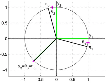
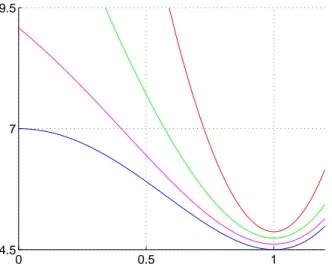
Example 2.16. Let N = (ν

, . . . , ν

) be defined as in Example 2.10. Then

S =

















3/2 0 0 0

0 3/2 0 0

0 0 1 0

0 0 0 1

















and TFP(N ) = k S k

= 13/2.

The vectors ν

, ν

, ν

constitute a FUNTF of Eig(S, 3/2) and ν

, ν

are ONB of Eig(S, 1).

Hence, N is critical and the partition of the index set { 1, . . . , 5 } according to the proof of Theorem 2.14 is I

= { 1, 2, 3 } and I

= { 4, 5 } . For β

= β

= β

=: β ∈ R we get P

k∈I1

βν

= 0. Let γ := ε | β | and define according to the construction ˆ ν

= ν

, ν ˆ

= ν

and

ˆ

ν

= p

1 − γ















 1 0 0 0















 +















 0 0 γ 0

















=

















p 1 − γ

0 γ 0















 ,

ˆ

ν

= 1 2

















− p 1 − γ

p 3 − 3γ

2γ 0















 ,

ˆ

ν

= 1 2

















− p 1 − γ

− p

3 − 3γ

2γ

0















 .

Then the new frame matrix S ˆ = ˆ T T ˆ

is S ˆ = diag

3

2 (1 − γ

), 3

2 (1 − γ

), 3γ

+ 1, 1

and therefore

TFP( ˆ N ) = k S ˆ k

=

(1 − γ

)

+ (3γ

+ 1)

+ 1

=

+

γ

− 3γ

= TFP(N ) + g(γ) with g(γ) :=

γ

− 3γ

< 0 for 0 < γ < √

2/3 and g strictly decreasing on [0, 1/3]. For

γ = 1/3 we have S ˆ = diag(

,

,

, 1). Furthermore, { ν ˆ

, . . . , ν ˆ

} constitutes a FUNTF of

Eig(S, 4/3) and ν ˆ

is ONB of Eig(S, 1).

2.3. SPECTRUM AND NON-TIGHTNESS

2.3 Spectrum and Non-Tightness

In this last section on the introduction of Frames, we define the Non-Tightness as a means in order to measure “how far away” from a FUNTF a family of vectors in S

is.

Definition 2.17. Let m ≥ d, Θ = { θ

}

⊂ S

be a finite family of (not necessarily pairwise distinct) normalized vectors, T = [θ

, . . . , θ

] ∈ C

and S = T T

. Then the mapping NT : S

× . . . × S

→ R ,

NT(Θ) =

S − m

d I

2 F

defines the Non-Tightness of the family Θ.

Obviously, the Non-Tightness is closely connected to the frame potential which satisfies TFP(Θ) = k S k

. However, as we will see in Chapter 4, the Non-Tightness works as a helpful tool in the analysis of the asymptotic behavior of certain functionals used for the data clustering approach, which we introduce in Chapter 3.

It is easy to see from (2.1) that the eigenvalues µ

= σ

of an arbitrary frame operator are located in the interval [A, B] where 0 < A ≤ B < ∞ , which already implies the regularity of S. As stated in Lemma 2.5, if the columns of T constitute a FUNTF, then A = B = m/d. Let T = U ΣV

be again the singular value decomposition of T with Σ = diag(σ

, . . . , σ

) ∈ R

and unitary matrices U ∈ U (d) and V ∈ U (m). By definition, NT is zero if and only if Θ is a FUNTF. Furthermore, by the symmetry of S, NT can be written as TFP − m

/d since

NT(Θ) = trace

(S − m d I

)

= k S k

− 2m

d trace (T T

) + m

d

trace (I

)

= TFP(Θ) − m

d .

The following proposition shows that the Non-Tightness has a natural interpretation as the variance of the spectrum of the frame matrix S.

Proposition 2.18. Let µ

≥ µ

≥ . . . ≥ µ

≥ 0 denote the eigenvalues of the frame matrix S. Then µ ¯ =

is the mean of the eigenvalues and the sample variance σ ˆ

satisfies

(d − 1)ˆ σ

= NT(Θ) . (2.14)

Proof. µ ¯ =

follows directly from the fact that m =

d

X

j=1

σ

=

d

X

j=1

µ

.

Then, due to the unitary invariance of the Frobenius norm,

NT(Θ) =

S − m

d I

2 F

=

diag(σ

, . . . , σ

) − m d I

2 F

=

d

X

j=1

(µ

− µ) ¯

which establishes (2.14).

Chapter 3

Cluster Algorithms for Short Time Series

Clustering real data describes the attempt to identify groups whose members are similar in terms of a predefined measure. This rather old problem affects many fields in science and a vast number of approaches exist in the literature. Nowadays, the clustering prob- lem is commonly dealt with in Data Mining and Machine Learning Theory. A classification of different cluster algorithms into five major categories can be found, e.g., in the book of Han and Kamber ([Han 00b]). Based on this classification, various examples for partitioning (e.g. k-means, k-medoids, fuzzy c-means), hierarchical (agglomerative/ bottom-up, divisive/

top-down), density-based (DBSCAN, OPTICS), grid-based (STING) and model-based (Auto- Class, ART) methods are described in Liao’s exhaustive survey ([Liao 05]), where the problem of choosing appropriate distance or dissimilarity measures for the clustering process is also ad- dressed.

The major part of the following chapter has already been published in [Spri 11]. However, the analysis and the evaluation including numerical results, which follow in Chapters 4, 5 and 6, have not been included in the mentioned contribution.

Classical methods for the analysis of long time series are based on principal component analysis

and discrete wavelet transforms ([Hast 01], [Qu 03]). A feature-based incremental clustering

method is described by Vlachos et al. ([Vlac 03]) where the multilevel resolution capability of Haar wavelets is combined with a coarse-to-fine selection of centers for the k-means clustering algorithm. More recently, dimension reduction methods by kernel eigenmap methods like Laplacian ([Belk 03], [Ehle 11b]) and Schroedinger eigenmaps ([Czaj 13]) project the data into lower-dimensional subspaces with as little distortion as possible. In contrast, in most cases of microarray analysis, the lengths of the time series are rather small. For example, according to Ernst et al. ([Erns 05]), more than 80% of the time series in the Stanford Microarray Database (http://smd.princeton.edu, accessed November 28, 2013) consist of the values measured at eight time points or less. That leads to a large number of data in a low-dimensional space.

Since most methods for analyzing long time series are not well-suited or even applicable for short time series, different approaches and algorithms have to be developed.

In some applications, data-dependent frames are computed in order to generate sparse co- efficient representations of the given data. The advantage rests on the fact that frames as redundant spanning systems – sometimes also denoted as overcomplete dictionaries – allow for different choices of these representations. In the clustering problem for short time series we deal with the problem of determining cluster prototypes. These prototypes are in a sense also supposed to represent the expansion of the data, which is why we propose a frame theoretic approach in this thesis.

Prototype selection is typical in partitioning methods. Approaches for the application on data from short time series include the Short Time Series Expression Miner (STEM) developed by Ernst et al. ([Erns 05]) and Difference-Based Clustering (DIB-C) by Kim and Kim ([Kim 07]).

In the following, we primarily concentrate on the STEM algorithm.

The first step of the STEM approach consists in constructing model profiles (cluster specific prototypes of time series) p

, . . . , p

such that

min

dis(p

, p

)

is maximized, where dis is an appropriate dissimilarity measure.

Section 3.1 gives a geometric interpretation of the dissimilarity measure in the STEM algo-

rithm, justifying the application of frame theoretic tools. Afterwards, in Section 3.2, we show

that the main problem in the STEM algorithm has a natural connection to some classical prob-