Temporal Activation Profiles of Gene Sets for the Analysis of Gene Expression Time Series
André König
Submitted to the Department of Statistics of the TU Dortmund University
in Fulfillment of the Requirements for the Degree of Doktor der Naturwissenschaften
Dortmund, November 2013
Referees:
Prof. Dr. Jörg Rahnenführer PD Dr. Marco Grzegorczyk
Date of Oral Examination: January 27, 2014
for my family
Acknowledgments
The last years passed like days, but now the work is done and my PhD thesis is ready for printing. Research is never done by one person alone. Hence, it is time to look back and analyze the history of this achievement.
First of all, I would like to express my deep gratitude to Prof. Dr. Jörg Rahnen- führer for the competent supervision of my work, for his open-mindedness, and for his infectious optimism, which was extremely encouraging in difficult times.
Furthermore, my thanks goes to my committee members Prof. Dr. Katja Ickstadt, PD Dr. Marco Grzegorczyk, and Dr. Adrian Wilk. Thank you for your time and effort.
My work benefited hugely from the excellent educational, administrative, struc- tural, and organizational support of the Graduate School of Statistical Modeling during my PhD time (special thanks Eva Brune and Prof. Dr. Joachim Kunert).
The very time consuming simulation studies had only be possible due to the neintim and LIDO computing clusters (Thanks to all contributors and Dr. Bernd Bischl for the introduction). Connected to the computational part, I would like to thank Michel Lang for the help with speeding up my R code by introducing me to C++ and Rcpp. Olaf Mersmann helped to speed up my work flow by suggesting the use of Emacs and helping with start-up difficulties. I would like to thank Sebastian Krey and JProf. Dr. Uwe Ligges for the fast and nerveracking (ad)ministration of the faculty’s electronic brain(s). Moreover, I am very grateful to Franziska Elze and Ilya Ivanov for the help within the jungle of the ArrayExpress data base.
In addition, I would like to thank all the as yet unmentioned colleagues at the faculty of statistics for their support and critical reflections.
My special thanks goes to my own social supporting system, which distracted my thoughts and helped me to complete my thesis without going crazy.
I owe all my thanks to my family, my parents for tracing the academic path and supporting me on my way so far and beyond, Peter for his fully grounded point of view and Steffen for his outstanding characteristic to put my ideas in question.
Finally, I want to thank my love Helena, who is always there for me; and my son
Darius for the enlightening example of apprehending the world from scratch.
1 Introduction to the Analysis of Gene Expression Time Series Data 7 2 Aspects of Analyzing Gene Expression Time Series Data on a Gene Set Level 9 2.1 Gene Expression Data Characteristics . . . . 10 2.2 Definitions of Gene Sets . . . . 17 2.3 Experimental Designs, References and Formalization . . . . 21 3 Methods for the Analysis of Gene Expression Time Series 25 3.1 Gene Set Testing Based on Differentially Expressed Genes . . . . . 27 3.2 Clustering Approaches . . . . 30 3.3 Other Approaches for the Gene Set Analysis of Gene Expression Time
Series . . . . 33 4 Estimating Temporal Activation Profiles of Gene Sets 35 4.1 Adapted Methods from GSA in Two-Condition Experiments . . . . 38 4.2 GSA-Type Algorithms for Determining Gene Set Activation Profiles 44 4.3 Smoothing of GSA-Type Gene Set Activation Profiles . . . . 50 4.4 Ranking of GSA-Type Gene Set Activation Profiles . . . . 56 4.5 Rotation-Test-Type Algorithm for Determining Gene Set Activation
Profiles . . . . 57 4.6 The Modified STEM Algorithm . . . . 60 4.7 The maSigFun Algorithm . . . . 63
5 Simulation Study 65
5.1 Short Characterization of the Four Recycled Example Data Sets . . 66
5.2 Construction of a Simulation Study by Recycling of Given Data . . 69
5.3 Simulation Study to Compare the Methods . . . . 85
5.4 Simulation Study to Evaluate the Smoothing Algorithms . . . 107
Simulation Study to Evaluate the Smoothing Algorithms . . . 107
5.5 Joint Conclusions from Both Simulation Studies . . . 133
6 Application of Gene Set Activation Profile Estimation 139 6.1 Filtering the Gene Universe . . . 139
6.2 Summary Over All Profile Algorithms and Data Sets . . . 144
6.3 Aldosterone Effect on Mouse Heart Gene Expression . . . 150
6.4 Embryonic Mouse Ovary Development Experiment . . . 154
6.5 Gene Expression During Wound Healing in Skin and Tongue . . . . 159
7 Discussion and Summary 173
List of Figures 197
List of Tables 205
A FDR q-value in the TS-ABH Procedure 209
B Figures and Tables 213
List of Symbols 281
Introduction to the Analysis of Gene Expression Time Series Data
In the second half of the 20
thcentury molecular genetics was established as a new field in biology. From the central dogma of molecular genetics first postulated by Francis Crick in 1958 it lasted another 37 years until the first genome of the bacterium Haemophilus influenzae was fully sequenced. This was only possible due to enormous scientific and technological advances like the discovery of the enzyme reverse transcriptase and the proceedings in automation and miniaturization with the PCR procedure as outstanding mile stone. In the decade around the turn of the millennium the advent of high throughput technologies allowed the parallel analysis of tens of thousands of genes or their transcripts with a single experiment on a chip smaller than a fingertip.
This thesis focuses on the analysis of the quantitative gene expression data
generated by high throughput time series experiments. The second chapter elucidates
the statistical challenges arising from the task to analyze an enormous number of
genes with a much smaller sample size for a few time points. Usually analyzing
gene sets instead of single genes supports the researcher at least in two ways. The
reduction of dimensionality in the data increases statistical power in the findings
of significant changes in gene expression and the a priori definition of gene sets in
the context of molecular functions or pathways facilitates the interpretation of the
findings. There are various methods available for the gene wise analysis of gene
expression time course experiments and gene set testing in the time series context.
The common approaches are discussed in the third chapter. On the other hand there is a lack of methods for estimating an activation profile of differential expression in the gene set setting, which is the overall objective of this thesis.
Three ways of estimating a group activation profile are introduced in the third
chapter. Each algorithm attempts to represent the differential expression of a
significant number of the included genes for a parallel consideration of a large number
of gene sets. Two standard algorithms from literature – STEM and maSigFun – are
presented for comparison purposes. The accuracy of the five approaches is compared
in an extensive simulation study in the fifth part of the thesis. A second large
simulation study in the same chapter evaluates smoothing procedures for the three
activation profile algorithms. The sixth chapter provides the application of the
activation profile estimation algorithm on four exemplary data sets and different
sources of gene set definition. In the last chapter the findings are summarized and
discussed.
Aspects of Analyzing Gene Expression Time Series Data on a Gene Set Level
Gene expression data confronts the statistician with the task of parallel analyzing tens of thousands features representing genes with only a few measurements. In the time course experimental design there are often only a few time points with non-uniform sampling scheme, which is an additional challenge for the researcher.
The first section in this chapter elucidates the type of data, which is considered
in this thesis; from the biological backgrounds to the symbolic notation used in
the following chapters. The second section provides an overview of the ideas and
sources of gene set definitions used for gene expression analysis. Currently available
methods for analyzing gene expression data resulting from a time course experiment
are shown in the third section of this chapter. It has to be noted that there currently
no methods are available that explicitly estimate temporal activation profiles of gene
sets, which is the objective of the thesis. Nevertheless the established algorithms
provide beneficial ideas, which can be modified to achieve an estimation procedure
as is demonstrated in chapter 4.
2.1 Gene Expression Data Characteristics
The Biological Background
All cellular components and functions of all living organisms depend directly or indirectly on molecules, called proteins. Proteins consist in their primary structure of one or more chains of aminoacids. The information about the order and type of the 20 different amino acids, which determines each protein is stored in the cells Deoxyribonucleic acid (DNA). In order to build a protein all organisms use a transcription of the double-stranded DNA into a single-stranded Ribonucleic acid (RNA) molecule, which codes the amino acid sequence forming the corresponding protein.
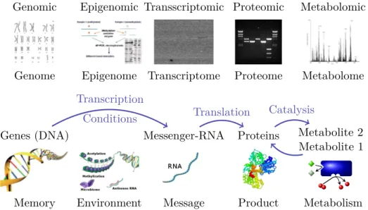
Gene expression data means measurements of the qualities and quantities of the cells RNA. Often these measurements are restricted to the messenger RNA, which is a replicate of the part of the genetic information coding for a single protein in the cells nucleus. Transcripts is a synonymously used term for RNA-strands and the whole space of transcripts is called transcriptome as can be seen in Figure 2.1 on the facing page, in which the main research areas related to bioinformatics are shown within their biological context.
High Throughput Technologies and Sources of Gene Expression Data
A number of high throughput technologies is available to generate gene expression data corresponding to thousands of transcripts from a small sample of cell plasma.
All manufacturers have in common, that they provide chips with an area of 1 - 2 cm
2, which contain a matrix of fixed oligonucleotides complementary to a priori chosen transcripts. A prepared cell medium containing the transcripts of interest in the current experiment is applied on this slide and the (labeled) fragments of the probe RNA hybridize complementary to the corresponding sites on the chip.
The measurement of transcript quantity is commonly derived of an optical signal
scanning the whole slide with a high resolution.
Memory Environment Message Product Metabolism Genes (DNA) Messenger-RNA Proteins Metabolite 2 Metabolite 1 Transcription
Conditions Translation Catalysis
Genome Epigenome Transcriptome Proteome Metabolome Genomic Epigenomic Transscriptomic Proteomic Metabolomic
Figure 2.1: Sketch of the main areas of bioinformatics (upper line) in combination with typical data, the term of the entirety of features (the omes), the biological interactions between the cells molecules and a more colloquial terminology lend from informatics.
The Gene Expression Omnibus (GEO, see Edgar, Domrachev, and Lash (2002)) is a data base for high-throughput functional genomic data and a free source of such data. The ArrayExpress data base (Parkinson, Kapushesky, et al. (2009)) is another repository for this type of data, but includes most of the GEO data sets.
Though there are other free online data bases for gene expression data, a view on the available technologies on ArrayExpress gives an impression about the distribution of the experiments on the different methods. Table 2.1 on the next page lists the number of experiments for the main high throughput technologies, which provide quantitative information about the presence of transcripts in a cell medium.
Miller and Tang (2009) briefly describe the available array technologies for gene
expression experiments. The microarray technologies (chip technologies from Ta-
ble 2.1) mainly differ in the way how to deposit the complementary oligonucleotides
on the chip surface. This can be done by printing copies of these base sequences
as a whole on the array (cDNA chip) or generate the sequence base by base with a
photolythographic procedure (Affymetrix, NimbleGen) or respectively by contactless
Table 2.1: Gene expression experiments found in the ArrayExpress repository grouped by technology and time series experiments. The numbers were obtained by queries in the ArrayExpress Browser on 1
stof November 2013. The overall used keyword was “RNA assay”. For the Time series value “ef:time” was used. For the microarray technologies the keyword by array was combined with the corresponding manufac- turer/chip name, i.e “NimbleGen”, “Agilent”, “Affymetrix”, “Illumina”, “cDNA”. The numbers for the other technologies are obtained by the keyword in the left column.
Manufacturer / Technology Data Sets Time Series cDNA arrays; spotted chips 2330 196
Roche NimbleGen chips 671 53
Agilent one color chips 3991 413
Affymetrix one color chips 17232 1652
Illumina Bead chips 2745 294
RT-PCR + RT-qPCR 915 62
sequencing assay 2924 183
printing (Agilent). Illumina bead arrays use beads with identical oligonucleotides on their surface, which randomly assort to the wells on the array. This necessitates an additional mapping step, which also serves as quality control. Another difference between the array technologies is the number of bases in the oligonucleotides fixed on the array beginning with 20 (Affymetrix) up to several hundreds (spotted arrays).
There is a trade-off between sensitivity and specificity related to the length of the sequence. Longer sequences provide higher sensitivity but lower specificity and vice versa (see Miller and Tang 2009, p. 612–614). In contrast to chip technologies the Real-time polymerase chain reaction (RT-PCR) techniques and the up-coming high-throughput sequencing methods (also known as “next generation sequencing”) give information about both the transcript quantity and sequence of the probes’
oligonucleotides. This allows to quantify even those transcripts, whose sequence was unknown or not yet considered in the expression experiments.
Essentially, all of the technologies shown in Table 2.1 are in principle suited to
be analyzed on a gene set level in time. Nevertheless this thesis focuses on the
Affymetrix technology due to the fact that microarrays of this manufacturer were
used for about two thirds of all gene expression time series experiments listed in the
ArrayExpress data base.
Affymetrix GeneChips
Dalma-Weiszhausz, Warrington, et al. (2006) provide a detailed description of the Affymetrix GeneChip technology and the corresponding experimental setup for measuring gene expression from cell RNA. A scheme of the Affymetrix microarray construction and a gene expression experiment is shown in Figure 2.2 on the following page. A transcript on Affymetrix microarrays is represented by a probe set of typically 11 oligonucleotides of 25 base pairs length. Each oligonucleotide appears twice on a chip; once with the real target sequence as perfect match (PM) probe and once as mismatch (MM) probe. The MM probe of the probe pair differs only by the 13
thbase from the PM probe and is included due to recognized signal from cross-hybridization, nonspecific binding or technical noise. A photolithographic process applies millions of identical oligonucleotide sequences onto an 11 µ m
2-sized feature space on the quartz chip surface corresponding to each probe sequence. The manufacturer Affymetrix sells gene expression arrays for many species with tens of thousands probe sets representing the exon regions (part of a gene sequence transcribed to RNA) of a priori known transcript-sequences.
In order to obtain the gene expression measurements, the RNA extracted from various cells must be amplified. The amplification is achieved by reverse transcrip- tion to cDNA, which is thereafter repeatedly transcribed to Biotin-labeled RNA.
After a fragmentation step the labeled short RNA-strands are applied onto the Affymetrix array, where the labeled RNA-strands complementary hybridize to their oligonucleotide counterparts. Non-binding and weakly binding RNA-oligonucleotides are washed out by a cleanup step. The Biotin-labeled bases are stained with a fluorescent-dye afterwards and after another cleanup step the hybridized chip is read out by a high definition laser scanner. Only those feature spaces with stained RNA on it send fluorescent light back to the sensor. The corresponding measured light intensity is a measure for the quantity of hybridized RNA and cell RNA, respectively.
RNA from different experimental conditions has to be examined on different chips
due to the array design. Furthermore, there are no replicates for the expression
probe sets on the array. Hence, replicates for the gene expression measurements
RNA Extraction
Reverse Transcription cDNA
Transcription to RNA and Biotin- labeling
B B
B B
B B
B B
B B
B B
Fragmentation
B B B B
B B B B
5’
3’
T A A T A G A C G G G G G A T C G G C G A C A T T C T
G T
... ...
T A A T A G A C G G G G G A T C G G C G A C A T T T A A T A G A C G G G G T A T C G G C G A C A T T Perfect Match Probe
Mismatch Probe
Hybridization
B B
B B
Cleanup, Staining, Cleanup
B B
B
Scanning
Figure 2.2: General construction of an Affymetrix gene expression microarray and
the experimental work flow to obtain quantitative data for the examined transcripts.
are only available, if multiple chips are hybridized under the same condition. The intensity values from the scanner are also called raw expression values and commonly stored in .cel files. These intensities are biased due to several reasons and hence have to be preprocessed before applying a differential expression analysis.
Data Preprocessing by Robust Multiarray Analysis
There are several preprocessing algorithms for microarrays proposed in the literature, which can be divided into the three steps: background correction, normalization across arrays and summarization of multiple probes per transcript target. Robust Multiarray Analysis (RMA) is an approach introduced by Irizarry, Bolstad, et al.
(2003), which accomplishes these three preprocessing steps.
Optical noise and non-specific binding to the oligonucleotides on the array lead to an unspecific background signal even for absent target transcripts and make a corresponding correction necessary. Z. Wu, Irizarry, et al. (2004) refine the background model of RMA in the sense, that the different binding affinity of the four nucleotide bases is taken into account for the estimation of unspecific binding.
The empirical Bayes version of their GC-RMA algorithm is applied as background correction to the raw gene expression data in this thesis.
Each array is processed under individual conditions, which may also include individually prepared RNA samples from different laboratories and read by different Scanners. Those conditions may affect the measured intensities, but do not provide information about the (differential) transcript expression. Therefore, a normalization step is needed to make the expression values comparable across all arrays hybridized in the study. RMA uses quantile normalization to unify the distribution of the probe values across all arrays.
In the Affymetrix array design multiple probes in one probe set quantify the same
transcript. The different loci on the sequence and the varying sequence-dependent
binding affinity of the probes may lead to a significant variation in the signal strength
among the probes within a probe set. A robust summary resistant to outliers is
needed in order to combine the probe set intensities to obtain a reliable expression
value for the whole transcript. Tukey’s median polish procedure is applied by
RMA to estimate the probe set expression value, which is synonymously denoted as transcript or gene expression value in the following.
Time Series Gene Expression Data
Gene expression time series experiments provide insight into the molecular biology
processes inside an organism over time. Usually time series experiments focus on the
changing transcription after suspending a stress condition (e.g. starvation or a drug)
or on the gene activation during a natural process (e.g. embryonic development of a
certain organ). The analysis is challenging due to the biological variability between
the examined individuals and even between cells of the same individual, which
may have different stages in their cell cycles. The analysis is further complicated
by the circumstance that most experiments cover only a few time points, which
are often not uniformly sampled. In contrast to static experiments the number
of biological or technical replicates at the same time point is very restricted as
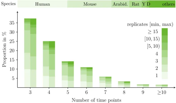
illustrated in Figure 2.3. Since the collection of gene expression data comes along
with the destructive testing of several cells no real longitudinal data is available
even if the same individuals are tracked across time. All in all the sample size in
a typical gene expression time series experiment is small in contrast to the tens of
thousands genes analyzed in parallel by microarrays, which is also known as a p n
situation. Some of the typical problems facing gene expression time series analysis
can be mitigated by considering a priori defined gene sets instead of single genes as
is described in the following section.
Prop ortion in %
Number of time points
3 4 5 6 7 8 9 ≥ 10
5 10 15 20 25 30
35 replicates [min, max)
≥ 15 [10 , 15)
[5 , 10) 4 3 2 1
Species Human Mouse Arabid. Rat Y D others
Figure 2.3: The Gene expression experiments on Affymetrix arrays found in the ArrayExpress repository are grouped by the number of time points and available replicates per time point (minimum and maximum for the experimental condition only, i.e. without controls). The numbers were obtained by queries in the ArrayExpress Browser at the 1
stof November 2013. The overall used query was “RNA assay ef:time Affymetrix”. On top the distribution of the species is shown (Y denotes yeast and D drosophilia melanogaster ).
2.2 Definitions of Gene Sets
The statistical gene expression analysis is hampered by various problems. As
mentioned before, only few replicates per experimental condition are faced with
quantitative information for tens of thousands transcripts. The non-experimental
variance on the measured light intensities is quite high due to varying technical
conditions during the separate hybridization of each chip in the experiment and due
to the undoubtedly existing biological differences on the gene expression level, which
may result from different cell cycle states or different genetic or epigenetic conditions
in the examined individuals or cells. Furthermore, the variance increases proportional
to the measured intensity, which makes a detection of differential expression between two or more experimental conditions more difficult for a single transcribed gene. In Affymetrix microarrays often more than one probe set interrogates the quantitative expression of the same gene, which may lead to contradictory signals, because of the different hybridization affinity of these probe sets or because of the abundance of only one of the interrogated transcript variants (e.g. SNPs, splicing variants). All in all the information from a typical microarray gene expression experiment for a single gene alone is not as trustworthy as needed to draw definitive conclusions.
On the other hand, most gene products interact with each other and form networks or can be classified in clusters of similar functions or their contribution to the same biological process. Gene sets can be defined by aggregating the genes corresponding to the gene product classes formed by the functional pathway in the network or their molecular function in biological processes. Other sources of gene set definition might be the position on chromosome, a common regulatory motif (e.g. transcription factor) or the knowledge of preliminary experiments for instance related to certain diseases.
Analyzing gene expression data on a gene set level can provide more reliable biochemical reactions involved in the pathways.
Gene Ontology (GO) Gene Set Definition
The GO project has the goal to provide “a structured, precisely defined, common,
controlled vocabulary for describing the roles of genes and gene products in any
organism” (Ashburner, Ball, et al. 2000). For this purpose, three ontologies are
introduced to organize the biological terms of biological processes, molecular functions
or cellular components and describe the relation of the terms to one another with
well-defined relationships. Each ontology forms a directed acyclic graph with its
terms and relations. Gene products can be assigned to corresponding GO terms
regarding to their function or location. The matching genes or respectively the
matching transcripts are assigned to the same terms, which allows the definition of
gene sets. The gene to GO term annotation is induced by different sources. The
evidence codes indicate, whether the annotation comes from an experiment, from a
computational analysis, from author statements, from curator statements, or from unsupervised electronic software algorithms. However, it has to be emphasized that these evidence codes cannot be used explicitly as a quality measure of annotation and therefore all evidence types are considered in the following analyses. The inter- term-relations or edges in the GO graph are a subset operator in a mathematical sense. Therefore, all genes annotated to a specific GO term are also assigned to a more general parent term which is linked to the former by a relation. The GO terms and relations are well-defined across species, but the annotation of genes to the terms depends on the understanding of the underlying biology. Due to this, the ontologies and the annotation are a continuously changing work in progress, but the benefit from the current biological interpretation is high.
Kyoto Encyclopedia of Genes and Genomes (KEGG) Pathway Gene Set Definition
The Kyoto Encyclopedia of Genes and Genomes provides daily manually updated functional information about genes and ligand-protein-reactions (Kanehisa and Goto 2000). Kanehisa, Goto, et al. (2012) give an overview about the 15 main databases managed by KEGG. The pathway maps include “graphical diagrams representing knowledge on molecular interaction and reaction networks for metabolism, genetic information processing, environmental information processing, cellular processes, organismal systems, human diseases and drug development” (Kanehisa, Goto, et al.
2012).. The cross-species gene annotation by KEGG allows to define gene sets according to the pathway maps and makes the underlying biological information about the molecular reactions usable in the analysis of gene expression experiments.
BioCarta Pathways as Gene Set Definition
BioCarta LLC is a profit oriented US company, but provides the freely avail-
able Proteomic Pathway Project. The “open-source” project invites the research
community to share their knowledge about the “molecular or cell-to-cell interac-
tions” (www.biocarta.com). Newly submitted pathway annotations are checked by
a peer-review-system. Currently pathway information is available for human and mice. For each pathway the reference, the review history, and the contributing protein/gene list is given, which allows for creating gene sets based on the submitted pathway annotation.
Reactome Pathway Driven Gene Sets
The Reactome data base was originally restricted to human reactions and pathways (Vastrik, D’Eustachio, et al. 2007). However, the need to compare the knowledge on the human level with such from model organisms like mice, which are more feasible for invasive experiments, leads to more than 20 data bases displaying the reactions and interactions of proteins and ligands across different species. The possibility to cross-reference the pathway proteins with the corresponding genes yield gene set definitions according to the peer-reviewed expert knowledge of biological processes and reactions inside and outside of cells (Matthews, Gopinath, et al. 2009).
BioCyc Data Bases as Gene Set Source
The BioCyc data base collection includes more than 1500 Pathway/Genome data bases for the most species whose genome is completely sequenced. The collection is divided into three quality classes (Tier 1–3) regarding the curation intensity for the originally computationally created networks. The PathLogic program uses existing genome annotations and combines the found genes with the metabolic pathway information already understood in other organisms or respectively existent in the species-transcending MetaCyc data base (Karp, Ouzounis, et al. 2005). A likelihood- score is used to predict the presence probability of the pathway in the species. This automatic creation of biochemical networks has a special charm, since due to the common descendants the metabolic pathways of all species are highly correlated.
On the other hand annotation mistakes and changes during the evolution can lead
to a misunderstanding of the underlying biology not only for a single but also for a
set of different organisms. Hence, the contribution of the research community in the
evaluation of the networks is essential. The genes involved in each pathway can be
used to construct a gene set.
2.3 Experimental Designs, References and Formalization
The classical statistical time series analysis examines a long list of a single value (e.g. temperature) observed within a time window, which could (theoretically) be expanded into both directions, the past and the future. The Markovian assumption, that every time points depends only on its direct predecessor(s), often facilitates the modeling of states, trends and periodicity. The wide field of time series analysis allows to take additional model coefficients or structural breaks into consideration, but is not directly applicable to cope with the very different nature of gene expression time series, which is briefly described in the last paragraph of section 2.1.
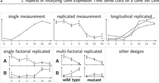
Figure 2.4 on the next page shows typical data collected for a single gene in a time
course experiment. Different experimental designs are illustrated. The simplest case
is one expression value per time point. This design of experiment does not allow
to consider the variability of the gene expression data in contrast to a replicated
time course experiment. A distinction should be made between technical replicates
(from the same individual) and biological replicates (different individuals). Only the
latter allows to consider the biological variation in the analysis, while the amount of
measurement errors can be estimated by the first one. Some approaches discriminate
between longitudinal (gene expression from the same individual observed over time)
and cross-sectional (different individuals observed at different time points) time
course experiments. The idea behind longitudinal designs is to mitigate the biological
variance. However, the measurement of gene expression destroys the cells from which
the RNA is taken. Hence, it is uncertain, whether the longitudinal design brings real
benefits for the analysis and does not falsify the results because of the intervention
in the living organism or tissue. Sometimes the (replicated) time series are divided
by a single factor as the health or the treatment status. If there is only one factor,
the proposed methods in chapter 4 can be applied. If a multi-factorial design is used
or an even more complex design (e.g. continuous cofactors), then simple gene set
activation profiles would not be the aim of the study and the proposed methods are
not applicable.
single measurement
0 2 4 8 16 24 48
replicated measurement
0 2 4 8 16 24 48
longitudinal replicated
0 2 4 8 16 24 48
single factorial replicated
0 2 4 8 16 24
B A
multi-factorial replicated
B A
wild type mutant
other designs
Figure 2.4: Most common time series types resulting from the design of experiment shown for a single gene of a gene expression microarray time series experiment. The time scale is plotted on the horizontal axis and the gene expression on the vertical axis. The measurements are shown as circles and the interpolated gene expression trajectories are drawn by straight lines. The number of time points is typically small as well as the number of replicates. Additional factors are usually discrete or categorized.
The number of genes in the experiment is normally much greater than 10,000.
The approaches proposed in this thesis allow to find differential expression profiles over time for a priori defined gene sets with respect to a reference. This reference can be a mean or median expression profile for each gene on the chip over all time points or alternatively depending on the experimental design a reference presented in Figure 2.5 can be used. Another, here not considered approach would be to use the direct previous time point as reference to focus on changes within the studied time interval.
1 . . . 3
2 T
R . . . 2
1 T
1 1
2 2 . . .
. . . T T
Figure 2.5: Three possible reference types: A reference time point within the time
series (left), a single reference measurement (center) or a reference time series with an
identical sampling scheme (right).
In microarray time series experiments there is often an additional effect besides time included, for instance the tissue, the health status or one treated and one untreated group. For the control or reference experiment there are usually less replicates available than for the time points under experimental condition. Rarely, there is data available in form of a whole control time series experiment.
Formalization and Notation
This section presents the mathematical notation used in the method chapters. Since this thesis does not focus on preprocessing the analysis is based on the preprocessed and hence logarithmized gene expression values. A single gene expression value of the m
thmeasurement for gene g at time point t is denoted by x
tjm, where
t ∈ { 1 , . . . , T }, g ∈ G ˘ = {g
1, . . . , g
G} and m ∈ { 1 , . . . , M }.
G ˘ is the whole gene universe and it is assumed, that every gene g is annotated to at least one gene set s ∈ S ˘ = {s
1, . . . , s
S} . Hence, it holds ˘ G = S
Si=1s
iand s
i⊆ G ˘ ∀s
i∈ S ˘ . The capital letters T , G , M and S describe the total numbers of time points, genes, replicates and gene sets in the analysis.
A symbol list of all used notations in the thesis is given on page 281.
Methods for the Analysis of Gene Expression Time Series
The statistical analysis of typical gene expression time course experiments is in general an explorative analysis, though the most methods provide a significance measure like a p -value or promise to hold an a priori determined significance border, for instance a family wise error rate (FWER) or a false discovery rate (FDR).
Hence, it is proven standard to evaluate findings from a microarray study in an external experiment or an independent study. The main reason for this is the small sample size, which hampers to distinguish between the effects of time, experimental condition and the omnipresent biological (and technical) variance. Another reason is the adjustment for multiple experiments (e.g. tens of thousands genes), which may result in no or only few significant findings and poor power of the method.
Therefore, the hard significance border is often mitigated to a ranked list of findings, which includes some random items.
There is an uncounted variety of published methods to analyze gene expression
time series experiments. Bar-Joseph (2004) gives an early review on analyzing this
type of data. X. Wang, M. Wu, et al. (2008) list analysis strategies with an emphasis
on clustering and incorporation of multi-source information. Gene-module level
analysis, hence the identification of gene groups and the group interactive dynamics
is the topic of a review by X. Wang, Dalkic, et al. (2008). A more recent review
by Coffey and Hinde (2011) focuses on the functional data analysis (FDA) of gene
expression microarray time courses. It is not the intention of this work to explain all
these procedures in detail, but to give a survey about the main fields in this research area, which will shed a light on the great importance of this data type.
Sima, Hua, and Jung (2009) provide a survey about the inference of gene regulatory networks (GRN) based on gene expression time course experiments. A large number of samples is needed to estimate GRNs while the total number of genes is typically restricted (e.g. G = 9 genes in Bansal, Gatta, and Di Bernardo (2006)). The inference of GRN does not make use of the strength of micoarrays to provide information about tens of thousands genes, but yields relevant insights into the microbiological gene-to-gene interactions. The outcome of a GRN analysis can be used as a gene set definition in the framework of a comprehensive gene set analysis.
A second way to analyze gene expression time series is to identify genes, which are differentially expressed across the examined time period. This single gene analysis is described in more detail in section 3.1. The influence of the noise on the single gene results is quite large and hence a gene set analysis is often applied as second stage in the analysis, but the temporal information is in general lost on this level and hard to reconstruct.
The idea that a similar gene expression trajectory over time indicates a common function or contribution to the same biological process is the foundation of the various existing clustering approaches for the analysis of gene expression time series.
Section 3.2 gives a brief overview of the methods proposed in the literature. Most clustering approaches provide an exhaustive partition of the gene universe and hence allow formulation of hypotheses for the function of genes, where this information is not yet available. Conversely, the hard cut between the clusters seems not to be a good assumption for modeling the complex interaction between the true biologic processes, because one gene product may contribute to different biological processes in different cell states.
There are methods which does not fit into the three former categories. Those,
which are related to gene set analysis are summarized in section 3.3. Some others are
designed to identify genes jointly regulated by so called transcription factors (TFs) in
time series experiments (Das, Nahlé, and M. Q. Zhang 2006; L. Wang, G. Chen, and
Li 2007). Holter, Maritan, et al. (2001) attempt to explore the causal relationship
among genes by deducing a time translational matrix on the characteristic modes specified by singular value decomposition (SVD). Gene expression time series data is also used to identify regulatory modules and condition-specific regulators (Segal, Shapira, et al. 2003). The discovery of genes with periodic gene expression may also be an analytic goal, see J. Chen and Chang (2008) for a review. Hirose, Yoshida, et al. (2008) attempt to simultaneously identify transcriptional modules (gene sets) and analyze the resulting module-based networks within a state space model, whose applicability is limited to time series with more than ten time points and a comparatively small number of genes (several thousands). Still other approaches face the task of classifying time series profiles in categories according to prototypes of trajectories over time. Such a model gene expression pattern can be acquired from previous experiments with respect to molecular reaction to toxins (Hafemeister, Costa, et al. 2011) or in relation to the progress of a disease (Costa, Schönhuth, Hafemeister, et al. 2009). Finally, there are methods to analyze gene expression time series in order to identify the different timing of gene expression under certain conditions (Yoneya and Mamitsuka 2007) or to distinct between a consensus gene expression trajectory and an individual response to a drug in clinical studies (Kaminski and Bar-Joseph 2007).
In the following the focus lies on published methods, which allow to analyze time series experiments on the level of a priori defined gene sets.
3.1 Gene Set Testing Based on Differentially Expressed Genes
In principle, all methods providing a list of significant genes can be used for an
enrichment analysis on the gene set level. By using just the list of genes significantly
changing their expression over time has the drawback of loosing all information
about the form of differential expression across the examined time points. Another
disadvantage is the large influence of noise on the resulting gene list and hence its
bad performance in terms of reproducibility.
Nevertheless, methods identifying significant differences in the gene expression values across time are largely used. They can be roughly grouped by the way they assign significance to the gene trajectories.
Three statistics to identify significantly differentially expressed genes between two equally sampled gene expression time courses are proposed by Di Camillo, Toffolo, et al. (2007). The method uses the maximal difference or the area between the linear or spline interpolated gene expression measurements across the given time points. The significance assessment follows from various null distributions estimated by using replicate measurements.
Some approaches provide a gene ranking according to differential expression across time. Chuan Tai and Speed (2009) use a multivariate empirical Bayes approach to sort genes according to their differential expression within one or between two or more gene expression time series (i.e. two or more experimental conditions besides time). Kalaitzis and Lawrence (2011) rank differentially expressed genes through a likelihood ratio quotient or a Bayes factor after modeling gene trajectories by Gaussian process regression. The approach of Cheng, X. Ma, et al. (2006) investigates the changes in an estimated gene neighborhood by the mean absolute rank difference (MARD) and hence relies completely on gene expression ranks per time point.
Other methods directly model the gene expression under various conditions and experimental designs directly on the discrete sampled time series. Xu, Olson, and Zhao (2002) use a regression based statistical modeling approach in combination with permutation tests to find significantly differentially expressed genes. Limma is a very popular procedure fitting linear models to the gene expression values and using moderated tests in the analysis of variance (ANOVA) framework to assign significance to its findings (G. K. Smyth 2004; G. Smyth 2005). Park, Yi, et al. (2003) apply ANOVA models in combination with F – or permutation tests to identify significant time-group-interactions or effects of experimental groups.
ElBakry, Ahmad, and Swamy (2012) propose a modified repeated measure ANOVA,
which removes the variance caused by individual differences and assigns significance
per permutation of columns (i.e. within time points and replicates). The idea of
M. J. Nueda, Conesa, et al. (2007) is to utilize a principal componant analysis (PCA) for a dimension reduction of the estimated parameters from an ANOVA model in multiple series time course experiments. Genes contributing to a significant effect in this so called ANOVA-SCA model are identified by permutation tests on the leverage or squared prediction error.
Hidden Markov models (HMM) are a further class of statistical tools applied in the gene-wise analysis of gene expression time-course experiments. Yuan and Kendziorski (2006) estimate non-homogeneous HMMs to distinguish between the two states equally expressed and differentially expressed at each time point. Hidden spatial-temporal Markov random fields are used by Wei and Li (2008) to identify genes, which are differentially expressed at each time point in the context of known biological pathways.
A wide range of methods originates from the field of functional data analysis (FDA).
They have in common, that the measured gene expression trajectory is modeled as continuous function in time. Bar-Joseph, Gerber, Simon, et al. (2003) apply gene-wise hypotheses testing on the integral of the quadratic difference between the B -spline curves of two aligned gene expression time series experiments. Storey, Xiao, et al.
(2005) introduce the popular Extraction of Differential Gene Expression (EDGE) software and method for the identification of differentially expressed genes. The procedure fits a natural cubic spline representation of the gene expression trajectory under the alternative hypothesis and a constant mean curve under the null hypothesis.
Permutation testing based on the residual sums of squares of both models assigns
significance to the detected differentially expressed genes. A functional hierarchical
model on the p -dimensional B -spline basis gene expression curves is utilized by Hong
and Li (2006). Bayesian Analyisis of Time Series (BATS) is a software tool proposed
for one-sample time series (Angelini, De Canditiis, et al. 2007; Angelini, Cutillo,
et al. 2008). The functional Bayesian approach expands the gene temporal profiles
over an orthonormal basis and assigns significance for differential gene expression
in the form of Bayes factors. P. Ma, Zhong, and J. Liu (2009) utilize a functional
ANOVA mixed-effects model to identify either non-parallel differentially expressed
genes or parallel differentially expressed genes. X. Liu and Yang (2009) apply a
functional principal component analysis to test for changes in the temporal gene expression under different conditions.
The advantage of gene wise approaches is the consideration of all transcripts measured on the chip. Hence, hypotheses about unknown gene-functions can be made. The power of gene-wise approaches is low, because smaller effects caused by an experimental factor will not show up on a top position in the list of significant genes and are therefore not considered for a detailed view. Although a subsequent gene set testing step based on the gene-wise tests mentioned above would be straightforward and would give additional insights into the underlying biology, it is not very often applied in the literature. The clustering approaches in the next section are more often combined with an analysis of predefined gene sets.
3.2 Clustering Approaches
Clustering approaches intend to identify groups of genes with a coherent gene expression over time. The underlying idea of these procedures is, that the similar gene expression trajectory results from a common cause (e.g. a transcription factor) or a common function. The clustering methods can be discriminated in three main fields the similarity based approaches, the model based procedures and template based methods, which attempt to recognize genes with a gene expression time profile similar to predefined patterns.
Similarity based gene clusters can for instance be found by simple visual inspection
(Cho, Campbell, et al. 1998). Some clustering algorithms need a predetermined
total number of clusters as the k -means procedure (Tavazoie, Hughes, et al. 1999)
or in the self organizing map (SOM) framework (Tamayo, Slonim, et al. 1999). The
standard agglomerative hierarchical clustering has been applied by Eisen, Spellman,
et al. (1998) or Magni, Ferrazzi, et al. (2008), the latter provide the software
package TimeClust , which implements several clustering techniques (e.g. Bayesian
clustering). Brown, Grundy, et al. (2000) propose to use a supervised learning
algorithm, which is based on support vector machines (SVMs), to group genes with
unknown function to clusters with a priori known function. The CLICK algorithm (Sharan, Shamir, et al. 2000) combines graph-theoretical and statistical techniques to find homogeneous gene expression clusters. J. Kim and J. H. Kim (2007) define the similarity on symbolic vectors representing the first and second order differences between adjacent time points. Gene Shaving is introduced by Hastie, Tibshirani, et al. (2000) as a cluster algorithm, which applies sequential PCA techniques to identify those genes, which are both largely varying across time and coherent to each other. Tchagang, Bui, et al. (2009) propose clustering in a rank order preserving matrix framework or by identifying minimum mean squared residue clusters.
The second type of cluster procedures groups the genes either based on the model fit of their gene expression trajectory in time, by the application of a specific clustering model, or a combination of both. Ben-Dor, Shamir, and Yakhini (1999) propose a corrupted clique graph model for the non-hierarchical clustering of genes.
Fitting a mixture of multivariate Gaussian distributions to the gene expression values is the approach of Yeung, Fraley, et al. (2001) available in the MCLUST software package. Šášik, Iranfar, et al. (2002) attempt to cluster genes involved in a specific biological process based on a biological kinetic model. The expectation maximization (EM) algorithm is used by Bar-Joseph, Gerber, Gifford, et al. (2002) to cluster genes on the basis of their cubic spline representation in a predefined number of sets.
Ramoni, Sebastiani, and Kohane (2002) introduce CAGED (Cluster analysis of gene
expression dynamics), a pseudo-Bayesian agglomerative clustering approach applied
on auto-regressive gene expression models. An extension of this procedure based on
polynomial models for describing the gene expression trajectory in the framework
of a Bayesian hierarchical mixture model was published by L. Wang, Ramoni, and
Sebastiani (2006). Luan and Li (2003) utilize the EM algorithm to fit a mixed
effects model on the B-spline representations of the gene expression profiles. The
EM algorithm is also used by Chudova, Hart, et al. (2003) for modeling a mixture
of simplified differential equations in order to cluster genes according to their gene
expression time course. Schliep, Schonhuth, and Steinhoff (2003) applied model
based clustering based on linear HMMs, which is implemented in the Graphical
Query Language (GQL) (Costa, Schönhuth, and Schliep 2005). An approach to
infer gene clusters from finite mixtures of HMMs while using prior informations in a semisupervised learning framework is proposed by Schliep, Costa, et al. (2005). The approach called maSigPro (microarray significant profiles) identifies gene clusters of differentially expressed genes by a two-step regression approach, where the algorithm is based on the similarity of the gene-wise regression model coefficients (Conesa, M. J.
Nueda, et al. 2006). Heard, Holmes, and Stephens (2006) introduces a Bayesian hierarchical clustering of nonlinear regression spline representation of the gene expression trajectories. A mixture of mixed-effects models, which applies a rejection controlled EM algorithm to estimate the class assignment and the corresponding mean expression curves is used by P. Ma, Zhong, and J. Liu (2009). Scharl, Grün, and Leisch (2010) find clusters using the EM algorithm to fit mixtures of linear models or linear mixed models.
Template based methods attempt to identify predefined patterns in the temporal
gene expression trajectories. In contrast to most other clustering approaches signifi-
cance can be assigned to the various template clusters by permutation or resampling
procedures. Peddada, Lobenhofer, et al. (2003) propose an order-restricted inference
methodology defining candidate temporal profiles in terms of inequalities among the
mean expression levels at the time points. T. Liu, N. Lin, et al. (2009) introduce the
ORICC algorithm, which groups the gene trajectories according to an order-restricted
information criterion to pre-specified candidate inequality profiles. A hierarchy of
trend temporal abstraction profiles (consisting of steady, increasing, decreasing)
serve as prototypes for the clustering of the gene expression profiles in the approach
of Sacchi, Bellazzi, et al. (2005). The EPIG method uses a multi-step filtering
procedure to generate representative candidate patterns from the data (Chou, Zhou,
et al. 2007). StepMiner software (Sahoo, Dill, et al. 2007) identifies genes with
one or more binary transitions across the gene expression time series by modeling
segment-wise constant adaptive regression. Ramakrishnan, Tadepalli, et al. (2010)
introduce the GOALIE procedure, which uses linear time logics to identify segments
in the time series and separate gene clusters with coherent gene expression behavior
within the segments. Ernst and Bar-Joseph (2006) implemented their method in
the Short Time-series Expression Miner (STEM) software. The STEM procedure
matches the gene expression profiles on data-independent chosen model profiles and applies a time point permutation test to assign significance to the corresponding gene clusters. A Fisher test is used to identify GO gene sets enriched with genes from significant clusters. Springer, Ickstadt, and Stoeckler (2011) propose a data-driven selection of model profiles, which gains a better fit to the data structure, but with the drawback of loosing the significance assessment for the identified clusters.
An own implementation of the STEM method based on the median gene expression profiles is used to compare the performance of the proposed methods (see chapter 4) in a simulation setting (see chapter 5) and for the example data sets (see chapter 6).
3.3 Other Approaches for the Gene Set Analysis of Gene Ex- pression Time Series
There are published methods, which do not fit in the former two main categories, but attempt to analyze gene expression time series on a gene set level. Hvidsten, Lægreid, and Komorowski (2003) propose a systematic supervised learning approach to generate hypotheses about the function of genes not yet annotated to any considered predefined GO gene set. The procedure is based on learning a classification rule model within the rough set framework, which is evaluated by cross validation. Other approaches assume that the gene expression of all genes in a predefined gene set follows the same trajectory, which is hence estimated by regarding the genes as multiple measurements of the same pattern in time. The GlobalANCOVA procedure by Hummel, Meister, and Mansmann (2008) fits a linear model to the gene expression values for every gene set and identifies those groups, in which a design factor (e.g.
treatment-time interaction) is significant in contrast to a reduced model. L. Wang,
X. Chen, et al. (2009) construct a unified mixed effects model for the mean trajectory
of every gene set and claim that their algorithm detects gene sets, in which at least
20 – 50 % of the genes follow the same linear trend. A nonparametric Wald-type
test statistic in combination with a permutation based test is used by K. Zhang,
H. Wang, et al. (2011) to detect treatment effects or treatment-time interactions
in predefined gene sets. The principal components analysis through conditional expectation (PACE) is proposed by Yao, Muller, and J. Wang (2005) to estimate the mean trajectory function for sparse longitudinal data and apply it on yeast cell cycle gene sets. The idea of fitting regression models to the gene set gene expression values in the time series or to the corresponding principal components is introduced by M. Nueda, Sebastián, et al. (2009), who denote their method as maSigFun or respectively as PCA-maSigFun . The first approach assumes, that all group genes follow the same underlying trajectory, but the second allows for more than one model profile per group, but due to the regression on the principal components, the group profile is hard to reconstruct. The maSigFun is used as competitor in the simulation study (see chapter 5 and the data analysis (see chapter 6). A brief introduction to the method is given in section 4.7. The implementation maintained in the original article is used.
None of the approaches for the analysis of gene expression time series known to
the author intends to estimate an activity profile for an a priori defined gene set. The
assumption that all or at least a majority of genes in a gene set defined by its general
function follows a common gene trajectory is very strict and counterexamples may
easily be found. Imagine complex functions like embryonic development or immune
response, whose gene expression in healthy organisms needs to be well balanced and
fine-tuned. Hence, it is implausible that all genes related to those general processes
show the same (functional) expression trajectory at all possible time points. This
thesis focuses on the idea to identify a gene set activity with respect to a reference
at the examined time points and the therefor proposed methods are the subject of
the next chapter.
Estimating Temporal Activation Profiles of Gene Sets
In contrast to the numerous approaches proposed in the literature to analyze gene expression time series the objective of this thesis is to estimate a temporal activation profile with respect to a reference for an a priori defined gene set. Most existing methods which intent to make use of the knowledge provided by reasonably defined gene sets focus on the clustering of genes with a common differential expression profile or use a significance measure on the gene wise differential expression before a common gene set enrichment test is applied (see chapter 3). Most common gene set definitions are mentioned in section 2.2. It seems to be a promising approach to estimate an activation profile over the examined time points for every gene set of interest in order to obtain an exploratory view into the molecular functions summarized by the gene set of the current definition. For instance, it allows the researcher in a way of helicopter view to obtain a sight on the bigger picture of biological functions or protein pathways without getting lost in the list of hundreds of significant genes.
Since genes interact in a way that gene products of an early stage gene may
suppress the gene expression of their own genetic information, but promote the gene
expression of other genes (e.g. those in a following stage of the pathway), an average
gene expression profile seems not to be a good representation for the activation of a
gene set. The proposed approaches in this chapter therefore are derived from ideas
from enrichment testing for the analysis of two condition gene expression microarray
experiments, which are described in section 4.1.
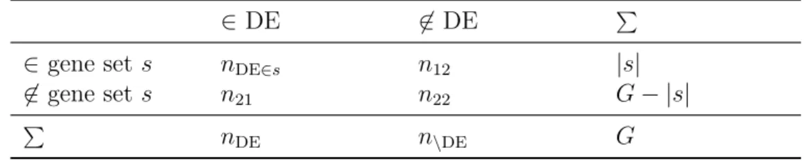
The proposed algorithms follow a three stage procedure, which is illustrated in Figure 4.1 on the next page. The input of the algorithms includes the preprocessed gene expression values for the time points and reference, the gene set definitions, and parameters for testing and smoothing. The first step provides the information of differential expression with respect to the reference for all genes and every time point either qualitative (up, down, not different), ordinal (ranked gene list) or quantitative (shrunken t -test values). The second step identifies gene sets which are enriched with up or down expressed genes. The three algorithms use different statistical tests to detect enrichment, either as over representation of differential expressed genes in the sets (Fisher test) or as asymmetric distribution of the gene set genes across the ranked list (segment test and GSEA like test). These profile algorithms are described in sections 4.2 and 4.5. Smoothing of non-reliable alternating profiles, which are hard to biologically interpret is the final step of the algorithms. The smoothing algorithms, which are evaluated by a simulation study in chapter 5, are explained in detail in section 4.3. A proposal to rank the resulting temporal activation profiles is given in section 4.4.
All methods described in chapters 4 and 5 are implemented in R -code (using
R -version 2.14.3, see R Development Core Team (2012)) programmed by the author
and is available on request.
Input
• Time series gene expression matrix
• Gene group annotation (definition of gene sets, e.g. GO)
• Parameters for multiple testing adjustment: α
genes, α
sets• Smoothing algorithm (including smoothing parameters)
Identification of differentially expressed genes
• Determine up and / or down expressed genes for every time point with respect to the reference
• shrunken t -tests to find significant differences per gene and time point
T sets of significant genes per time point
ranked gene list accord- ing to differential expres- sion per time point
G×T matrix of shrunken t -statistic values
Identification of enriched gene sets
Test every gene set at every time point for enrichment with up and / or down expressed genes and (optional) FDR-adjustment for multiple testing
Fisher test per gene set
and time point segment test per gene
set and time point GSEA like rotation test per set and time point
Smoothing of alternating activation profiles
Apply algorithms to smooth alternating profiles that are biologically not meaningful
Output
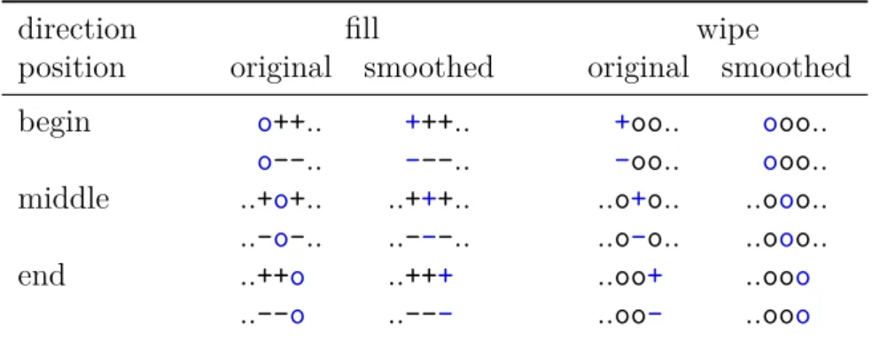
Symbolic temporal activation profile for every gene set (e.g. ’ ++oo-- ‘)
Figure 4.1: Schematic illustration of three possible algorithms for the estimation of
gene set activation profiles. The differences of the three methods are shown in the
intermediate steps enclosed by solid (threshold variant of the GSA-type algorithm),
dashed (non-threshold GSA-type algorithm), or dotted (GSEA by rotation testing)
line.
4.1 Methods Adapted from Gene Set Testing For Two Condition Gene Expression Experiments
Microarray studies conducted to compare only two conditions or respectively a single bivariate experimental factor (e.g. healthy and diseased or stem cell and differentiated cell) often provide much more replicates per condition than time series experiments. Hence, in the gene set analysis (GSA) of such experiments permutation and resampling approaches (either for the condition label or the genes) are quite common to estimate the null distribution of an enrichment test. The order of measurements is not arbitrary in time series experiments and the assumption of the exchangeability of genes seems not to be justified, since the gene expression is obviously correlated. Due to these reasons only those methods can be regarded, which can abandon permutation and resampling.
Detection of Differentially Expressed Genes
Cui and Churchill (2003) give a review of most common statistical tests for differential expression in gene expression experiments. In case of no replicates the relative gene expression of case and control samples – the so called fold change – is applied. If the expression values are assumed to be logarithmized to base two, the fold change for a gene g is defined as:
FC
g= 2
xBg−xAg,
where A and B denote the two different experimental conditions. If the assumption of equal variances across the gene expression intensities is made (which is usually not true), an average fold change can be applied.
The t -test is a standard method to detect differential expression if replicates are
available. Despite its optimality for normal distributed data it is also applicable for
other distributions. The test statistic is calculated as:
D
t−testg= x ¯
Bg− x ¯
Agsd
g,
where sd
gdenotes the sample estimate of the standard deviation, provided by
sd
g= q v
gA/M
A+ v
gB/M
Bv
gA/B= 1 M
A/B− 1
MA/B
X
m=1
x
A/Bgm− x ¯
A/Bg2
and the sampling means for gene g are given by
¯
x
A/Bg= 1 M
A/BMA/B
X
m=1