Analysis of optimal differential gene expression
D I S S E R T A T I O N
zur Erlangung des akademischen Grades doctor rerum naturalium
(Dr. rer. nat.)
im Fach Biophysik/Theoretische Biophysik eingereicht an der
Mathematisch-Naturwissenschaftlichen Fakult¨ at I Humboldt-Universit¨ at zu Berlin
von
Herr Dipl.-Phys. Wolfram Liebermeister geboren am 25.7.1972 in T¨ ubingen
Pr¨ asident der Humboldt-Universit¨ at zu Berlin:
Prof. Dr. J¨ urgen Mlynek
Dekan der Mathematisch-Naturwissenschaftlichen Fakult¨ at I:
Prof. Dr. Michael Linscheid Gutachter:
1. Prof. Dr. Reinhart Heinrich 2. Prof. Dr. Thomas H¨ ofer 3. Prof. Dr. Martin Vingron
eingereicht am: 21. Mai 2003
Tag der m¨ undlichen Pr¨ ufung: 13. Januar 2004
Abstract
This thesis is concerned with the observation that coregulation patterns in gene expression data often reflect functional structures of the cell. First, simulated gene expression data and expression data from yeast experiments are studied with independent component analysis (ICA) and with related factor models. Then, in a more theoretical approach, relations between gene expression patterns and the biological function of the genes are derived from an optimality principle.
Linear factor models such as ICA decompose gene expression matrices into statistical com- ponents. The coefficients with respect to the components can be interpreted as profiles of hidden variables (called “expression modes”) that assume different values in the different samples. In contrast to clusterings, such factor models account for a superposition of effects and for individual responses of the different genes: each gene profile consists of a superposition of the expression modes, which thereby account for the common variation of many genes. The components are estimated blindly from the data, that is, without further biological knowledge, and most of the methods considered here can reconstruct al- most sparse components. Thresholding a component reveals genes that respond strongly to the corresponding mode, in comparison to genes showing differential expression among individual samples.
In this work, different factor models are applied to simulated and experimental expres- sion data. To simulate expression data, it is assumed that gene expression depends on several unobserved variables (“biological expression modes”) which characterise the cell state and that the genes respond to them according to nonlinear functions called “gene programs”. Is there a chance to reconstruct such expression modes with a blind data analysis? The tests in this work show that the modes can be found with ICA even if the data are noisy or weakly nonlinear, or if the numbers of true and estimated components do not match. Regression models are fitted to the profiles of single genes to explain their expression by expression modes from factor models or by the expression of single tran- scription factors. Nonlinear gene programs are estimated by nonlinear ICA: such effective gene programs may be used for describing gene expression in large cell models. ICA and similar methods are applied to expression data from cell-cycle experiments: besides bi- ologically interpretable modes, experimental artefacts, probably caused by hybridisation effects and contamination of the samples, are identified. It is shown for single components that the coregulated genes share biological functions and the corresponding enzymes are concentrated in particular regions of the metabolic network.
Thus the expression machinery seems to portray - as an outcome of evolution - functional relationships between the genes: regarding the economy of resources, it would probably be inefficient if cooperating genes were not coregulated. To formalise this teleological view on gene expression, a mathematical model for the analysis of optimal differential expression (ANODE) is proposed in this work: the model describes regulators, such as genes or enzymes, and output variables, such as metabolic fluxes. The system´s be- haviour is evaluated by a fitness function, which, for instance, rates some of the metabolic fluxes in the cell and which is supposed to be optimised. This optimality principle defines an optimal response of regulators to small external perturbations. For calculating the optimal regulation patterns, the system to be controlled needs to be known only par- tially: it suffices to predefine its possible behaviour around the optimal state and the local shape of the fitness function. The method is extended to time-dependent perturba- tions: to describe the response of metabolic systems to small oscillatory perturbations, frequency-dependent control coefficients are defined and characterised by summation and connectivity theorems. For testing the predicted relation between expression and function, control coefficients are simulated for a large-scale metabolic network and their statistical properties are studied: the structure of the control coefficients matrix portrays the net- work topology, that is, chemical reactions tend to have little control on distant parts of the network. Furthermore, control coefficients within subnetworks depend only weakly on the modelling of the surrounding network.
Several plausible assumptions about appropriate expression patterns can be formally de- rived from the optimality principle: the main result is a general relation between the behaviour of regulators and their biological functions, which implies, for example, the coregulation of enzymes acting in complexes or functional modules. In this context, the functions of genes are quantified by their linear influences (called “response coefficients”) on fitness-relevant cell variables. For enzymes controlling metabolism, the theorems of metabolic control theory lead to sum rules that relate the expression patterns to the struc- ture of the metabolic network. Further predictions concern a symmetric compensation for gene deletions and a relation between gene expression and the fitness loss caused by gene deletions. If optimal regulation is realised by feedback signals between the cell variables and the regulators, then functional relations are also portrayed in the linear feedback coefficients, so genes of similar function may be expected to share inputs from the same signalling cascades. According to the model of optimal regulation, expression profiles are linear combinations of response coefficient profiles: tests with experimental expres- sion profiles and simulated control coefficients support this hypothesis, and the common components which are estimated from both kinds of data provide a vivid picture of the metabolic adaptations that are required in different environments.
To summarise, empirical relations between gene expression and function have been con- firmed in this work. Furthermore, such relations have been predicted on theoretical
grounds. A main aim is to clarify teleological assertions about gene expression by de- riving them from explicit assumptions, and thus to provide a theoretical framework for the integration of expression data and functional annotations. While other authors have compared expression to functional gene categories or topologically defined metabolic path- ways, I propose to relate it to the response coefficients. A main result of this work is that general relations are predicted between a gene’s function, its optimal expression behaviour, and its regulatory program. Where the assumption of optimality is valid, the model justi- fies the use of expression data for functional annotation and pathway reconstruction, and it provides a function-related interpretation for the linear components behind expression data. The methods from this work are not limited to gene expression data: the factor models are applicable to protein and metabolite data as well, and the optimality principle may also apply to other regulatory mechanisms, such as the allosteric control of enzymes.
Keywords:
differential expression, optimal control, metabolic control theory, gene function
Zusammenfassung
Diese Doktorarbeit behandelt die Beobachtung, daß Koregulationsmuster in Genexpressi- onsdaten h¨aufig Funktionsstrukturen der Zelle widerspiegeln. Zun¨achst werden simulierte Genexpressionsdaten und Expressionsdaten aus Hefeexperimenten mit Hilfe von Indepen- dent Component Analysis (ICA) und verwandten Faktormodellen untersucht. In einem eher theoretischen Zugang werden anschließend Beziehungen zwischen den Expressions- mustern und der biologischen Funktion der Gene aus einem Optimalit¨atsprinzip hergelei- tet.
Lineare Faktormodelle, beispielsweise ICA, zerlegen Genexpressionsmatrizen in statisti- sche Komponenten: die Koeffizienten bez¨uglich der Komponenten k¨onnen als Profile von verborgenen Variablen (“Expressionsmoden”) interpretiert werden, deren Werte zwischen den Proben variieren. Im Gegensatz zu Clustermethoden beschreiben solche Faktormo- delle eine ¨Uberlagerung biologischer Effekte und die individuellen Reaktionen der einzel- nen Gene: jedes Genprofil besteht aus einer ¨Uberlagerung der Expressionsmoden, die so die gemeinsamen Schwankungen vieler Gene erkl¨aren. Die linearen Komponenten wer- den blind, also ohne zus¨atzliches biologisches Wissen, aus den Daten gesch¨atzt, und die meisten der hier betrachteten Methoden erlauben es, nahezu schwach besetzte Kompo- nenten zu rekonstruieren. Beim Ausd¨unnen einer Komponente werden Gene sichtbar, die stark auf die entsprechende Mode reagieren, ganz in Analogie zu Genen, die differentielle Expression zwischen einzelnen Proben zeigen.
Verschiedene Faktormodelle werden in dieser Arbeit auf simulierte und experimentelle Ex- pressionsdaten angewendet. Bei der Simulation von Expressionsdaten wird angenommen, daß die Genexpression von einigen unbeobachteten Variablen (“biologischen Expressions- moden”) abh¨angt, die den Zellzustand beschreiben und deren Einfluss auf die Gene sich durch nichtlineare Funktionen, die sogenannten Genprogramme, beschreiben l¨aßt. Be- steht Hoffnung, solche Expressionsmoden durch blinde Datenanalyse wiederzufinden? Die Tests in dieser Arbeit zeigen, daß die Moden mit ICA recht zuverl¨assig gefunden wer- den, selbst wenn die Daten verrauscht oder leicht nichtlinear sind und die Anzahl der wahren und der gesch¨atzten Komponenten nicht ¨ubereinstimmt. Regressionsmodelle wer- den an Profile einzelner Gene angepasst, um ihre Expression durch Expressionsmoden aus Faktormodellen oder durch die Expression einzelner Transkriptionsfaktoren zu er- kl¨aren. Nichtlineare Genprogramme werden mit Hilfe von nichtlinearer ICA ermittelt:
solche effektiven Genprogramme k¨onnten zur Beschreibung von Genexpression in großen Zellmodellen Verwendung finden. ICA und verwandte Methoden werden auf Expressions- daten aus Zellzyklusexperimenten angewendet: neben biologisch interpretierbaren Moden
werden experimentelle Artefakte identifiziert, die vermutlich Hybridisierungseffekte oder eine Verunreinigung der Proben widerspiegeln. F¨ur einzelne Komponenten wird gezeigt, daß die koregulierten Gene gemeinsame biologische Funktionen besitzen und daß die ent- sprechenden Enzyme bevorzugt in bestimmten Bereichen des Stoffwechselnetzes zu finden sind.
Die Expressionmechanismen scheinen also - als Ergebnis der Evolution - Funktionsbe- ziehungen zwischen den Genen widerzuspiegeln: es w¨are unter ¨okonomischen Gesichts- punkten vermutlich ineffizient, wenn kooperierende Gene nicht auch koreguliert w¨urden.
Um diese teleologische Vorstellung von Genexpression zu formalisieren, wird in dieser Arbeit ein mathematisches Modell zur Analyse der optimalen differentiellen Expressi- on (ANODE) vorgeschlagen: das Modell beschreibt Regulatoren, also beispielsweise Ge- ne oder Enzyme, und die von ihnen gesteuerten Variablen, zum Beispiel metabolische Fl¨usse. Das Systemverhalten wird durch eine Fitnessfunktion bewertet, die beispielsweise von bestimmten Stoffwechselfl¨ussen abh¨angt und die es zu optimieren gilt. Dieses Op- timalit¨atsprinzip definiert eine optimale Reaktion der Regulatoren auf kleine ¨außeren St¨orungen. Zur Berechnung optimaler Regulationsmuster braucht das zu regulierende Sy- stem nur teilweise bekannt zu sein: es gen¨ugt, sein m¨ogliches Verhalten in der N¨ahe des optimalen Zustandes sowie die lokale Form der Fitnesslandschaft zu kennen. Die Methode wird auf zeitabh¨angige St¨orungen erweitert: um die Antwort von Stoffwechselsystemen auf kleine oszillatorische St¨orungen zu beschreiben, werden frequenzabh¨angige Kontroll- koeffizienten definiert und durch Summations- und Konnektivit¨atstheoreme charakteri- siert. Um die vorhergesagte Beziehung zwischen Expression und Funktion zu pr¨ufen, wer- den Kontrollkoeffizienten f¨ur ein großes Stoffwechselnetz simuliert, und ihre statistischen Eigenschaften werden untersucht: die Struktur der Kontrollkoeffizientenmatrix bildet die Netztopologie ab, das bedeutet, chemische Reaktionen haben gew¨ohnlich einen geringen Einfluss auf weit entfernte Teile des Netzes. Außerdem h¨angen die Kontrollkoeffizienten innerhalb eines Teilnetzes nur schwach von der Modellierung des umgebenden Netzes ab.
Verschiedene plausible Annahmen ¨uber sinnvolle Expressionsmuster lassen sich formal aus dem Optimalit¨atsprinzip herleiten: das Hauptergebnis ist eine allgemeine Beziehung zwi- schen dem Verhalten und der biologischen Funktion von Regulatoren, aus der sich zum Beispiel die Koregulation von Enzymen in Komplexen oder Funktionsmodulen ergibt.
Die Funktionen der Gene werden in diesem Zusammenhang durch ihre linearen Einfl¨usse (die sogenannten Responsekoeffizienten) auf fitnessrelevante Zellvariable beschrieben. F¨ur Stoffwechselenzyme werden aus den Theoremen der metabolischen Kontrolltheorie Sum- menregeln hergeleitet, die die Expressionsmuster mit der Struktur des Stoffwechselnetzes verkn¨upfen. Weitere Vorhersagen betreffen eine symmetrische Kompensation von Gende- letionen und eine Beziehung zwischen Genexpression und dem Fitnessverlust aufgrund von Deletionen. Wenn die optimale Steuerung durch eine R¨uckkopplung zwischen Zellvariablen und den Regulatoren verwirklicht ist, dann spiegeln sich funktionale Beziehungen auch in
den R¨uckkopplungskoeffizienten wider. Daher liegt es nahe, daß Gene mit ¨ahnlicher Funk- tion durch Eingangssignale aus denselben Signalwegen gesteuert werden. Das Modell der optimalen Steuerung sagt voraus, daß Expressionsprofile aus Linearkombinationen von Responsekoeffizientenprofilen bestehen: Tests mit experimentellen Expressionsdaten und simulierten Kontrollkoeffizienten st¨utzen diese Hypothese, und die gemeinsamen Kompo- nenten, die aus diesen beiden Arten von Daten gesch¨atzt werden, liefern ein anschauliches Bild der Stochwechselvorg¨ange, die zur Anpassung an unterschiedliche Umgebungen not- wendig sind.
Alles in allem werden in dieser Arbeit empirische Beziehungen zwischen der Expressi- on and der Funktion von Genen best¨atigt. Dar¨uber hinaus werden solche Beziehungen aus theorischen Gr¨unden vorhergesagt. Ein Hauptziel ist es, teleologische Aussagen ¨uber Genexpression auf explizite Annahmen zur¨uckzuf¨uhren und dadurch klarer zu formulie- ren, und so einen theoretischen Rahmen f¨ur die Integration von Expressionsdaten und Funktionsannotationen zu liefern. W¨ahrend andere Autoren die Expression mit Funkti- onskategorien der Gene oder topologisch definierten Stoffwechselwegen verglichen haben, schlage ich vor, die Funktionen von Genen durch ihre Responsekoeffizienten auszudr¨ucken.
Als ein Hauptergebnis dieser Arbeit werden allgemeine Beziehungen zwischen der Funk- tion, der optimalen Expression und dem Programm eines Gens vorhergesagt. Soweit die Optimalit¨atsannahme gilt, rechtfertigt das Modell die Verwendung von Expressionsdaten zur Funktionsannotation und zur Rekonstruktion von Stoffwechselwegen und liefert außer- dem eine funktionsbezogene Interpretation f¨ur die linearen Komponenten in Expressions- daten. Die Methoden aus dieser Arbeit sind nicht auf Genexpressionsdaten beschr¨ankt: die Faktormodelle lassen sich auch auf Protein- und Metabolitdaten anwenden, und das Opti- malit¨atsprinzip k¨onnte ebenfalls auf andere Steuerungsmechanismen angewendet werden, beispielsweise auf die allosterische Steuerung von Enzymen.
Schlagw¨orter:
Differentielle Expression, Optimale Steuerung, Metabolische Kontrolltheorie, Genfunktion
Danksagung
Ich m¨ochte zuallererst meinen Betreuern Reinhart Heinrich, Edda Klipp und Hans Lehrach danken, nicht nur f¨ur ihre Unterst¨utzung bei dieser Arbeit, sondern auch f¨ur das sch¨one und interessante Umfeld, in dem ich die letzten Jahre ¨uber lernen und arbeiten konnte.
Die Zeit in den Arbeitsgruppen an der Humboldt-Universit¨at und im Max-Planck-Institut f¨ur molekulare Genetik war f¨ur mich eine wirkliche Bereicherung, und der Abschied von meinen Mitarbeitern f¨allt mir ausgesprochen schwer. Auch zahlreiche ausw¨artige Leu- te haben mir durch Gespr¨ache bei meinem Einstieg in die Welt der Biologie geholfen und mir immer wieder neue Anregungen gegeben. Besonders erw¨ahnen m¨ochte ich hier Frank Bruggeman, Hanspeter Herzel, Femke Mensonides, Ralf Mrowka, Axel Nagel, Stef- fen Schulze-Kremer, Stefan Schuster und Rainer Spang. Ein besonderer Dank gilt auch den Kollegen, deren Daten und Algorithmen ich f¨ur meine Arbeit verwenden konnte, insbesondere A. Hyv¨arinen.
Contents
1 Introduction 1
1.1 About this work . . . 1
1.1.1 Motivation. . . 1
1.1.2 Structure of the text . . . 4
1.2 Gene expression . . . 5
1.2.1 Mechanisms of gene expression . . . 5
1.2.2 Methods for studying gene expression data . . . 7
1.3 Statistical factor models . . . 9
1.3.1 Model fitting and validation . . . 10
1.3.2 Principal components and independent components . . . 12
1.3.3 Other linear and nonlinear models. . . 15
1.4 Mathematical cell models . . . 16
1.4.1 Dynamical systems and genetic networks . . . 16
1.4.2 Metabolic control analysis . . . 17
1.4.3 Mathematical notions of information . . . 20
I Analysis of expression data 22
2 Gene programs and expression modes 23 2.1 A mathematical description of gene expression . . . 232.1.1 Gene programs and expression modes . . . 23
2.1.2 Simulated gene expression data . . . 25
2.1.3 Reducing the saturation effects in expression data . . . 27
2.2 Estimation of gene programs . . . 28
2.2.1 Estimated gene programs and expression modes . . . 28
2.2.2 Biological interpretations of expression modes . . . 29
2.2.3 Reconstructing a gene program behind artificial data . . . 31
2.2.4 Explanatory variables for gene expression. . . 31
3 Estimating gene programs by nonlinear ICA 35
3.1 Test with simulated expression data . . . 35
3.2 Application to experimental data . . . 35
3.3 Biological interpretation of nonlinear ICA . . . 40
4 Analysis of global gene expression 42 4.1 Linear components behind global expression . . . 42
4.2 Reconstructing the modes behind simulated data . . . 45
4.3 Analysis of cell cycle experiments . . . 49
4.3.1 Independent components behind cell cycle data . . . 49
4.3.2 Dimension-reduction and bootstrapping . . . 52
4.3.3 Comparing different factor models . . . 53
4.3.4 Expression modes and gene functions . . . 57
4.4 B-cell lymphoma data . . . 60
4.5 Conclusions . . . 62
II Optimal differential expression 66
5 Analysis of optimal differential expression 67 5.1 Optimal regulation of stationary states . . . 675.1.1 The mathematical model . . . 70
5.1.2 Adaptation to a perturbation of the output variables . . . 71
5.1.3 Obtaining a change of the output variables . . . 74
5.1.4 Adaptation to a perturbation of individual regulators . . . 75
5.2 Feedback signals and the value of regulators . . . 75
5.2.1 A cascade of responses . . . 75
5.2.2 Optimal control realised by feedback . . . 77
5.2.3 The value of regulators . . . 78
5.3 Predictions for gene expression patterns. . . 79
5.3.1 Correlation between functionally related genes . . . 79
5.3.2 Correlated expression of interacting proteins . . . 79
5.3.3 Symmetric compensation for deletions . . . 81
5.3.4 Growth of deletion mutants . . . 83
5.4 Examples . . . 83
5.5 Discussion . . . 88
6 Properties of optimal expression patterns 90 6.1 Perturbation of the fitness . . . 90
6.2 Constrained regulation . . . 91
6.3 Geometrical interpretation by projections . . . 93
6.4 Invariance against reassignment of regulators . . . 94
7 Time-dependent expression 96 7.1 Time-dependent gene expression . . . 96
7.2 Frequency-dependent control coefficients . . . 98
7.3 Optimal time-dependent regulation . . . 101
8 Calculation of control coefficients 103 8.1 Metabolic control coefficients. . . 103
8.1.1 Choice of the elasticities . . . 105
8.2 Distributions and correlations of control coefficients . . . 106
8.3 Resonances in metabolic control . . . 112
9 Optimal expression and function 114 9.1 Metabolic systems . . . 114
9.1.1 Sum rules derived from metabolic theorems . . . 114
9.1.2 Sum rule for the control of elementary flux modes . . . 116
9.1.3 Optimal response to flux perturbations . . . 117
9.2 Functional modules . . . 118
9.2.1 Cooperation between modules . . . 118
9.3 Relating expression to control coefficients . . . 119
9.3.1 Explaining expression data by control coefficients . . . 121
9.3.2 Similarity between gene expression and control coefficients . . . 121
9.3.3 Common components behind gene expression and control . . . 124
9.4 Discussion . . . 128
10 Conclusions 132 A Proofs and additional formulae 135 A.1 Mathematical symbols . . . 135
A.2 Derivation of Equation (5.23) . . . 136
A.3 Derivation of Equation (5.24) . . . 137
A.4 Derivation of Equation (5.26) . . . 137
A.5 Derivation of Equation (5.27) . . . 138
A.6 Derivation of Equation (5.33) . . . 138
A.7 Derivation of Equation (5.30) . . . 139
A.8 Derivation of the projector property (6.7) . . . 139
A.9 Effective fitness for constrained regulation . . . 139
B Expression data and analysis methods 141
B.1 Parameters for artificial expression data . . . 141
B.2 Data used in this work . . . 142
B.3 Algorithms. . . 142
B.4 Mapping yeast ORF to the metabolic network . . . 144
C Additional tables and figures 145
Bibliography 150
Chapter 1 Introduction
1.1 About this work
1.1.1 Motivation
Together with the physical structure of cells, their functional structure has been shaped by evolution, and the same can be assumed for regulatory processes which are responsible for coordinating the cell’s various actions [66]. This thesis is mainly concerned with the control of gene expression, which is involved in many cell processes and responses to external stimuli (see Figure 1.1). It is studied how and why expression profiles tend to portray functional structures of the cell. Genome-wide expression can be monitored by measurements with microarrays, to study which genes respond to certain experimental interventions, which of the genes show characteristic differences between cell types, and which groups of genes show a concerted effort in their expression behaviour. On the one hand, this knowledge may help to find out details about the physical mechanisms of gene expression: which transcription factors, which other signals influence a gene, and how does it respond to them? On the other hand, the cell’s expression machinery can be used as a measuring device to study the functional structure of the cell, as genes showing similar expression patterns also have a tendency to share biological functions [111] [7].
The objective of this thesis is to study these functional aspects of gene expression in more detail. I shall follow two tracks: first, coregulation structures are extracted from gene expression data by factor models. Secondly, it is assumed that the cell aims to maximise a biological fitness function and that the differential expression patterns are shaped to achieve this goal. It turns out that the resulting optimal expression patterns reflect the functions of genes, as it has been found in reality.
In many publications on gene expression, the data are organised by clusterings [26] [5], where genes and experiments with similar expression profiles are arranged into groups.
metabolism cell behaviour
cell state
signals environment
rna
expression proteins
Figure 1.1: Gene expression as a part of the cell’s regulatory network. Gene expression involves the production of messenger RNA, which is translated into proteins. Via the proteins, genes control the structure and the behaviour of the cell. Stimuli from the environment and processes within the cell send signals to the gene expression machinery.
The resulting feedback loops can ensure homoeostasis, but may also respond specifically to external stimuli, for instance, to stress conditions.
Biclustering [110] allows for a partial coregulation, detecting genes with similar profiles in subgroups of the samples. In contrast, I shall analyse expression data by linear factor models such as independent component analysis (ICA, [84] [49] [78]). Linear factor models represent the correlation structure of multivariate data by decomposing them into linear components with predefined statistical properties. A similar decomposition is used in physics, for instance, when the dynamics of a string is described by the simple behaviour of harmonics, and in metabolic control theory, where metabolic flux distributions can be superposed from elementary modes describing metabolic pathways. Compared to clus- terings, linear factor models have the advantage that each gene’s expression is explained by an individual superposition of different effects, similar to the process of transcription, where a gene may be controlled by more than just one transcription factor. The cor- responding linear transformation provides a set of general basic profiles from which the gene profiles can be superposed. In contrast to clusterings, where the expression profiles of genes are compared as a whole, genes will be regarded as coregulated here if they both respond strongly to the same expression mode, even if, due to other expression modes, the gene profile differ from each other.
Biologically, the individual yet concerted expression of genes can be attributed to an inter- play of regulatory mechanisms: in a schematical picture, the cell state can be represented by variables called “expression modes”, and each gene is controlled by a combinatorial
function (which I shall call the “gene program”), describing how the gene’s expression depends on these modes. Bussemaker et al. [9] explained expression data by a linear model where each factor influences genes that share a particular sequence motif in their regulatory regions. However, the abovementioned modes need not represent biological regulators, such as transcription factors, but may also describe the cell state in a global manner. In its mathematical form, this schematic model of expression resembles the linear models for data analysis mentioned above. The statistical factor models considered in this work estimate their components blindly from the structures in the expression data, that is, no additional biological information is used. The linear model should determine a data subspace containing the systematic effects, that is, biological processes and possibly ex- perimental artefacts, while the remaining subspace is supposed to describe weak statistical noise. A standard method for this dimension reduction is principal component analysis [22]. Furthermore, the relevant subspace should be decomposed into the separate causes of variation. This task is much more subtle: whether a method can separate distinct biological effects depends on the statistical assumptions made about the components. In this work, linear methods based on different statistical assumptions will be tested, most of which are sensitive to sparse components. As data sets, I chose publicly available data from yeast experiments, where expression during the cell cycle [107], after environmental changes [18] [10] [32], and after gene deletions [51] [61] had been studied (see Table B.3 in the appendix). For testing purposes, also simulated expression data are analysed.
As mentioned above, this work focuses on the functional aspects of gene expression: gene function can be defined qualitatively by assigning genes to functional classes, for instance to MIPS functional categories [82], gene ontology annotations [14], or KEGG metabolic pathways [64]. Such annotations state in which cellular processes or subsystems a gene is involved. Evidence for shared function can also come from associations between the gene products, for instance, for proteins forming complexes [33], interaction [112] or fusion pairs [115], or protein pairs defined by phylogenetic correlation [91] or anticorrelation.
One reason to cluster gene expression data is to determine functionally related genes: in fact, expression clusters are enriched in genes from particular functional classes [111], and genes in metabolic pathways were found to be coregulated [18]. Accordingly, expression data have been used to discriminate genes with respect to functional annotations [7] [110], to predict functions [80], or to reconstruct probable metabolic pathways [118] [38] [71].
I already stated that linear models can identify components behind gene expression data which describe concerted actions of many genes. This correlated expression might be attributed to common regulation, but the components also seem to represent common biological gene functions. A particular gene expression pattern, for instance, may be attributed to acausa efficiens, such as a signalling pathway, which physically influences the transcript levels. Accordingly, expression data have been used to identify regulatory motifs [6] [9]. On the other hand, expression may be explained by acausa finalis, namely the fact
that the gene products are needed by the cell under the given conditions. Biologists often tacitly presume a form of teleonaturalism (see [3]) where “needed by the cell” translates to “increasing the cell’s biological fitness, and thus selected for during evolution”. In biology, optimality assumption are usually justified by evolutionary arguments: caused by mutation and selection, species change their properties and thereby increase their biological fitness, that is, the long-term reproduction rate. Under a strong selection pressure a trait is likely to achieve a local optimum. This view is the basis for modelling studies on evolutionary optimisation (see, for instance, [41] [101]). Optimality of flux distributions [24] [105] has been studied, and theoretical predictions based on optimisation could be validated by experiment [60].
The optimality-based view can be extended to regulatory systems: physically, most parts of the cell can only react to processes in their immediate neighbourhood, but their func- tion would require a reaction to a distant process or condition. This discrepancy creates an evolutionary pressure on the development of signal-processing systems which distribute valuable information within the cell. If the cell is viewed as a machine, the signalling sys- tems can be seen as a hard-coded implementation of a program to control it. Accordingly, the input signals of a gene should provide primarily the information about the cell state that is relevant for the gene’s expression. A relation between the optimal regulation of enzymes and their control on fluxes has been derived in [67]. Optimal control of time- dependent processes [93] has been studied intensely and also been applied to the control of metabolic systems [68]. In this thesis, I shall formalise assertions about “sensible” gene expression by translating them into a mathematical framework.
It is assumed that gene regulation has to contribute to the optimisation of a given objective function. To define an optimal behaviour of genes, I shall consider how parts of the cell, such as metabolic subsystems, are supposed to behave, and how the genes contribute to this behaviour. In the framework of metabolic control theory [41] [42], the effects of gene expression on steady states of the metabolic system are described by the linear response coefficients, which can be calculated from the stoichiometry and the linearised kinetics of the chemical reactions. In this work, they are the key quantities to describe the function of genes, and it turns out that they also appear in the formulae for optimal expression patterns.
1.1.2 Structure of the text
The rest of this first chapter summarises concepts and methods from theoretical biology and statistical data analysis that are relevant for this thesis, namely the biological regu- lation and statistical analysis of gene expression, linear factor models, and mathematical models in cell biology. The first main topic of this thesis, the analysis of coregulation in
expression data, is treated in the chapters 2, 3, and 4. Assuming that gene expression depends on common unobserved variables, I shall study whether such variables can be es- timated from microarray data. With nonlinear ICA, time courses of the expression modes are described by the components, and gene programs are reconstructed from simulated and experimental data. In chapter 4, the components are supposed to describe linear weights of the gene programs. Independent component analysis and other linear models are applied to whole-genome data to detect biologically interpretable modes and to sep- arate them from experimental noise and artefacts. In the second main part of this work, properties of gene expression patterns are predicted from the assumption of optimal regu- lation. In chapter5, a mathematical model is proposed for predicting optimal differential expression patterns. The following chapters 6 and chapter 7add generalisations and de- tails, for instance optimal response to oscillatory perturbations. The remaining chapters are concerned with relations between optimal expression patterns and the structure of metabolic networks. Control coefficients for a large metabolic network are calculated in chapter 8. Structural knowledge, for instance, about the metabolic network, can be used to predict properties of expression patterns. To test the predictions made, expression data are compared to simulated metabolic control coefficients in chapter 9. Chapter 10 summarises the results of this thesis. The appendices contain additional information: the data sets and algorithms used are listed in the AppendixB. The mathematical proofs and a list of mathematical symbols are given in AppendixA. Appendix Ccontains additional figures and further analyses of expression data.
Parts of section 4.3 and 4.4 have already been published [78] and parts of the chapters 5 and 9 are contained in [79], which has been submitted for publication. This work was supported by the Deutsche Forschungsgemeinschaft and the German Federal Ministry of Education and Research.
1.2 Gene expression
1.2.1 Mechanisms of gene expression
This section summarises basic mechanisms of gene expression in eukaryotes. A detailed description is given in [1]. The synthesis of proteins requires the production and processing of messenger RNA (mRNA), involving the following steps: an enzyme complex, the so- called called RNA polymerase, transcribes the nucleotide sequence coding for a protein to single-stranded mRNA molecules with the complementary sequence. These transcripts are spliced in the nucleus, that is, the large intron sequences are removed, and ribosomes in the cytosol translate the mRNA to proteins. After some time (usually in the order of minutes [46]), the transcripts are degraded. The correlation between RNA and protein
levels, even per gene, is not very strong [37] [61]: this may be caused by the time-delay in translation, but also by active control of RNA processing and protein decay.
Probably all steps of expression are actively controlled, in particular the initiation of tran- scription: in eukaryotes, a complex of general transcription factors forms at the TATA box, about 25 kilo-base-pairs (kbp) ahead of the start site, and enables the polymerase to start transcription. This process is controlled by regulatory proteins which can bind specifically to sequence motifs in the regulatory region around the start site. This region can be 50 kbp in size, much larger then a typical gene. Bound regulatory proteins can control the formation of the transcription complex even from a large distance. The reg- ulatory proteins themselves are controlled by different mechanisms, including their own synthesis, ligand binding, phosphorylation, complex formation, unmasking, and control of their nuclear entry. Transcription also depends on the chromatin structure and on the methylation of cytosine in GC pairs, which both can be altered by regulatory proteins.
In prokaryotes, a gene is usually controlled by few regulators which either activate or repress the gene, while in eukaryotes, genes are controlled by many regulators acting in a complicated combinatorial manner.
The rate of mRNA synthesis reflects the biological processes that control the initiation of transcription: the initiation rate, regarded as a mathematical function of these biochem- ical signals, can be supposed to have the following properties:
• Nonlinearity: The time-averaged initiation rate can be approximated by a smooth nonlinear function of the transcription factor concentration. If binding of a tran- scriptional activator is required to enable transcription, then the probability for the binding site to be occupied is a sigmoidal function of the activator’s log concentra- tion, and the gene’s program is also sigmoidal.
• Combinatorial function: If several of the abovementioned factors are required, only certain combinations of them will trigger transcription. The resulting combi- natorial function may be described by an (artificial) neural networks [22]: neural networks are schemes to build nonlinear functions by combining simple functions ac- cording to a graph structure. They are used in regression or discrimination problems in which high-dimensional nonlinear functions must be approximated by functions that are easy to parametrise. Neural networks can be fitted to data in a sequential manner (often called ”learning”), in close analogy to physiological or evolutionary adaptation of signal-processing systems.
• Modularity: Combinatorial functions can be realised by modules in the regulatory DNA sequence. For instance (see [1]), the Drosophila morphogene ”eve”, which is active in 7 distinct stripes in the embryo, is regulated by seven modules: each of
them becomes activated by signals that are characteristic for a particular region in the developing embryo. Thus the pattern to be achieved is disposed by the structure of the regulatory function.
• Time hierarchy: Different input signals may act on different time scales. In con- trast to the momentary adaptation by transcription factors, methylation of GC pairs can ensure that a gene is permanently deactivated. Hierarchical control mechanisms may manifest themselves in a hierarchy of cell states, with different cell types on top and the momentary behaviour on bottom.
Thus expression can be described by the following schematic picture: the regulatory proteins represent the state of the cell, while the corresponding binding sites on the DNA determine how genes behave in the different states. To contribute to the cell’s fitness, each gene is supposed to show a particular expression behaviour under certain cell conditions, and probably, the combinatorial regulatory functions of genes (which will be called “gene programs” in this text) have evolved along with the required behaviour of the protein. Replication and modification of small sequence motifs (comparable to genetic programming [70]) provide an efficient way to create and adapt complex regulatory functions during evolution.
1.2.2 Methods for studying gene expression data
With many genes, the expression level differs among cell types, developmental stages, and external conditions, and this differential expression can be measured in parallel and on a genomic scale by the use of macro- or microarrays: the mRNA is extracted from a cell or tissue sample and transcribed to complementary DNA (cDNA), labelled by a fluorescent dye or by a radioactive isotope. This target cDNA is then hybridised to spots of probe cDNA or oligonucleotides on nylon filters or glass slides. The bound cDNA is quantified by scanning the fluorescence, yielding an intensity value for each spot, that is, for each gene represented in the array. The observed intensity is supposed to represent the mRNA concentration in the original sample, but the data may also be superposed by statistical noise and by artefacts originating from the sample preparation and the hybridisation procedure. A typical microarray contains several thousand spots, so all known yeast genes can be represented on one chip. Microarray data allow for studying details of the the regulatory system, but they also provide important diagnostic information, for instance for the discrimination of cancer types. Microarrays are not only used for measuring expression, but also for sequencing, to identify binding of transcription factors [76], single nucleotide polymorphisms, and to quantify genetically labelled yeast strains [35].
x2
x1 x
x
1 2
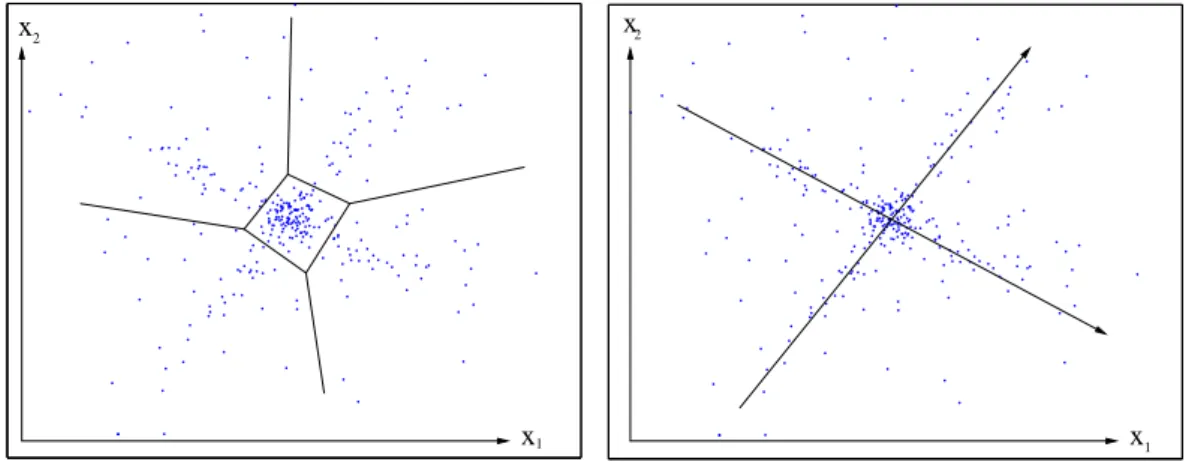
Figure 1.2: Clustering and linear factor model for multivariate data. The gene profiles are represented by points in ann-dimensional space. Its dimensions represent the expression in the different experimental samples (microarrays). In the diagrams, hypothetical data are projected to coordinates x1 and x2, which are linear combinations of the original samples. The data cloud consists of a central region of high density, surrounded by several “arms”. Clustering and factor models describe the data cloud by structures that are adapted to the cloud’s shape. Left: Clustering. The genes are grouped into different classes, according to the similarities between their profiles. Right: Linear factor model.
The data space is parametrised by new coordinates. The new basis vectors have been chosen according to the shape of the data cloud.
Microarray data form a matrix, containing the gene profiles in its rows, while the experi- mental samples (microarrays) are represented by columns. The number of genes (typically several thousand) exceeds the number of samples (usually less than a hundred). Usually, the measured intensities vary over several orders of magnitude, and both additive and multiplicative measurement errors are present: the noise level is often as high as the typ- ical differential expression among samples [23]. Systematic errors can be reduced by an accurate data normalisation [102], while statistical errors can be treated either by aver- aging over them or by estimating them as part of a statistical model. Due to the high costs, the measurements are often not repeated and usually, the noise level remains high.
This may cause severe problems because genes of interest (e.g oncogenes) may show small differential expression and remain hidden in the noise.
It is common to represent expression values by their logarithms because the error dis- tributions then become closer to normal. As the hybridisation process is not yet fully understood, it is difficult to measure absolute RNA concentrations by microarrays, and it is common to report differential expression [13] between samples or groups of samples.
An important application is to determine marker genes whose expression differs between different tumour types. For each gene, a p-value denotes the probability that the degree
of differential expression observed would occur by chance. For calculating the p-value, the biological or experimental fluctuations have to be studied by comparing repeated measurements of identical samples.
Besides differential expression and coregulation of particular genes, global patterns can be studied in expression data. In Figure1.2, hypothetical gene expression profiles, repre- sented by points, form a data cloud which has been projected to two dimensions x1 and x2. If the gene profiles are centred, then for each gene, the variance over the experiments is given by the squared distance from the cloud centre, and the correlation between two genes equals the cosine of the angle between them. Multivariate data of high dimensional- ity require methods to extract and display information about their correlation structure.
Clustering of genes determines distinct groups of genes with similar expression profiles.
K-means clustering [22], for instance, is based on the assumption that the probability density behind the data is a mixture of isotropic Gaussian distributions, each giving rise to a cluster of data points. A numberk of clusters is chosen, and the cluster centres and their members are estimated in parallel by maximum likelihood: practically, the average Euclidean distance between each data point and its respective cluster centre is minimised.
If other distance measures than the Euclidean distance are given, each cluster can be rep- resented by a data point (a so-called prototype vector), which is, on average, closest to the other points of its cluster. Hierarchical clustering [26] is a popular method to arrange genes and samples according into cluster trees. Linear factor models, which are explained in more detail in the following section, assume that the gene expression profiles can be explained by relatively few global variables. The data space is parametrised by new coor- dinates (see Figure 1.2, right), and the data can be projected to fewer dimensions. With both clustering and linear models, the results depend strongly on the data metric, which defines the similarity measure between gene profiles. The metric, in turn, depends on the normalisation scheme and on the choice and statistical weights of the experimental samples. Any preprocessing of the data effectively changes the metric, and a projection to the first principal components may yield a metric in which noise effects have less weight and the biological effects become more pronounced.
1.3 Statistical factor models
This section contains a brief overview about statistical factor models. Let us consider a pair of random variables (s, x) fulfilling
x=f(s, p) +η (1.1)
where η denotes independent Gaussian noise representing, for instance, measurement errors. The symbols x, s, and η denote vectors. If samples of both s and the x are
given, the parameterspcan be estimated by regression. In contrast to that, unsupervised methods try to infer the explanatory variables from the data: stated differently, the data variables xl are represented, according to
x=f(s) +η (1.2)
by transformed variables sk called “components” or “sources”. By this transformation, the data may be represented by fewer variables, without loss of important information:
such a dimension reduction is useful for visualising, storing, or transmitting the data, or for simplifying a further treatment, e.g., clustering or discrimination. Contrariwise, a simple sparse coding can be achieved by increasing the number of dimensions [21].
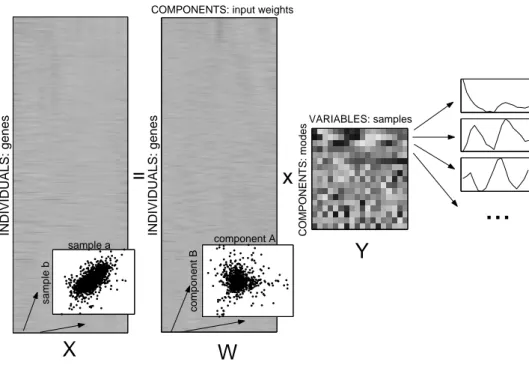
Linear models assume f to be linear, parametrised by coefficients (“loadings”) Akl. A data matrix X with rows and columns representing samples and variables1, respectively, is decomposed into
Xil = ¯µi+X
k
SikAkl+ηil (1.3)
or, in matrix notation,
X =µ+SA+η (1.4)
A is called the mixture matrix or loadings matrix. If the the data have been centred by subtracting the empirical mean µ, the linear model simply reads
X =SA+η (1.5)
1.3.1 Model fitting and validation
If constraints are imposed onS orA or if the number of variables exceeds the number of components, a decompositionX =S A+ηcan be estimated by maximising the likelihood p(X|S, A), that is, the probability to observe the data, given S and A. If the noise is independent Gaussian with zero mean and standard deviationsσik, then the log-likelihood reads
logp(X|S, A) = logpη(X−S A) =−1 2
X
ik
(X−S A)2ik
σ2ik + const. (1.6) If all σik are identical, the likelihood is maximised by minimising the sum of squared errors. In Bayesian statistics (see [34]), the model parameters (elements of S and A) are
1In the neural processing community, the convention is different, with variables in the rows and individuals in the columns.
treated as random variables drawn from a predefined prior distribution p(S, A). The log posterior probability
logp(S, A|X) = logp(X|S, A) + logp(S, A) + const. (1.7) describes the probability of certain choices of S and A after observing the data. If the prior distribution is not known, it can be parametrised by so-called hyperparameters, which are then are also treated in the Bayesian framework.
The matrix product S Ain equation 1.6 is invariant to a transformation S → S T
A → T−1 A (1.8)
and thus the result of the above maximum likelihood estimation is not unique. Also with independent component analysis (see below), the fitting criterion does not depend on the order and the signs of the components sk. Uniqueness of the solution can be forced by standardisingS andA: components can be sorted, for instance, by the data variance they explain.
If a model parameter is estimated, also the estimation error should be studied. Analyti- cally, the variance of an estimator can only be calculated for relatively simple cases. The bootstrap [25] is a method to estimate the variance of estimated parameter for unknown, empirical distributions. In principle, the variation of the estimated parameters could be studied by fitting the model for many data sets sampled from the same distribution. The bootstrap does the same thing, using virtual datasets that have been created by resam- pling from the given data. For bootstrapping linear models, the solutions from different resampling runs must be comparable: therefore a reference model is defined, and each solution is rearranged to resemble this reference model as closely as possible.
The aim in discrimination and model fitting is not to explain the data as accurately as possible, but to fit a model to the unknown underlying distribution. The model should generalise well, that is, fit new data points from the same distribution, and thus allow for prediction. Over-fitting of the given data can be detected by cross-validation: the set of samples is split into two parts, the training set and the test set. The model parameters are fitted using the training set, and a prediction error is calculated from the model predictions for the test set. This procedure is repeated for different choices of the training and the test set to calculate an average prediction error. Cross-validation can be used to determine optimal model properties, such as the best number of hidden nodes in a neural network.
1.3.2 Principal components and independent components
We saw that the matrix decomposition (1.5) is not unique. If one of the matrices is given, as with the Fourier or wavelet transform, the other one can be found by maximum likelihood estimation. Alternatively, both matrices can be identified “blindly”, that is, the new basis vectors (rows of A) are determined from the data. This requires, however, that certain statistical properties of the matrices have been specified in advance, or that a generative model with predefined statistical properties is fitted to the data. The rest of this section 1.3 gives an overview over different blind methods that have been applied to expression data or that are relevant for this work.
Principal component analysis(PCA) aims to determine components explaining maxi- mal data variance. PCA can be seen as the parameter estimation of a multivariate normal distribution, with a density
p(x)∝e−12(x−µ)T C−1 (x−µ) (1.9)
where µ and C denote the mean and the covariance matrix, respectively. PCA centres and rotates the data, using the eigenvectors of C (estimated by the empirical covariance matrix) as the new basis vectors. The respective eigenvalues describe the variances along the principal components. Except for the centring, PCA is technically equivalent to a singular value decomposition (SVD). Both the components and the new basis vectors are orthogonal on each other, that is, linearly uncorrelated. Principal components are optimal for representing maximal data variance by few components, but the separate principal components need not have an interpretation.
Independent component analysis (ICA) [54] [57] assumes statistically independent components behind the data, with a distribution
p(s) = Πi pi(si) (1.10) Practically, the ICA model
Xil =X
k
SikAkl
splits the centred data matrix into a matrix product X = SA (compare Figure 4.1 in chapter 2), subject to the condition that the statistical dependence between the columns of S be minimised. The dependence between random variables can be quantified by the mutual informationI =P
kHk−H, whereHkandHdenote the entropy of thekthvariable and the total entropy, respectively (see section 1.4.3). As the total entropy H remains constant under linear transformations, the mutual information I can be minimised by minimising the marginal entropies Hk. Among the distributions with unit variance, the normal distribution yields the maximal entropy valueHN. ICA determines directions in
the data cloud where the distribution of the data is as non-normal, and thus as informative, as possible. As a side-effect, ICA can identify components that are approximately sparse, showing many values around zero.
In this work, the FastICA algorithm by A. Hyv¨arinen [53] was used. As illustrated in Fig- ure1.3, the matrixAis split into the product A=R C1/2, where the dewhitening matrix C1/2 representing the linear correlations is calculated from the data covariance matrix C. The remaining rotation R is chosen such that the statistical dependence between the independent components is minimised. In order to avoid the time-consuming calculation of the Hk, FastICA substitutes the difference HN −Hk by a so-called contrast function
JG(k) =|hG(Sik)ii− hG(ν)i|
JG applies some even, non-quadratic function G(·) (in this work, the Gaussian function has been chosen) to each variable S·k and to a normally distributed variable ν, returning the absolute difference of the mean values. In the algorithm, the matrix R is initialised with random values and then iteratively adjusted to maximise theJG until a convergence criterion is met.
Like principal component analysis, ICA removes all linear correlations. To introduce a non-orthogonal basis, it also takes into account higher-order dependencies in the data. If the data lack such higher order structure, for instance, if they are normally distributed, the solution is not unique. The ICA model leaves some freedom to scale and sort the com- ponents: by convention, the independent components are scaled to unit variance, while their signs and their order can be chosen arbitrarily. The number of independent com- ponents equals the number of variables, but it may be reduced, for instance by removing weak principal components before applying the ICA, which considerably decreases the computational costs.
If the data fulfil the independence assumption (1.10), sparse components are easily found by ICA. Real data are probably noisy and the components are not exactly independent.
There exist many variants of ICA with different assumptions about the distribution of the components. Noisy ICA explicitly takes into account additive noise. A supergaussian distribution for the mixing matrix can be easily implemented by modifying the data used in the FastICA algorithm [58]. Components estimated by ICA will still not be exactly independent. The remaining dependencies cannot be removed by a linear transformation, but they can be distributed differently between the components: independent subspace analysis [55] and topographic ICA [56] explicitly assume the existence of higher-order de- pendencies between the components, and try to distribute them among the components in a controlled way. Independent subspace analysis aims at concentrating the mutual information within subspaces of fixed dimensionality. With topographic ICA, a (usu- ally grid-like) topology between the components is prescribed, and the components are
−5 0 5
−5 0 5
−5 0 5
−5 0 5 −5 0 5
A
B
C
D
E
F
Figure 1.3: Independent component analysis of artificial data. Left: A cloud of n data points was produced by (A) choosing independent coordinates S1 and S2 from the two- sided exponential distribution and (B) shearing the data cloud by a linear transformation A. The centred data are contained in a n×2 matrixX. ICA reconstructs the unsheared data up to scaling, permutation, and reflection of the axes, based on the knowledge that the coordinates were independent. Centre: (C) Linear correlations between the two variables are represented by the covariance matrix C: its eigenvectors point along the axes of an ellipse defined by x C−1 xT = 1. ICA “whitens” the data (D) by stretching them to unit variance along these directions, thereby removing the linear correlations.
Right: The whitened data (E) are rotated to independent components (F) maximising the contrast function JG, a dissimilarity between their marginal distribution and the normal distribution.
estimated such that the mutual information is concentrated between neighbouring com- ponents on the grid.
1.3.3 Other linear and nonlinear models
Different linear factor models have been applied to expression data by other authors or will be used in this work:
• Factor analysisis supposed to identify a few interpretable components (“factors”) behind the data. The factors sk are assumed to be independent Gaussian with unit covariance, and the noise variance is estimated separately for each variable.
Factor subspace and noise term are separated by maximum likelihood, using the data correlation matrix. For detecting interpretable factors, it is postulated that the loadings matrix A must be almost sparse. This so-called “simple structure” is achieved by maximising some measure of non-Gaussianity: the varimax criterion, for instance, forces the sum of squared loadings to be maximal.
• Withovercomplete representations[87], the number of components exceeds the number of data variables. As a maximum likelihood problem, it would be under- determined, but it can be regularised by a prior distribution for the components.
• With nonnegative matrix factorisation (NNMF) [75], both data and compo- nents are constrained to be nonnegative. A (possibly overcomplete) decomposi- tion according to maximum likelihood can be calculated by an iterative algorithm.
NNMF tends to represent the data by sparse additive parts.
• Correspondence analysis searches for similarities between qualitative variables and has been applied to expression data in [28]. In this case, the data matrix was implicitly regarded as an contingency table, representing amounts of RNA molecules.
• The plaid model [74] explains expression data by processes that are specific for subsets of the genes and the samples. The data matrix is split into additive terms, each related to some of the rows and some of the columns of the data matrix, in analogy to biclusters. If each of these terms factorises into a gene-specific and a sample-specific part, the plaid model has the form (1.5) of a linear model.
• Canonical analysis studies whether two groups of statistical variables can be ex- plained by common factors (called “canonical variables”). The variables of group 1 are linearly transformed to linearly uncorrelated canonical variablesvi, while the variables of group 2 yield canonical variableswi, according to the following require- ment: the first canonical variablesv1 and w1 show a maximal linear correlation, the
second canonical variablesv2 and w2 are maximally correlated under the constraint that they must be uncorrelated with their respective first canonical variable, and so on. For more than two groups, I shall use a generalisation of canonical analysis described in [100] in which the corresponding canonical variables for the different groups are obtained by projecting a single variable to the respective subspaces.
Other methods are based on nonlinear mixing functions (f, in equation 1.2): compared to linear models, nonlinear methods require more parameters to be fitted, the results are less well determined by the data, and the calculations can be quite expensive.
• Self-organising maps (SOM)[69] are clusterings where the clusters are arranged on a (usually cubic or hexagonal) grid. The cluster centres form a discrete coordinate system in the data space. Coregulation of genes has been visualised by SOM in [109]:
the genes are distributed on a two-dimensional grid, such that coregulated genes are close to each other.
• Withnonlinear PCA(see [22]), a neural network with a small number of nodes in the central layer is trained to map the data vectors to themselves. After training, the values in the central layer provide a low-dimensional representation of the data.
• Nonlinear ICAassumes statistically independent variables (“sources”) behind the data, which are mapped to the observed variables by a nonlinear function that is represented by a neural network. The algorithm from [73] [72], which is used in this work, is based on Bayesian ensemble learning, that is, the joint posterior for all model parameters is approximated by a simplified parametrised distribution.
1.4 Mathematical cell models
To describe the structure and behaviour of biological systems, we must use concepts, expressed in words or mathematical terms, and thus create a model. In doing so, we implicitly choose a level of complexity for the description. Biological structures, as we see them, can be represented by mathematical structures.
1.4.1 Dynamical systems and genetic networks
A common mathematical framework to describe cells are dynamical systems, in particular systems of ordinary differential equations (ODE). ODE models can be used to simulate time series of the system. Bifurcation theory studies how different choices of the parame- ters influence the qualitative behaviour, such as stationary states and their stability, limit
cycles, or deterministic chaos. Cell models can be projected to smaller effective models with less variables. The reduced model may describe less details or an effective behaviour for certain time scales or under certain conditions. By the projection, variables may be lost, they may become parameters or be replaced by fewer effective variables, and new effective interactions between variables may arise. If an effective interaction cannot be derived mathematically (e.g. by time scale separation), it may simply be chosen to fit the observed data (or simulation runs from the full model) for the ensemble of conditions studied. In a detailed cell model, the interactions between different variables are sparse, while effective variables become probably more connected. For physiological states and certain experimental conditions, simple relations may hold between the cell variables:
transients, attractors or distributions in the space of cells may be parametrised by a few global variables explaining most of the model dynamics: for instance, Hynne et al. [52]
described oscillations of about 20 metabolites as linear combinations of two effective vari- ables. These variables describe the systemic behaviour, namely small oscillations just above a Hopf bifurcation, without having a dedicated biological interpretation.
Mathematical models for metabolic and other cellular subsystems have been built based on biological knowledge and experimental data (see, for instance, [97] [11] [52]). The vari- ables refer to the concentrations of important metabolites, while terms in the differential equations describe chemical reactions. Sometimes, though, small numbers of molecules have to be described by stochastic processes. Space-dependence is taken into account by compartments or partial differential equations. Currently, the main problem in large- scale cell modelling is the lack of detailed information about elementary processes, such as the kinetics of chemical reactions. For the regulation of gene expression, qualitative information can be deduced from the DNA sequence, for instance, about binding sites for transcription factors [43]. Studies like [116], where the program of a particular sea urchin gene was determined very accurately, are costly and will only be conducted for genes of special interest. Alternatively, genome-wide expression data can be used to build genetic network models, supposed to describe effective interactions between the genes. Quantita- tive models have been fitted to time series [19] [114], and sparse network topologies [99]
[92] or influence strengths [17] have been determined by statistical analysis of expression data. Bayesian networks represent the dependence between statistical variables. Applied to expression data [31] [90], they explain the expression of each gene by the expression of a few “parent genes”, but the dependencies described are purely statistical in nature, and need not correspond to biological interactions.
1.4.2 Metabolic control analysis
Metabolic control analysis (MCA) [41] [42] studies how stationary states of metabolic systems respond to changes of parameters. A metabolic system can be described by
differential equations for the metabolite concentrations
˙
s=N v(s, p) (1.11)
The vectorss,v, and pdescribe metabolite concentrations, reaction velocities (also called
“fluxes”), and parameters (e.g., enzyme concentrations), respectively, while the stoichio- metric matrixN contains the stoichiometric coefficients, each column describing one reac- tion. The behaviour of a metabolic system can be further characterised by the following quantities: K denotes a maximal kernel matrix of stationary fluxes, fulfilling N K = 0.
The link matrix L [94] is defined by N = L N0, where N0 contains a maximal set of linearly independent rows of N, corresponding to a set of independent metabolites. The link matrix relates the concentrations of all metabolites to those of the independent ones and thereby describes the conservation relations. The reaction elasticities ik = dvi/dsk describe the dependence of the reaction velocities on the metabolite concentrations in a linear approximation. Accordingly, the elasticities πik describe the linear influence of parameterspk on the reaction ratesvi. The response coefficientsRSE and RJE describe the linear influence of parameters (in this case: enzyme concentrations Ek) on steady state concentrationsS and fluxesJ, and they can be decomposed into a productRJE =CJ πE (similar forRSE). The control coefficients CJ and CS describe the change of steady-state concentrations or fluxes due to a small parameter change affecting only one reaction
(CJ)ik = ∂Ji/∂p
∂vk/∂p (1.12)
(CS)ik = ∂Si/∂p
∂vk/∂p (1.13)
and can be calculated by (see [41])
CS = −L(M0)−1N0 with the Jacobian M0 =N0L (1.14)
CJ = 1 +CS (1.15)
They fulfil the summation and connectivity theorems of metabolic control theory CJ
CS
(K L) = K 0
0 −L
!
(1.16) To deal with logarithmic values of concentrations, fluxes, and perturbation param- eters, the control coefficients are replaced by the normalised control coefficients dg(S)−1 CSdg(J)−1 and dg(J)−1 CJdg(J)−1, respectively.
Metabolic control coefficients are related to projection operators2 in the space of flux distributions [94], as shown in Figure 1.4. The columns of the kernel matrixK span the
2A projector is a linear operator fulfillingP =P2.
M C
− C
ss T
ε ε C
( − )
TC
M
s J
M
J T
M
JT J s
k1 k2 k3
Figure 1.4: Space of the metabolic fluxes. Left: Metabolic control coefficients are related to projection operators in the space of flux distributions. The space of all flux distribu- tions is spanned by the subspaces MJ = span(K) and MS = span(L). According to the theorems 1.16, the matrix CJ of flux control coefficients acts as a projector to MJ, while −CS projects to MS. The transposed matrices CJT and (−CS)T project to the perpendicular subspacesMS⊥ ⊥MS and MJ⊥ ⊥MJ. Right: Elementary flux modes. The irreversible flux modes k1 and k2 and the reversible mode k3 (shown as vectors) span the convex space of admissible flux distributions. Any stationary flux distribution can be decomposed into a linear superposition of the elementary modes, in which irreversible modes appear with nonnegative coefficients.
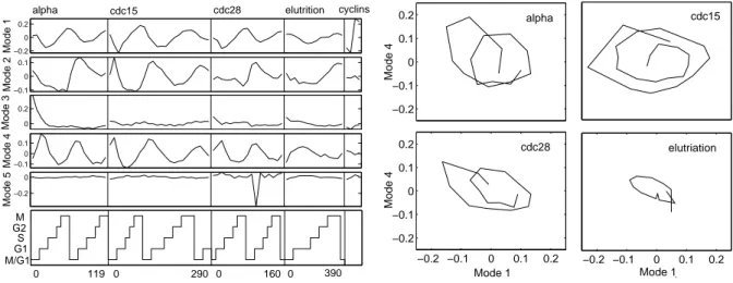
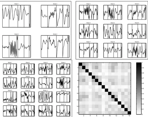
![Figure 2.7: Estimation of gene programs from the cell stress data set Causton et al. [10].](https://thumb-eu.123doks.com/thumbv2/1library_info/5598985.1691024/46.892.191.733.265.715/figure-estimation-gene-programs-cell-stress-data-causton.webp)
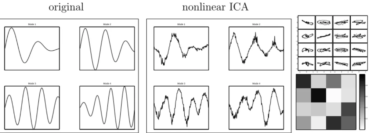
![Figure 3.4: Gene programs from the stress response data Gasch et al. [32], determined by nonlinear ICA](https://thumb-eu.123doks.com/thumbv2/1library_info/5598985.1691024/50.892.140.786.293.743/figure-gene-programs-stress-response-gasch-determined-nonlinear.webp)
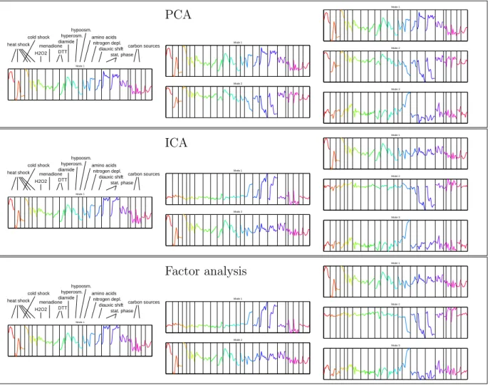
![Figure 4.5: ICA of cell cycle data [107]. Left: Sorting the 76 independent components.](https://thumb-eu.123doks.com/thumbv2/1library_info/5598985.1691024/61.892.134.792.172.406/figure-ica-cell-cycle-left-sorting-independent-components.webp)