IHS Economics Series Working Paper 284
February 2012
Marketing Response Models for Shrinking Beer Sales in Germany
Wolfgang Polasek
Impressum Author(s):
Wolfgang Polasek Title:
Marketing Response Models for Shrinking Beer Sales in Germany ISSN: Unspecified
2012 Institut für Höhere Studien - Institute for Advanced Studies (IHS) Josefstädter Straße 39, A-1080 Wien
E-Mail: o ce@ihs.ac.atffi Web: ww w .ihs.ac. a t
All IHS Working Papers are available online: http://irihs. ihs. ac.at/view/ihs_series/
This paper is available for download without charge at:
https://irihs.ihs.ac.at/id/eprint/2119/
Marketing Response Models for Shrinking Beer Sales in Germany
Wolfgang Polasek
284
Reihe Ökonomie
Economics Series
284 Reihe Ökonomie Economics Series
Marketing Response Models for Shrinking Beer Sales in Germany
Wolfgang Polasek February 2012
Institut für Höhere Studien (IHS), Wien
Institute for Advanced Studies, Vienna
Contact:
Wolfgang Polasek
Department of Economics and Finance Institute for Advanced Studies Stumpergasse 56
A-1060 Vienna, Austria
: +43/1/599 91-155 email: polasek@ihs.ac.at and
CMUP, Porto
Founded in 1963 by two prominent Austrians living in exile – the sociologist Paul F. Lazarsfeld and the economist Oskar Morgenstern – with the financial support from the Ford Foundation, the Austrian Federal Ministry of Education and the City of Vienna, the Institute for Advanced Studies (IHS) is the first institution for postgraduate education and research in economics and the social sciences in Austria. The Economics Series presents research done at the Department of Economics and Finance and aims to share “work in progress” in a timely way before formal publication. As usual, authors bear full responsibility for the content of their contributions.
Das Institut für Höhere Studien (IHS) wurde im Jahr 1963 von zwei prominenten Exilösterreichern – dem Soziologen Paul F. Lazarsfeld und dem Ökonomen Oskar Morgenstern – mit Hilfe der Ford- Stiftung, des Österreichischen Bundesministeriums für Unterricht und der Stadt Wien gegründet und ist somit die erste nachuniversitäre Lehr- und Forschungsstätte für die Sozial- und Wirtschafts- wissenschaften in Österreich. Die Reihe Ökonomie bietet Einblick in die Forschungsarbeit der Abteilung für Ökonomie und Finanzwirtschaft und verfolgt das Ziel, abteilungsinterne Diskussionsbeiträge einer breiteren fachinternen Öffentlichkeit zugänglich zu machen. Die inhaltliche Verantwortung für die veröffentlichten Beiträge liegt bei den Autoren und Autorinnen.
Abstract
Beer sales in Germany are confronted for several years with a shrinking market share in the market of alcoholic beverages. I use the approach of sales response function (SRF) models as in Polasek and Baier (2010) and adapt it to time series observation of beer sales for simultaneous estimation. I propose a new class of growth sales (gSRF) models having endogenous and exogenous variables as in Polasek (2011) together with marketing efforts that follow a sustained growth allocation principle. This approach allows to model growth rates in markets that are exposed to fierce competition and where marketing efforts cannot be evaluated directly. The class of gSRF models has the property that it models supply (i.e.
marketing efforts) and demand factors jointly in a log-linear regression model that are correlated over time. The estimated model can explain the relative success of marketing expenditures for the shrinking beer market in the period 1999-2010.
Keywords
Sales response functions (SRF), marketing budget models, MCMC estimation, beer consumption, optimal budget allocation
JEL Classification
C11, C15, C52, E17, R12
Contents
1 Introduction 1
1.1 Other approaches to beer marketing ... 1
2 Some remarks on SRF models and their estimation 2
2.1 Stochastic partial derivatives (SPD) in a sales model ... 3
3 The SRF(1) model with optimal allocations (OA) 4
3.1 The SPD condition for SRF(1) models ... 6 3.2 MCMC estimation in the SRF(1)-OA model ... 7
4 The AR-SRF(1)-OA model with SPD 9
4.1 A loss function for growth rates ... 10 4.2 MCMC estimation in the AR-gSRF(1)-OA model ... 11
5 Example: Ads and beer consumption in Germany 13
5.1 Results for the AR-SRFX model ... 13
6 Conclusions 15
References 17
7 Appendix 17
7.1 Proof of Theorem 1 (MCMC in the SRF-OA model) ... 17 7.2 The griddy Gibbs sampler ... 19
Marketing response models for shrinking beer sales in Germany 1
1 Introduction
Beer consumption and production in Germany is an important economic ac- tivity but has declined over the last decade. Therefore it is rather surprising that regional beer consumption is not available as a panel data set from the German statistical office. Only marginal data, like the total beer production or the total marketing effort per year is available. This incomplete data base was the starting point of this paper: Is it possible to make inference in a short time series model even if detailed information across regions is missing and the marketing strategies of the many (regional) beer companies are not known?
Kao et al. (2005) have proposed a simultaneous estimation of marketing success in dependence of optimal inputs in a sales response function (SRF) model. The main idea behind this approach is that the (optimal) expendi- tures for inputs might depend on the current sales and should be estimated endogenously.
Polasek (2010) has introduced a family of multiplicative SRF(k) for a cross- sectional sample where the parameterkdenotes the number of input variables (sales expenditures and sales related covariates) that are producing the sales output by a Cobb-Douglas type of production function. The multiplicative model is extended to an additive SRF(k) model and a semi-additive SRF(k) model, where we have a mixture of additive and multiplicative input terms.
The current approach emphasizes the system approach of the demand- supply system for the estimation of a SRF in a panel model, because the input variables (marketing efforts) are jointly determined by the output (sales). This approach is the focus of macroeconomics and developed in econometrics since several decades. New is the assumption that the endogeneity of the inputs stem from an implied (stochastic) optimality consideration, which is imposed through a first derivative constraint.
The paper is laid out as follows. In the next section 2 we justify our ap- proach to sales response models by some general considerations. In section 3 we describe the basic SRF(1)-SPD model and the estimation approach. Sec- tion 4 extends this approach to SRF(1)-AR models, since we have to expect in time series models auto-correlated errors. In section 5 we discuss the Example for the German beer market and the final section concludes.
1.1 Other approaches to beer marketing
There are almost no studies that try to quantify the impact of advertise- ment on beer sales, also not on an international comparison. This might change if the beer industry becomes a more global player and has to mar- ket beer brands internationally. If there are more mergers and acquisitions, then this will change the marketing strategies. In an article of ’Marketwatch’
(http://www.marketwatch.com/story/inbev-takeover-spotlights-anheuser-buschs- big-ad-budget) we find the following quote in reaction to the takeover of Anheuser-Busch: ”Will sports lose one of its biggest boosters? InBev takeover
2 Wolfgang Polasek
spotlights Anheuser-Busch’s big ad budget. . . . That leaves Anheuser-Busch’s massive advertising and sponsorship budget perhaps the juiciest target of swift cost-cuts.
The No.1 U.S. beer maker is the nation’s 22nd largest advertiser, according to data compiled by Advertising Age and TNS Media Intelligence, with total expenditures of $1.36 billion last year. About a third of that – $475 million – is spent on TV, radio, magazines and the Internet, with the rest aimed at trade promotions, sponsorships, point-of purchase ad space and the like.
By contrast, SAB-Miller spent $230 million on U.S. media last year and Di- ageo, the world’s largest spirits company with revenues in excess of Anheuser- Busch’s, laid out $173 million. . . . ”
Thus, in the aftermath of market concentration, new strategies on spending ad budgets will be developed. This will also affect the sponsoring market, as the following quote on the same web site shows:
”Will sports lose its biggest ad booster? . . . How will InBev’s $52 billion takeover of Anheuser-Busch affect the No. 1 U.S. brewer’s massive sports advertising and sponsorship budget?”
2 Some remarks on SRF models and their estimation
A shrinking sales market like the German beer market is challenge for quanti- tative marketing models. The recent class of sales response models that were promoted by Kao et al. (2005) and Baier and Polasek (2010) provide a flexible framework to estimate by MCMC models the reaction of marketing efforts in such markets. Models for sales response functions (SRF) provide a class of models that can be combined with many additional assumptions on the re- lationship between the supply and demand side of the market. For example, in cross-sections or panels, the SRF model can be extended to the SRF-SAR model, where SAR stands for a spatial autoregressive model (see e.g. Anselin 1986), as will be shown in a next paper.
Common to all approaches is that they assume a behaviorial model for sales and marketing actions and therefore an appropriate joint model for the demand and the supply side has to be found. The supply side model is gov- erned by an market strategy that follows some optimality principle. For the shrinking beer market we have assume a new sustained optimal growth alloca- tion principle that results in an allocation rule that sales expenditures follow a constant rule that is proportional to the first partial derivative over time.
Since this variable cannot be observed directly we need to assume a latent variable.
The estimation of the latent variable SRF model for the German beer market shows that there has been some positive effects of beer marketing expenditures to fight the shrinking markets that was mainly caused by the increasing market share of the wine sales in the German alcoholic beverage market. Therefore we need to estimate an SRF(1)X(1) model where the X
Marketing response models for shrinking beer sales in Germany 3 stand for the exogenous (control) variable, in our case the increasing wine share in the market.
For this shrinking sales over time we suggest to use a multiplicative SRFX model applied to growth factors, briefly denoted by gSRFX model. Also we cannot use the Albers marketing allocation rule as a response of the supply side, since no regional data are involved. Instead we suggest that the supply side follows a sustained growth allocation rule of the marketing expenditures, such that a simple allocation rule follows. In such behaviorial models it is not necessary to assume that marketing strategist will do in practice these mathematical calculations, rather we like to know if such a combination of simple SRF models and observed marketing expenditures lead to a simultane- ous model of right and left hand side variables that explains the reality better.
Because of the complexity of the parameters involved and the usually small data base it seems that MCMC methods work best at the moment to achieve this goal.
2.1 Stochastic partial derivatives (SPD) in a sales model
If the first derivative of a sales response (SRF) model is used as a latent vari- able then the sales equation (log-y equation) and the derivative equation imply a simultaneous equation system, and the stochastic allocation restriction im- ply an endogeneity of the single input variablex. The following 3 stochastic assumptions are the basic building blocks for the SRF-SPD model and are based on 3 types of considerations that reflect the interaction of the actions observed in the market from the demand and the supply side that leads to appropriate steps (= equations) in the joint model building process:
1. The stochastic (demand) model: input variables and the func- tional form imply (⇒) output variables plus noise.
2. The allocation model (supply side): Stochastic response model + imposing optimal expenditure allocations = input variables & func- tional form (SRF)⇒first derivatives plus noise.
3. The final model (conditional on assumed demand and supply re- sponses): Known SRF coefficients & SPD assumptions ⇒ stochastic regressors (pivotal variable change).
The sales response model that assumes stochastic SPD allocations implies the following additional (implicit) assumptions that are part of the estima- tion process:
1. The ”stochastic ads allocation” rule: We assume that the realized derivatives of sales w.r.t. marketing efforts are approximately equal. We use the concept of realized derivatives to emphasize the fact, that the exact sales changes are unknown and have to be estimated for the estimation of the model by the first derivatives, which is model dependent, i.e. depends on the assumed functional
4 Wolfgang Polasek
form of the SRF. The company management have learned in the past to un- derstand and to know about the SRF function in their field, even if the exact functional form is unknown to them. Therefore they use the input variables in an optimal way, that is they look to spend promotional money in such a way that for each region the change in sales is about equal.
2. This implied behavioral assumption of the SRF model has to be incorpo- rated into the estimation process and leads to a larger model class of system estimation, since the input and output variables (y and x) are endogenously linked by this assumption.
3. Thus the SDP assumption (for ads allocations) implies a joint distribution of all the endogenous variables, since the realized derivatives depend on the functional form of the SRF model.
4. The derivative w.r.t. marketing expenditures cannot be directly observed (either the amount channeled through the input variables is unknown or the sales changes are not reported on this disaggregated level or is imprecisely measured). Thus, it becomes necessary to introduce the unobserved deriva- tive as a latent variable in the estimation process.
5. In the MCMC estimation procedure the latent derivatives are generated by so-called ’direct simulations’ from the current specification of the SRF model.
6. The latent variable can be viewed as a proxy variable, which is simulated through a model that uses the exogenous regressors of the system.
In the next section we introduce the SRF(1) model and the MCMC estimation under the SPD assumption.
In Section 5 we discuss a regional sales response model that involves data from the German beer market for the period 1997 to 2010. In a final section we conclude.
3 The SRF(1) model with optimal allocations (OA)
In this section we start with the simple SRF(1) model because we want to demonstrate the consequences of the OA and SPD assumption for the esti- mation procedure.
We consider the SRF(1) sales response function y = y(x) with one input variablex
y=β0 xβ1 e, (1)
whereis assumed to be aN[0, σy2] distributed error term. By taking logs for the n cross-sectional observations we find the following linear regression model
ln y∼ N[µy =Xβ, σy2In] (2) with the regression coefficientsβ= (ln β0, β1) and the regressor matrixX = (1n : ln x) where 1n is a vector of 1’s and x is the cross-sectional decision
Marketing response models for shrinking beer sales in Germany 5 variable that will influence the salesy(an×1 vector) in the n regions. Thus the model is of the type of a log linear production function as it is used in macro-economics.
For the optimal allocation problem in SRF models we need a target func- tion that is suitable for sustainable growth rates.
Definition 1 (The stochastic allocation rule for ads expenditures).
We assume positive (and uncorrelated) salesyi, i= 1, ...., noverntime periods and we assume that the total budget Btot is allocated optimally over the n periods. The profit function to be maximized is P =Pn
i=1diy(xi). di is the marginal contribution of the product to the profit. Since we only considering 1 product, we can set di= 1. This leads to the following Lagrange function:
n
X
i=1
diy(xi) +λ(Btot−
n
X
i=1
xi)
The solution of this optimal allocation problem is given by setting the first derivative to zero, from where we find
di∂y/∂xi∝(yx)i =λ f or i= 1, ...., n, (3) or that all derivatives of the salesy(xi)w.r.t. the marketing effortxi have to be constant. In cross-sections we refer to this ’stochastic allocation’ rule (better described as optimal allocation rule plus stochastic behavioral assumption) as
’Albers’ rule because of Albers (1998).
This leads to the basic multiplicative (or Cobb-Douglas) type SRF model:
Definition 2 (The SRF model with latent partial derivatives). For observed regressorx, the multiplicative SRF(1) modely=β0 xβ1 e is defined as the following set of 2 log-normal densities:
ln y∼ N[ln β0+β1ln x, σ2yIn]
ln yx∼ N[log(β0β1) + (β1−1)ln x, σy2In] (4) where yx is the first derivative of the SRF(1) model and with the parameters of the model given by θ= (β, σy2).
Note that this is a non-linear model inβ and also a very restricted model, since the sales observations y and the derivatives yx follow normal distribu- tions with the same variance. Furthermore, both equations are correlated and cannot be jointly estimated if yx is unobserved. Thus, we need to look for better modeling strategies.
6 Wolfgang Polasek
3.1 The SPD condition for SRF(1) models
We obtain an alternative SRF(1) model if we combine the assumptions for generating the first derivatives ˙y = ln yx of the SRF model via the latent variable and the assumption of a stochastic optimal allocation (OA) rule like the stochastic Albers rule, like ˙yi= (ln yx)i
˙
yi|θλ∼ N[λ, σλ2] f or i= 1, ..., n (5) or ln yx ∼ N[λ1n, σ2λIn]. This means that the sales responses y and the decision variable ximply a prescription that marketing resources should be allocated according to the first derivative of the SRF model. Since the empir- ical observations across the nregions reveal some noise, we assume that the
˙
yi’s are independently normally distributed for given parametersθλ= (λ, σλ2).
These stochastic fluctuations of the derivatives across thenunits are captured by the mean response λ, and the varianceσ2λ in assumption (5) imposes the looseness or strength of this target λ, the optimal behavior, from the actual but not observed derivativesyx. It measures in practice how good marketing people follow the prescription of the optimal allocation (OA) model.
If the ˙y’s could be observed, there would be no extra stochastic dependen- cies. In our model we have to proxy the unobserved derivatives by the realized derivatives of the multiplicative SRF function in (5):
˙
y=Xβe with βe=
ln(β0β1) β1−1
(6) Adding this stochastic partial derivative (SPD) constraint for thexregres- sor in the SRF model creates an behaviorial model that the partial derivatives should be (approximately) equal across the regional units:
Lemma 1 (The SPD assumption for the SRF(1) model).
The combination of the stochastic optimal allocation (OA) rule (5) and the generation of the latent partial derivatives as in (4) implies the endogene- ity of x in the SRF(1) model. Thus, the SPD assumption implies a normal distribution of the regressorxin the following way:
ln x|θλ∼ N[µx(θλ), σx2(θλ)], (7) with the parameters θλ= (λ, σλ2)and mean and variance
µx= ln(β0β1)−λ
1−β1 , σ2x= σ2λ
(β1−1)2 (8)
Proof. There are several ways to derive the result. One leads via the trans- formation rule for random variables to the Jacobian ofln xis just 1/|β1−1|.
The other approach just equates equations (5) and (4) and solves forln(x).
One way to see how the SPD assumption translates to an assumption about thexis to write the exponent of the density (5) and use the log derivative (4)
Marketing response models for shrinking beer sales in Germany 7
(ln yx−λ)2/σλ2 = (ln(β0β1) + (β1−1)ln x−λ)2/σ2λ=
=
log(β0β1)−λ 1−β1
−ln x 2
(β1−1)2/σλ2
∝p(ln x|µx, σ2x)
Finally, we can define the SRF(1)-OA and the SRF(1)-SPD model in the following way:
Definition 3 (The SRF(1)-SPD model).
(a) The SRF(1)-SPD model is based on the multiplicative SRF model y = β0 xβ1 e, the endogeneity of xand the stochastic Albers rule (Definition 1), which result in the following set of 3 log-normal densities:
ln y |θy ∼ N[ln β0+β1ln x, σ2y]
⇒ln x|θλ ∼ N[(ln β0+ln β1−λ)/(β1−1), σ2λ/(β1−1)2]
ln yx|θλ ∼ N[λ, σλ2], (9)
where yx is the first derivative of the SRF(1) model and is considered as a latent variable. The parameters of the model are given by θ = (β, λ, σy2, σ2λ) and θλ= (λ, σ2λ), θy = (β, σ2y). The ”⇒” denotes the derived distribution for ln x, making the SPD and the constant allocation assumption.
(b) The SRF(1)-OA modelthat generates the endogeneity ofxindirectly, and leads to the following reduced set of equations, with the restrictionβ1>0
ln y|θy ∼ N[ln β0+β1ln x, σ2y]
ln yx|θλ ∼ N[λ, σλ2]. (10)
Again, ln yx=Xβeis the realized derivative (6), and thus just a linear trans- formation of the regressorsX and theβ coefficients,and therefore for the con- trol variable x, say a+bx. Therefore, this stochastic OA assumption implies implicitly a distribution for x.
For statistical inference we can estimate the parameter vector by maximum likelihood or by MCMC, assuming a prior density given byp(θ). In the next section we outline the MCMC procedure.
3.2 MCMC estimation in the SRF(1)-OA model
This section develops the MCMC estimation for the SRF(1)-OA model. The optimal allocation (OA) rule in the SRF model requires a first derivative, which can be not observed by data, and therefore has to be introduced into the model as a latent variable.
The latent variable defines another equation in the D/S system that can be generated conditionally through the assumptions of the system. The latent
8 Wolfgang Polasek
variable ˙y=ln yxis considered to be a homolog (i.e. over-parameterized) pa- rameter vector that is computed or estimated from the demand or y-equation.
Finally, the observed data D= (ln y, ln x) and the latent variableln yx are modeled by the joint density p(ln y, ln x, ln yx), which decomposes in the general case as
p(ln y|ln x, β, σ2x, ...)p(ln x|β, ln yx, ...)p(ln yx|λ, σ2λ∗, ...).
Because the realized derivative ln yx =Xβewith X = (1n : x) is generated directly as a linear combination of the x variable, the density for ln x in (11) implies a likelihood function forx. This leads to the following likelihood function for the SRF(1)-OA model
l(θ| D) =N[ln y|µy, σ2yIn]N[ln x|µx, σλ2In] (11) with the conditional means
µy =ln β0+β1ln xandµx= (ln β0+ln β1−λ)/(β1−1). (12) The prior density forθ= (β, σy−2, σλ−2) is
p(θ) =N[β|β∗, H∗]N[λ|λ∗, σλ∗2 ]N[ln yx|λ, σλ2] Y
j∈{y,λ}
Ga[σj−2|σ2j∗, nj∗].
(13) Thus, the SRF(1)-OA model consists of
1. The prior density (13), 2. The likelihood function (11), 3. The realized derivative (6).
The posterior distributionp(θ| D)∝l(D |θ)p(θ) is simulated by MCMC.
Theorem 1 (MCMC in the SRF(1)-OA model).
The MCMC iteration in the SRF(1)-OA model with the likelihood function (11) and the prior density (13) takes the following draws of the full conditional distributions (fcd):
1. Starting values: set β=βOLS andλ= 0 2. Drawσ−2y fromΓ[σy−2|s2y∗∗, ny∗∗] 3. Drawσ−2λ fromΓ[σλ−2|s2λ∗∗, nλ∗∗] 4. Drawλfrom N[λ|λ∗∗, s2λ∗∗]
5. Compute the current derivative y˙ =ln yx fromN[ ˙y|µy˙,(s2y)In] 6. Drawβ = (β0, β1)from p(β0)andp(β1|β0)
7. Repeat until convergence.
Proof. The proof is given in the Appendix.
Marketing response models for shrinking beer sales in Germany 9 The marginal likelihood of modelMis computed by the Newton-Raftery formula
ˆ
m(y| M)−1= 1 nrep
nrep
X
j=1 n
X
i=1
ln l(Di| M, θj)
!−1
l(Dj| M, θ)−1 (14)
whereDi= (ln yi, ln xi) is the i-th data observation and with the likelihood given in (11).
4 The AR-SRF(1)-OA model with SPD
In this section we describe the AR-SRF model because we want to demonstrate the effects of correlated time series for the estimation procedure. The AR- SRF(1) sales response function with one input variables x and the lagged endogenous variabley−1is
y=β0yρ−1xβ1e, or
ln y=ρ ln y−1+ln(β0) +β1ln x+, (15) where is aN[0, σ2y] distributed error term. This leads to the reduced form equation
Rln y=ln y−ρln y−1=ln(β0) +β1ln x+ with
R=In−ρL with L=
0 1 0 ...
0 0 1 0 ...
0... ... 0 1 0 0 ... 0
(16)
and Lbeing a supra-diagonal or the AR(1) lag-shift matrix. By taking log’s for thenobservations we find for knownρthe reduced form regression model for the generalized differences
R ln y∼ N[ln(β0) +β1ln x, σ2yin], (17) The mean of the reduced form regression for the generalized differences Rln y = ln y−ρln y−1 is µy = Xβ with coefficients β = (ln β0, β1) and the regressor matrixX = (1n:ln x) is given as before, where 1nis a vector of 1’s andxis the supply-side control variable that will influence the salesy (a n×1 vector). Thus, the model is again a log-linear production function as it is used in macro-economics. The stochastic partial derivative (SPD) assump- tion is applied to the reduced form equation (17) and leads to the behavioral equation
˙
g=∂Ry/∂x=β0β1 xβ1−1 e. The realized first derivative is
10 Wolfgang Polasek
gx= ∂Ry
∂x |x:n×1
evaluated at the vectorx. This log (realized) derivative, for knownβand SRF, is given as in the simple SRF model (18) by
ln gx=µg˙ +=ln(β0β1) + (β1−1)ln x+, (18) and therefore the log derivative p(ln gx | β, x) = N[µg˙, σy2In] with µg˙ = ln(β0β1) + (β1−1)ln xis normally distributed.
This leads to the following AR-SRF(1)-OA (optimal allocation) model:
Definition 4 (The AR-gSRF(1)-OA model with the partial deriva- tive as a latent variable).For observedy andxthe the AR-gSRF(1) model (in reduced form) is defined with R as in (16) andβ1>0 as the following set of 2 log-normal densities:
Rln y∼ N[ln β0+β1ln x, σ2yIn]
ln yx∼ N[ln(β0β1) + (β1−1)ln x, σy2In], (19) whereyxis the first derivative of the AR-gRF(1)-OA model andθ= (β, ρ, σy2) are the parameters of the model.
4.1 A loss function for growth rates
We consider the growth factor over time and we argue that the growth factors are the target of the SRF models to monitor long term sales growth. The growth rates are obtained from the growth factors by taking logs.
The total budget available is Btot and instead of maximizing the profit directly, we look for a function that maximizes the sustainable growth of sales. Thus, the criterion to be maximized is slightly different:
Q=
n
X
i=1
gt(xi) where gt(xi) = yt(xi) yt−1(xi).
gt(xi) denotes the growth factor of the sales: The growth factors are needed to ensure positive vales of the SRF model. This function is correlated with the profit function in (1). As a side constraint we assume that the company is interested in a sustainable growth path, which is expressed as deviation between the average growth rate
¯ g= 1
n
n
X
i=1
gt (20)
from a target growth rateg∗overnperiods. These considerations lead to the following optimisation problem using the Lagrange function for the growth factors of sales, which mimics the Albers rule (1) for a time period of length n:
Marketing response models for shrinking beer sales in Germany 11 Definition 5 (An optimal allocation (AO) rule for sustainable growth).
We consider the growth factorsgt(xi)of sales that depend on the ads variable xfornperiods and we assume that the ads expenditures are allocated according to a sustainable growth path as in (20)
G(xi, λ) =
n
X
i=1
gt(xi) +λ(ng∗−
n
X
i=1
gt(xi)). (21) The solution of this Lagrange problem requires setting the first derivative
∂G/∂xi to zero, from where we find
gx=∂gt/∂xi=λ f or i= 1, ..., n, (22) or that all derivatives of the sales growth factors gt(xi) w.r.t. the marketing effortxi have to be constant.
While the Albers rule is applicable for sales innregions, the sustainable growth rule works for time series. It is set up in a similar way so that we have a simple ads allocation rule over time. Note the similarity to the original stochastic Albers rule. If a long-term planing horizon and the budget becomes important, then the cross-sectional units are replaced by time series data.
Thus, the ads budget can be allocated in a simple way over the planing period.
4.2 MCMC estimation in the AR-gSRF(1)-OA model
This section develops the MCMC estimation for the AR-gSRF(1)-OA model, defined in 4. The likelihood function the parameters θ = (β, σ−2y , λ, ρ) is a function of the observed dataD
l(θ| D) =N[Rln y|µy, σ2yIn] (23) with the conditional meanµy
µy =ln β0+β1ln x (24)
Because the latent variableln yx can be realized derivativeln yx=Xβewith X = (1n :x) is generated directly as a linear combination of the xvariable, the second density in (23) tranlates actually to a likelihood function for x.
The prior density forθis
p(θ) =N[β|β∗, H∗]N[λ|λ∗, σ2λ∗] Y
j∈{y,λ}
Ga[σ−2j |σj∗2 , nj∗] (25)
where all the parameter with a ’*’ index denote known hyper-parameters of the prior distribution. Finally, the AR-gSRF(1)-OA model consists of
12 Wolfgang Polasek 1. The prior density (25), 2. The likelihood function (23), 3. The realized derivative (6).
The posterior distributionp(θ| D)∝l(D |θ)p(θ) is simulated by MCMC.
Theorem 2 (MCMC in the AR-gSRF(1)-OA model).
The MCMC iteration in the AR-gSRF(1)-OA model with the likelihood func- tion (23) and the prior density (25) takes the following draws of the full con- ditional distributions (fcd):
1. Starting values: set β=βOLS andλ= 0 2. Drawσ−2y fromΓ[σy−2|s2y∗∗, ny∗∗] 3. Drawλfrom N[λ|λ∗∗, s2λ∗∗] 4. Computeg˙ =ln gx=Xβe
5. Drawβ = (β0, β1)from p(β0)andp(β1|β0) 6. Drawρby a griddy Gibbs step using p(ρ| D, ...).
7. Repeat until convergence.
Proof. The proof is almost identical to Theorem 1, except that we need one more fcd for the extra parameter ρ. Furthermore only the fcd’s for the first layer for the log-y equation, β and the residual variance are affected by the reduced form transformation y → Ry: The residuals in (33) change to ey = Rln y−Xβ and the fcd (29) forβ changes to
p(β | D, ...)∝N[β|β∗, H∗]N[R ln y|Xβ, σ2yIn]N[ln x|µx, σ2λ/(1−β1)2In] (26) and we have to make the variable change in (30) to
b#=H#
H∗−1b∗+σ−2X0Ry .
For the fcd of the correlation coefficientρwe find a univariate normal distri- bution that can be easily evaluated based on the simple OLS estimate ofρ. The fcd is proportional to
p(ρ) =p(ρ| D)∝σy−2Texp
− 1
2σ2(Ry−I†τ)0(Ry−I†τ)
.
I† is the row-truncated identity matrixIn, that adjusts for thek < nparam- eters inτ. (For second order smoothnessk=n−2.) The griddy Gibbs step is surprisingly simple as follows. We evaluate a grid of 100ρ-points around the OLS estimate of the normal linear model that follows from the fcd for rho:
y=ρLy+. Under normality we have
ρ∼ N[ ˆρ, σρ2] with ρˆ=y0Ly/y0L0Ly and σρ2=σy2/y0L0Ly.
This follows because the exponent is (y−ρy−1)0(y−ρy−1)/σ2 = (ρ− ˆ
ρ)2Sy/σ2y∝ N[ρ|ρ, σˆ 2y/Sy].
Marketing response models for shrinking beer sales in Germany 13 Note that the MCMC algorithm for the AR-gSRF-X model parallels the structure in Theorem 2, only the variables in the regressor matrix have to be arranged as X = (1 :z:x), in blocks of exogenous and endogenous variable wherez is the exogenous variable.
Model choice: The marginal likelihood of modelMis computed by the Newton and Raftery (1994) formula (14) with the likelihood given in (23).
5 Example: Ads and beer consumption in Germany
The German beer sales in hekto-liter (hl) and the marketing expenditures (in mio Euros) for 1997-2010 are found in Table 1. (Source: The German Statistische Bundesamt)
Table 1: German beer and ads data 1997-2010 Year Sales (hl) Marketing
1997 103 402,00 1998 100,18 431,00 1999 110,10 380,00 2000 109,80 388,00 2001 107,80 360,00 2002 107,80 347,00 2003 105,60 331,00 2004 105,90 364,00 2005 105,40 410,00 2006 106,80 374,70 2007 104,00 399,30 2008 102,90 401,80 2009 100,00 350,30 2010 98,30 376,88
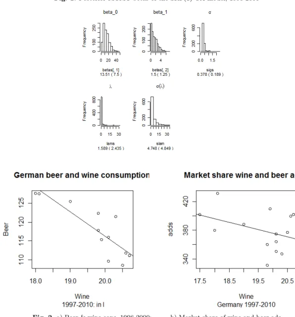
The MCMC densities of the parameters of the SRF(1)-OA model are in Figure 1.
The connection between beer and wine consumption is quite strong, as we see in Figure 2.a) but there is also a surprising negative correlation between the market share of wine and beer ads (in Euros) in Germany.
5.1 Results for the AR-SRFX model
The log data of the SRF(1)X(1)-AR(1) model are displayed by a scatter-plot matrix with bivariate regression lines in Figure 3.
The modeling strategy is as follows. We start with the most complex model as its MCMC estimation is given for the AR-SRFX-AO model in Theorem 2. Also, because of negative MCMC diagnostics, we dropped the assumptions of a model imposing a SPD prior for the control variablexand we prefer to use the SRFX-AO model. Furthermore, we prefer for the σλ−2 parameter to be fixed at a tight constant, implying that the (stochastic) sustainable growth allocation rule is taking place in a rather tight narrow band. Based on the
14 Wolfgang Polasek
Fig. 1. Posterior MCMC betas of the SRF(1)-OA model, 1998-2000
Fig. 2.a) Beer & wine cons. 1998-2000; b) Market share of wine and beer ads
OLS estimate of ρ, theσ−2λ can be easily fixed at the variance of the latent variableln y=yx evaluated at the OLSβ coefficients.
The MCMC estimates of the AR-SRF model are:
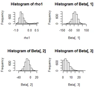
mean beta SD beta beta[1] 7.7093 30.1995 beta[2] -11.4056 8.2757 beta[3] 5.0096 3.4994
Marketing response models for shrinking beer sales in Germany 15 Fig. 3.The log data for SRFX-AR model in Germany 1999-2010
For the auto-correlation coefficient we find as average over the MCMC sampleρ=−0.5089, SD(ρ) = 0.2873.
The density estimates can be seen in Figure 4. Convergence was achieved very fast and the use of the griddy Gibbs method created no autocorrelation in the ρ-runs. (A Metropolis-Hastings algorithm did not work so well.) The range of coefficients is rather wide, but this is not surprising since there are only 12 observations. (Classical results based on asymptotic distributions would not work well for this data set.) The elasticity on log ads (the endogenous vari- able) has to be positive which is the case in 75% of the number of iterations.
Interestingly, by discarding the negative draws, we get about the same type of distributions (histogram shapes) of the coefficients.
Following our ”general to more simpler” specification philosophy we find, that fixing certain hyper-parameters at a reasonable value yield better estima- tion results for the coefficients of the SRF model in the first stage. The crucial parameter is λandλ∗. Further research is needed on how big this sensitivity is and how big the stochastic relaxation of the optimal allocation rule can be. Because there are many parameters to estimate plus a latent variable, the Bayesian analysis improves if there are fewer ’free’ parameters to estimate.
6 Conclusions
The paper has shown that the class of sales response models is large and flexible enough to cope with shrinking sales in sales models with advertisement expenditures. The results of the sales growth response function (gSRF) model
16 Wolfgang Polasek
Fig. 4. The density estimates for SRFX-AR model in Germany 1999-2010
point in the right direction, but only if important possible marketing behaviors have been appropriately implemented in the model.
As an additional consideration for the estimation of an SRF model in a time series context we have proposed a specification that allows for AR(1) errors. With this assumption we leave the framework of easy simulations in the MCMC algorithm using normal and gamma distributions. We found that the use of the griddy Gibbs sampler for the autocorrelation coefficients leads to a quick mixing of the sampler without the perils of long autocorrelation when a Metropolis-Hastings step is used.
Given the large variety of models (SRF-X and AR-SRF-X) we have tried and from the non-significant estimation results we conclude that the beer industry has not reacted in a proper way to fight the shrinking sales in the beer market in Germany over the last decade. For future work, many further extensions of this flexible class of SRF-X models are possible. First of all there is the ques- tion of the right or appropriate functional form of the SRF-X class models.
following the suggestions of Kao et al. (2005) more research is needed, espe- cially if time series and shrinking markets have to be considered. Secondly, there is the question of the appropriate marketing actions and strategies un- dertaken by the supply side of the market.
A possible next step for a better model choice is the use of Bayesian model av- eraging (BMA) techniques. Thus, there is room for more theory as how market participants react either as consumers to marketing efforts or as marketing strategists who react either to sales developments or company policies. Sys- tem estimation would be required if more than 1 marketing channels should
Marketing response models for shrinking beer sales in Germany 17 be optimized or if marketing efforts depend also on the sales performance of the competitors.
References
1. Albers S. (1998) Regeln fuer die Allokation eines Marketingbudgets auf Produkte oder Marktsegmente, Zeitschrift fuer Betriebswirtschaftliche Forschung50, 211- 229.
2. Anselin L.(1988) Spatial Econometrics. In: B. H. Baltagi (Ed.),A Companion to Theoretical Econometrics. Blackwell Publishing Ltd AD, 310–330.
3. Baier D., and Polasek W. (2010), Marketing and Regional Sales: Evaluation of Expenditure Strategies by Spatial Sales Response Functions, in: Studies in Classification, Data Analysis, and Knowledge Organization, Vol. 40, 673-682.. 4. Kao L.-J., C.-C. Chiu, T.J. Gilbride, T. Otter, and G.M. Allenby (2005) Evalu-
ating the Effectiveness of Marketing Expenditures. Working Paper, Ohio State University, Fisher College of Business.
5. Newton M.A., and A. E. Raftery (1994) Approximate Bayesian inference with the weighted likelihood bootstrap (with discussion). Journal of the Royal Statistical Society, Series B, 56, 3-48
6. Polasek W. (2010a), Sales Response Functions (SRF) with Stochastic Derivative Constraints, Institute fuer hoehere Studien, Wien.
7. Polasek W. (2010b), Endogeneity and Exogeneity in Sales Response Functions, to appear in GFKL 2010.
8. Polasek W. (2011), Multi-level panel models for regional beer sales in Germany, Institute fuer hoehere Studien, Wien.
9. Ritter Ch., and Martin A. Tanner (1992), Facilitating the Gibbs Sampler: The Gibbs Stopper and the Griddy-Gibbs Sampler, Journal of the American Statis- tical Association, Vol. 87, No. 419, 861-868
10. Rossi P.E., G.M. Allenby, and R. McCulloch (2005) Bayesian Statistics and Marketing. John Wiley and Sons, New York.
7 Appendix
7.1 Proof of Theorem 1 (MCMC in the SRF-OA model) Proof. The full conditional densities (fcd’s) are as follows:
1. The fcd for λ, the average utility level can be estimated in the same way as before:
p(λ| D, ...)∝ N[λ|λ∗, s2λ∗]N[ln yx|λ1n, σλ2In]∝ N[λ|λ∗∗, s2λ∗∗] (27) withs−2λ∗∗=s−2λ∗+nσ−2λ and from (5) we find in the exponent the quadratic from (ln yx−λ1n)0σλ−2(ln yx−λ1n)
λ∗∗ =s2λ∗∗(s−2λ∗λ∗+nσ−2λ 10n(ln yx)),
whereσ2λ is the variance ofyx and the realized yx’s are evaluated at the currentβ.
18 Wolfgang Polasek
2. The fcd for z=ln yx under SPD is
p(ln yx| D, ...)∝ N[ln yx|µz, σz2In]N[ln yx|λ1n, σλ2In]
=N[z|µz∗∗, s2z∗∗In]. (28) withs−2z∗∗=σz−2+σ−2λ andµz∗∗=s−2z∗∗(s−2z µz+σ−2λ 1nλ).
3. The fcd for β coefficients is
p(β | D, ...)∝ N[β |β∗, H∗]N[ln y|Xβ, σ2yIn]N[ln yx|λ1n, σ2λIn] (29) since the third density ofln xin (29) contains theβ coefficients in a non- linear way andµx is given in (12). To avoid a Metropolis step we get a analytical solution by combining the 3 components of normal densities in 3 steps.
Step 1: The first two normal densities can be combined in the usual way to
N
β|β#= β0#
β1#
, H#=
h00h01
h10h11
with H#−1=H∗−1+σ−2X0X,
b#=H#
H∗−1b∗+σ−2X0y
, (30)
where the index ’#’ indicates an auxiliary result.
Step 2a: The conditional bivariate normal density in (30) forβ1|β0is:
p(β1|β0) =N[β1.0, σ1.02 ] with
σ1.02 =h11−h10h01/h00=h11(1−ρ201),
β1.0=β1#+h10(β0−β0#)/h00. (31) Note thatρ201is the squared correlation coefficient, defined asρ201=hh210
00h11. Step 2b: The general case for the conditional normal density in (30) for β1|β0:
p(β1|β0) =N[β1.0, σ21.0] with σ21.0=h11−h10h−100h01
β1.0=β1#+h10h−100(β0−β0#). (32) The variables in the SRF regression model need to be ordered in such a way that the component with ’0’ contains the intercept (and thezvariables of the SRFX model), while the component with ’1’ contains the endogenous variablex.
Step 3: Simulate the positiveβ1 coefficient either by keeping only those draws that are positive or draw from a truncated normal density restricted to the positive real line. The third density in (29) is also restricting the draws and follows the same drawing approach using the conditional normal
Marketing response models for shrinking beer sales in Germany 19 density. The following Metropolis-Hastings step is used: We use a random walk chain for the proposalβnew
βnew=βold+N[0, cβIk],
wherekis the dimension ofβ.cβ is a tuning constant for the variance of the proposal. The acceptance probability involves the posterior fcd density p(β=p(β | D, ...) in (29) and is given by
α(βold, βnew) =min
p(βnew) p(βold),1
,
where we accept only proposals with|β1new|>0 4. The fcd for σy−2
p(σ−2y | D, ...)∝Ga[σ−2y |σy∗∗2 ny∗∗/2, ny∗∗/2] (33) withny∗∗ =ny∗+nandny∗∗σy∗∗2 =ny∗σ2y∗+e0yey, whereey =ln y−Xβ being the current residuals of the log-y equation.
5. Only in case where the stochastic OA varianceσλ−2will be estimated: The fcd forσλ−2
p(σλ−2| D, ...)∝Ga[σλ−2|σ2λ∗∗, nλ∗∗] (34) withnλ∗∗=nλ∗+nandnλ∗∗σ2λ∗∗=nλ∗σλ∗2 +e0xex+e0λeλand the residuals ex=ln x−µxandeλ=ln yx−λ1n(ore0λeλ=P
i(ln yx,i−λ)2. This is because we have 2 variance sources
p(σλ−2| D, ...)∝
σ2λ (1−β1)2
−n/2 exp
− 1
σλ2(ln x−µx)0(ln x−µx)(1−β1)2
(σλ2)−n/2exp
− 1
σ2λ(ln yx−λ1n)0(ln yx−λ1n)
7.2 The griddy Gibbs sampler
This procedure was described in Ritter and Tanner (1992). Consider a m- dimensional posterior densityp(θ1,· · ·θm) that is estimated via MCMC and where the conditional distributionp(θi|θj, j6=i) is untractable but univari- ate. If it is difficult to directly sample from p(θi | θj, j 6=i), the idea is to form a simple approximation to the inverse cdf based on the evaluation of p(θi |θj, j6=i) on a grid of points. This leads to the following 3 steps:
Step 1. Evaluatep(θi|θj, j6=i) atθi=x1, x2, . . . to obtainw1, w2, ..., wn. Step 2. Use w1, w2, ..., wn to obtain an approximation to the inverse cdf of p(θi |θj, j6=i).
Step 3. Sample a uniform U(0,1) deviate and transform the observation via the approximate inverse cdf.
Remark 1: The functionp(θi |θj, j6=i) need be known only up to a propor- tionality constant, because the normalization can be obtained directly from
20 Wolfgang Polasek thew1, w2, ..., wn.
Remark 2: The gridx1, x2, ..., xn need not be uniformly spaced. In fact, good grids put more points in neighborhoods of high mass and fewer points in neighborhoods of low mass. One approach to address this goal is to construct the grid so that the mass under the current approximation to the conditional distribution between successive grid points is approximately constant.
Author: Wolfgang Polasek
Title: Marketing Response Models for Shrinking Beer Sales in Germany Reihe Ökonomie / Economics Series 284
Editor: Robert M. Kunst (Econometrics)
Associate Editors: Walter Fisher (Macroeconomics), Klaus Ritzberger (Microeconomics)
ISSN: 1605-7996
© 2012 by the Department of Economics and Finance, Institute for Advanced Studies (IHS),
Stumpergasse 56, A-1060 Vienna +43 1 59991-0 Fax +43 1 59991-555 http://www.ihs.ac.at
ISSN: 1605-7996