Item Response Models for the Measurement of Thresholds

Item Response Models for the Measurement

of Thresholds

A Dissertation presented to

the Faculty of the Graduate School University of Missouri-Columbia

In Partial Fulfillment

of the Requirements for the Degree of Doctor of Philosophy

by

Richard D. Morey

Dr. Jeffrey N. Rouder, Dissertation Supervisor

August 2008

The undersigned, appointed by the Dean of the Graduate School, have ex- amined the dissertation entitled:

Item Response Models for the Measurement

of Thresholds presented by Richard D. Morey

a candidate for the degree of Doctor of Philosophy

and hereby certify that in their opinion it is worthy of acceptance.

Dr. Jeffrey N. Rouder

Dr. Nelson Cowan

Dr. Paul Speckman

Dr. Lori Thombs

Dr. Douglas Steinley

ACKNOWLEDGMENTS

• Dr. Jeff Rouder, for training, help, and support over the past six years

• Mike Pratte, for his helpful discussions regarding the perils of priming paradigms

• My parents, for instilling in me a curiosity about nature and a respect for

the search for knowledge

ABSTRACT

At least since Fechner (1860) described examples of human sensory thresh-

olds, the concept of a threshold has been foundational in psychology. Thresholds

exist when a sensation can be so weak that it does not lead to detection. Re-

cently, however, thresholds have been abandoned in psychology as a result of the

advent of the Theory of Signal Detection (Green & Swets, 1966). I argue that

this abandonment was premature and that the concept of a threshold is useful in

psychological theory. Thresholds may be defined as the maximum stimulus in-

tensity for which performance is equal to a chance baseline. The measurement

of thresholds, however, remains a difficult problem. I present statistical models

designed to allow the efficient measurement of thresholds. The models, which

have much in common with Item Response Theory models, are hierarchical and

are analyzed by Bayesian methods. The models perform well both in simulation

and in application to data. Finally, I apply the general model to data from two

subliminal priming experiments to test the phenomenon of subliminal priming.

Contents

ACKNOWLEDGEMENTS ii

ABSTRACT iii

LIST OF TABLES vi

LIST OF ILLUSTRATIONS vii

CHAPTER

1 Thresholds in Psychology 1

2 The One Parameter Mass at Chance Model 13

2.1 Rouder et al.’s MAC Model . . . 14

2.2 The One Parameter MAC Model . . . 17

2.2.1 The MAC link function . . . 18

2.3 Prior Distributions . . . 21

2.4 Model Analysis . . . 21

2.4.1 Full conditional distributions . . . 23

2.4.2 Sampling full conditional distributions . . . 28

2.5 Simulation . . . 33

2.6 Experiment . . . 36

2.6.1 Method . . . 37

2.6.2 Results . . . 38

2.7 General Discussion . . . 43

3 The two-parameter Mass at Chance model 46 3.1 The 2P-MAC Model . . . 46

3.1.1 Model specification . . . 46

3.1.2 Full Conditional Distributions . . . 47

3.1.3 Model Analysis . . . 51

3.2 Simulations . . . 54

3.3 Analysis of a data set . . . 58

3.4 Summary . . . 61

4 Application: Subliminal Priming 62 4.1 Proposed solutions to the Null Sensitivity Critique . . . 67

4.2 Experiment 1 . . . 74

4.2.1 Method . . . 75

4.2.2 Results . . . 77

4.2.3 Discussion . . . 81

4.3 Experiment 2 . . . 82

4.3.1 Method . . . 83

4.3.2 Results . . . 84

4.3.3 Discussion . . . 85

4.4 General Discussion . . . 88

5 Summary and Conclusions 91

A Appendix A: Words used in Experiment 2 94

VITA 105

List of Tables

Table page

A.1 List of stimuli used in Experiment 2. . . 95

List of Figures

Figure page

1.1 A. An example of a threshold in a continuous-processing model.

B. An example of a lack of threshold in a discrete-processing model. 4 1.2 Performance of two participants in a digit identification task with

a chance baseline of .10. Performance is around chance baseline for very brief durations, then increases as duration is increased.

Adapted from Loftus, Duncan, and Gehrig (1992). . . . 6 1.3 Expected 95% CIs as a function of sample size for true accuracies

of .5 (dark lines) and .52. (light lines) . The vertical line at

a sample size of 2395 shows the point at which the one level is

outside the CI of the other. . . . 7

1.4 Probability of accepting chance performance as a function of true accuracy. Top-left: 95% confidence intervals method. Lines A through F denote sample sizes 50, 100, 200, 400, 800, and 1,600 respectively. Top-middle: Dagenbach et al.’s criterion of 23 of 40 correct responses.. Top-right: Greenwald et al.’s selection of below-chance performance. Lines A through F denote sample sizes 50, 100, 200, 400, 800, and 1,600 respectively. Bottom: t test method. Lines A through C represent the sample sizes from Mur- phy and Zajonc (1993), Exp. 1, Dehaene et al. (1998), Tasks 1 and 2, respectively. . . . 9 1.5 A. Person-response function for the average person in 1PL. B. The

same for the MAC model. . . 12 2.1 Posterior probability that an individual participant is at chance

as a function of observed accuracy. Participants whose posterior probability is above .95 (closed circles) are selected as at chance.

(Figure adapted from Rouder et al., 2007) . . . 16 2.2 A: The MAC half-probit link function (solid line) and a logis-

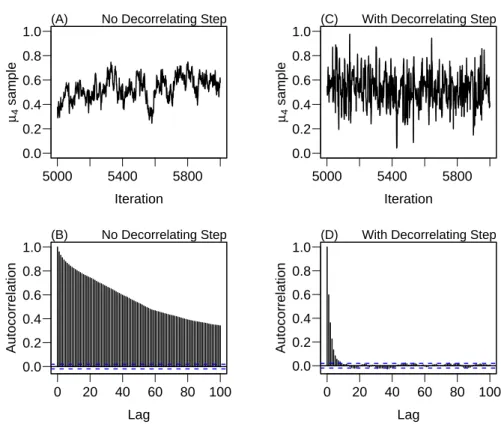
tic link function (dashed line). B: A hypothetical mapping from duration to true score for three participants. C: A hypothetical mapping from duration to probability correct for the same three participants. . . 19 2.3 Autocorrelation in MCMC Chains. A: Segment from the MCMC

chain for parameter µ

without a decorrelating step. B: autocorre-

lation function of parameter µ

. C & D: Segment from the MCMC

chain and autocorrelation with an additional decorrelating step. . 32

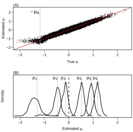
2.4 Results of simulation. A: Estimates of latent ability α as a function of true value. True latent abilities less than − µ

(vertical line) are from simulated participants whose performance is at chance for all of the items. B: Distribution of point estimates (posterior means) of µ

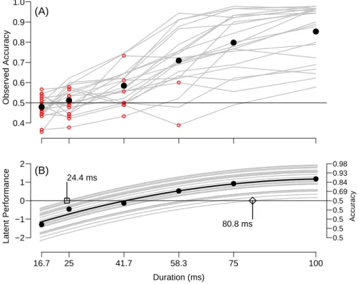
across replicates (smoothed histograms). The vertical lines represent the true values of each µ. . . 34 2.5 A: Mean and individual accuracy are denoted by dark points

and light lines, respectively. Open circles denote participant-by- duration combinations that are classified by the MAC model as below threshold. B: Points are estimates of duration condition ease µ

. Each line is a quadratic regression of true score on prime duration. The square and diamond symbols denote the smallest and largest thresholds estimated across the 22 participants. . . 39 2.6 Segments from the MCMC chains and autocorrelation functions

for selected parameters. . . 40 2.7 A: Observed accuracy as a function of predicted accuracy. Each

point denotes a participant-by-duration combination. Horizontal dashed lines represent the .025 and .975 quantiles of accuracy for a participant at chance. B: Standardized residuals from the MAC model. Light and dark lines denote participants for which the model is well-specified and misspecified, respectively. Horizontal dashed lines at -1.96 and 1.96 represent approximate 95% bounds on the residuals. . . 42 3.1 A. Autocorrelation for a select item effect (β

) from Gibbs Sam-

pling. B. Greatly reduced autocorrelation from the inclusion of

additional decorrelating Metropolis steps. The degree of autocor-

relation is typical for all participant and item parameters. . . 52

3.2 Simulation results. A-C: Two-dimensional kernel density esti- mates for estimated value as a function of true value for the param- eters α

, θ

, and x

= θ

(α

− β

), respectively. D-F: CDF coverage plots for model estimates of β

, β

, and β

. Dark points represent point estimates (posterior mean); light points on either side of each dark point represent corresponding 95% posterior credible intervals. The dark, solid vertical line represents the true value. . 56 3.3 Results of the described experiment and analyses. A: Accuracy

as function of stimulus duration for all 22 participants. Each line represents a participant. Participants marked ‘a’ and ‘b’ are the same participants shown in Figure 2.7B. B: 2P-MAC item diffi- culty (β) estimates as a function of duration. Error bars are 95%

credible intervals. Fitted regression line is best linear fit with weighted least squares. C: Ability estimates (α) as a function of discriminability estimates (θ) for all 22 participants. The square and diamond are Participants 1 and 2 from Panel A, respectively.

Right axis shows the threshold in ms corresponding to each abil- ity. D: Standardized residuals from the 2P-MAC analysis. The dark lines correspond to participants whose residuals were large and patterned in the 1P-MAC analysis (see Figure 2.7B). These residuals are greatly improved. . . 59 4.1 Proportion of participants who interrupted an experimenter as a

function of the type of sentences unscrambled in a previous task.

Figure adapted from Bargh, Chen, and Burrows (1996). . . 63

4.2 A: The structure of a trial in the number priming paradigm. The displayed prime is incongruent with the target. B: Predictions of four substantive priming theories. UnCON: priming reflects unconscious processes; CON: priming reflects conscious processes (Cheesman & Merikle, 1988); DUAL1: dual-process model of Snodgrass et al. (2004); DUAL2 dual process model based on Greenwald et al. (1996). The vertical line denotes the thresh- old on prime identification or categorization (Figure adapted from Snodgrass et al., 2004.) . . . 65 4.3 The regression method applied to data from a subliminal priming

experiment, from Draine and Greenwald (1998). Priming effect in a target categorization task is shown as a function of sensitivity in a prime detection task. The significant intercept is taken as evidence for subliminal priming. . . 68 4.4 The nonparametric regression of priming effect in a target catego-

rization task onto sensitivity in a prime categorization task. Ver- tical lines are standard errors of the mean. The nonmonotonicity is taken as evidence for a dual process model of Snodgrass et al.

Figure adapted from Snodgrass, Bernat, and Shevrin, (2004); data from Greenwald, Klinger, and Schuh (1995). . . 72 4.5 Results of Experiment 1. A: Mean priming effects in each prime

duration condition in the target categorization task. B: Mean

accuracies to categorize the prime in the prime categorization

task. C: Posterior probability of true baseline performance for

each participant-by-duration combination. Error bars in B and C

are standard errors of the mean. . . 78

4.6 MAC model analysis of Experiment 1. A: Bar plot showing the mean priming effect as a function of chance categorization status.

See text for an explanation of the Bayes Factor. B: Priming effect in mean RT as a function of latent ability x

. C and D: Same as A and B, but for the 10

RT percentile instead of the mean RT.

Error bars in A and C are 95% confidence intervals on the mean.

Open circles in B and D represent combinations categorized as below threshold. . . 80 4.7 MAC model analysis of Experiment 1, with standardized mean

RT. A: Bar plot showing the mean standardized priming effect as a function of chance categorization status. See text for an explanation of the Bayes Factor. Error bars are 95% confidence intervals on the mean. B: Priming effect in standardized mean RT as a function of latent ability x

. . . 81 4.8 Results of Experiment 2. A: Mean priming effects in each prime

duration condition in the target categorization task. B: Mean accuracies to categorize the prime in the prime categorization task. C: Posterior probability of true baseline performance for each participant-by-duration combination. Error bars in B and C are standard errors of the mean. . . 86 4.9 MAC model analysis of Experiment 2. A: Bar plot showing the

mean priming effect as a function of chance categorization status.

See text for an explanation of the Bayes Factor. B: Priming effect in mean RT as a function of latent ability x

. C and D: Same as A and B, but for the 10

RT percentile instead of the mean RT.

Error bars in A and C are 95% confidence intervals on the mean. . 87

4.10 MAC model analysis of Experiment 2, with standardized mean

RT. A: Bar plot showing the mean standardized priming effect

as a function of chance categorization status. See text for an

explanation of the Bayes Factor. Error bars are 95% confidence

intervals on the mean. B: Priming effect in standardized mean RT

as a function of latent ability x

. . . 88

Chapter 1

Thresholds in Psychology

The concept of a threshold has a long history in Psychology. Although Luce (1963) attributes the earliest mention of thresholds to the ancient Greeks, in modern times, the first comprehensive treatment of the threshold was Fechner’s (1860) Elements of Psychophysics. In this seminal work, Fechner describes how stimuli that are present, such as a very dim light or a low-intensity sound, can remain unperceived. In Fechner’s conception, a sensation may either rise to conscious awareness, or not. A threshold determines whether the sensation is intense enough to rise to awareness. In this way, Fecherian sensation is discrete;

either a sensation rises to a threshold or does not. One example of a model of sensation which makes use of discrete sensation is the high-threshold model (Blackwell, 1953). In this model, on each presentation of a stimulus there is a probability that it will rise above threshold and the participant will enter a state of detection. If the stimulus is not perceived, participants enter a non- detection state and guess that the stimulus was presented with some probability.

If no stimulus is presented, a participant will enter a non-detection state with probability 1.

In the mid-twentieth century, however, discrete models of perception were

challenged by continuous models. In continuous models, both stimulation and

the absence thereof gives rise to a range of graded perceptions. The most widely-

used continuous model of perception is the theory of signal detection (SDT; Green

& Swets, 1966). In SDT, there are no discrete detection and non-detection states.

When a stimulus is presented, it gives rise to a sensation strength that is a ran- dom variable, typically distributed as a normal. If no stimulus is presented, the sensation strength is a also a random variable, but one with a smaller mean than when a stimulus is presented. Observers are assumed to know these distributions well enough to be able to compute the likelihood that a given sensation strength comes from either the no-stimulus distribution or the stimulus distribution. Ob- servers place a criterion on the likelihood ratio, and they use this criterion to select a response.

This dichotomy between discrete and graded perception has characterized the field for over 40 years (see, for example, Luce, 1963a). In perception and memory, researchers have empirically differentiated these contrasting approaches through construction of receiver operating characteristic functions. The results seem clear—the data on whole better support continuous-perception models than discrete ones (Green & Swets, 1966; Swets, 1996, cf., Luce, 1963b). Based on this logic, Swets (1961) declared thresholds unnecessary, and the concept of a threshold has been discounted since. Thresholds today do not refer to levels of sensation needed to transition between discrete mental states; instead, they refer to levels of stimulus intensity that result in an select level of performance, say .75 or .707 (Taylor & Creelman, 1967). I use the term intensity throughout to generically to refer to any number of physical stimulus dimensions such as loud- ness, brightness, duration, etc. Perhaps the most poignant example of the lack of appeal of the concept of thresholds comes from the field of subliminal priming.

Subliminal priming refers to the phenomenon in which a stimulus that cannot

be detected can, nonetheless, influence subsequent behavior. Subliminal priming

seems to necessarily imply a notion of threshold. Even in this domain, however,

there is ambivalence. Greenwald, Klinger, and Schuh (1995), for example, write,

The term subliminal implies a theory of perceptual threshold, or li- men, that has has been largely abandoned as a consequence of the influence of signal detection theory (Green & Swets, 1966). A more theoretically neutral designation of the class of stimuli which this arti- cle is concerned is marginally perceptible. This article uses subliminal and marginally perceptible as interchangeable designations. (p. 22;

emphasis in original)

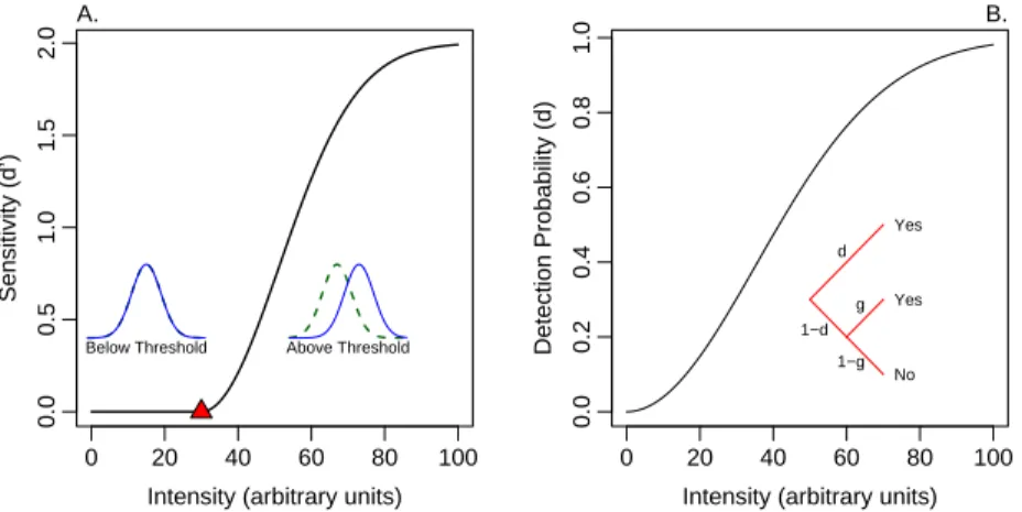
The concept of threshold has been discounted unnecessarily. The discounting arises because thresholds have been associated with discrete processing. This association, however, is not necessary; thresholds may be treated as logically independent from the nature of processing. Figure 1.1A shows an example of a threshold in a continuous processing model. The model is signal detection, and the main graph is a hypothetical relationship between stimulus intensity and sensitivity (the difference between the distribution means, d

). As shown, there is a threshold, denoted with a triangle at an intensity of 30. Stimuli with intensities below this threshold give rise to a range of percepts, but the distribution of these percepts is exactly the same as had there been no stimulation (see left insert). Stimuli more intense than the threshold result in distributions that differ as shown in the right insert. Figure 1.1B shows the opposite case—

discrete processing without a threshold. Responses are assumed to be governed by a high-threshold model (Blackwell, 1953) with d denoting the probability of detection. This probability is zero for a lack of stimulation. For any stimulus intensity value above zero, however, the probability of detection is above zero.

Even though processing is discrete, there is no positive intensity value for which the distribution of mental states is equivalent to a lack of stimulation.

The demonstration in Figure 1.1 motivates the following definition of thresh-

old. Let baseline refer to performance when there is a lack of stimulation. A

threshold is the maximum intensity for which true performance does not deviate

0 20 40 60 80 100

0.00.51.01.52.0

Intensity (arbitrary units)

Sensitivity (d’)

Above Threshold Below Threshold

A.

0 20 40 60 80 100

0.00.20.40.60.81.0

Intensity (arbitrary units)

Detection Probability (d)

B.

Yes

Yes

No d

1−d 1−g

g

Figure 1.1: A. An example of a threshold in a continuous-processing model. B.

An example of a lack of threshold in a discrete-processing model.

from baseline, or chance performance. This definition has the following proper- ties:

1. Thresholds are defined without recourse to underlying mental architecture, and, in particular, are compatible with graded perception.

2. The baseline level of performance associated with below-threshold stimu- lation is not arbitrary. For example, if participants observe either Stimulus A or Stimulus B on any trial and these two are presented equally often, then the baseline on accuracy is necessarily .5. This property contrasts with the arbitrariness of stipulating thresholds at a conventional level of performance, such as .75 or .707.

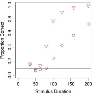
3. It is an open question whether thresholds exist. If thresholds do not exist, then the implication is that all stimulation, no matter how small, is reg- istered and affects the response on some nonzero proportion of the trials.

If thresholds do exist, then there is loss of information somewhere in pro-

cessing. The answer to whether thresholds exist probably depends on the

domain in question. Perhaps the clearest evidence for a threshold comes

from Loftus, Duncan, & Gehrig (1992) who manipulated the duration of briefly flashed and subsequently masked digits. Figure 1.2 shows their re- sults for two participants. They found that performance fell to baseline when the duration was less than a critical amount. Although this amount varied across participants, it was around 60 ms and was clearly above 0 ms. Busey and Loftus (1994), Shibuya and Bundesen (1988) and Townsend (1981) provide models that explicitly account for a threshold—stimuli that are not sufficiently intense have no effect on processing.

4. The concept of threshold is associated with specific performance measures.

Performance to any one stimulus may be assessed with multiple measures, each with its own threshold. For instance, in subliminal priming, perfor- mance to the prime is measured directly by accuracy and indirectly by its subsequent priming effect. The threshold on these two measures may differ.

The phenomenon of subliminal priming corresponds to a higher threshold for the accuracy measure than for the priming measure.

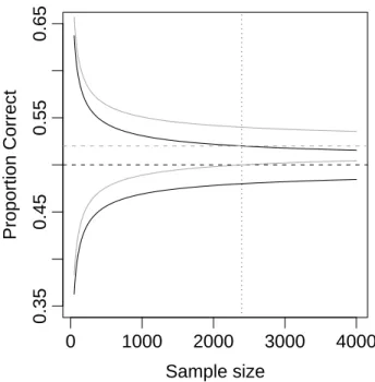
Although the above definition of threshold is advantageous from a theoret- ical perspective, it entails methodological complexities. The main problem is one of precision—it is difficult to determine if near baseline-levels of observed performance reflect baseline or slightly-above-baseline true levels. For instance, consider the case in which a participant identifies targets as either Stimulus A or Stimulus B and these two stimuli are presented equally often such that .5 is the appropriate at-chance baseline. Figure 1.3 shows the expected 95% CIs on accu- racy as a function of sample size for two levels of true accuracy: .5 and .52. The CIs from one level of accuracy exclude the other level after about 2,400 trials.

Restated, the power of excluding chance with a true accuracy of .52 with 2,400

trials is only 1/2. Unfortunately, it is rarely practical to run several thousand

trials per participant per condition.

Figure 1.2: Performance of two participants in a digit identification task with

a chance baseline of .10. Performance is around chance baseline for very brief

durations, then increases as duration is increased. Adapted from Loftus, Duncan,

and Gehrig (1992).

0 1000 2000 3000 4000

0.350.450.550.65

Sample size

Proportion Correct

Figure 1.3: Expected 95% CIs as a function of sample size for true accuracies of

.5 (dark lines) and .52. (light lines) . The vertical line at a sample size of 2395

shows the point at which the one level is outside the CI of the other.

In the psychological literature, various methods have been used to show that participants, or groups of participants are at baseline, each of which have serious drawbacks. I outline these methods briefly here and discuss the problems with their use.

• Confidence intervals: As discussed above, one way of testing that a specific participant is at baseline to see whether the 95% confidence in- terval around the observed performance score includes chance baseline.

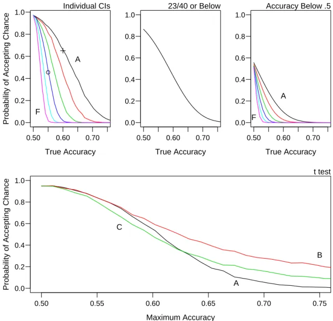
Figure 1.4, top-left panel, shows the probability of concluding baseline per- formance for various above-baseline levels of performance. The results are discouraging. The precision problems shown in Figure 1.3 cause very high error rates for reasonable sample sizes. For example, if the sample size is 50 trials (line A) and the participant has a true accuracy of .6, the proba- bility of concluding the stimulus is below-threshold is .65 (marked with an

“+”). Even at larger samples, this error rate remains high. For example, at 400 trials (third line from the left), true accuracy scores of .55 will be misdiagnosed as at baseline with a rate over 0.45 (marked with a “O”).

• Criteria on performance: Alternatively, researchers have claimed base- line performance by decreasing duration, in fine increments, until a thresh- old criterion was reached. For example, Dagenbach, Carr, and Wilhelm- sen (1989) decreased duration in increments of 5 ms until participants re- sponded correctly on no more than 23 out of 40 trials. Figure 1.4, top-center panel, shows why this approach is problematic. For Dagenbach et al.’s cri- terion, there is still a high probability of concluding baseline performance when true performance is substantially above chance. Another alternative is provided by Greenwald, Klinger, and Liu (1989), who selected partici- pants whose observed performance was below chance (i.e. accuracy was less than .5). The approach, however, is still susceptible to the same critique.

Figure 1.4, top-right panel, shows the probability of accepting baseline per-

0.50 0.60 0.70 0.0

0.2 0.4 0.6 0.8 1.0

True Accuracy

Probability of Accepting Chance

Individual CIs

F

A

0.50 0.60 0.70 0.0

0.2 0.4 0.6 0.8 1.0

True Accuracy 23/40 or Below

0.50 0.60 0.70 0.0

0.2 0.4 0.6 0.8 1.0

True Accuracy Accuracy Below .5

F

A

0.50 0.55 0.60 0.65 0.70 0.75

0.0 0.2 0.4 0.6 0.8 1.0

Maximum Accuracy

Probability of Accepting Chance

t test

A C

B

Figure 1.4: Probability of accepting chance performance as a function of true

accuracy. Top-left: 95% confidence intervals method. Lines A through F denote

sample sizes 50, 100, 200, 400, 800, and 1,600 respectively. Top-middle: Dagen-

bach et al.’s criterion of 23 of 40 correct responses.. Top-right: Greenwald et al.’s

selection of below-chance performance. Lines A through F denote sample sizes

50, 100, 200, 400, 800, and 1,600 respectively. Bottom: t test method. Lines A

through C represent the sample sizes from Murphy and Zajonc (1993), Exp. 1,

Dehaene et al. (1998), Tasks 1 and 2, respectively.

formance as a function of sample size. Once again, if true values are near .5, the method is susceptible to mistakenly concluding baseline performance.

• t test: Researchers have also made claims of baseline performance for groups of participants. Typically, the collection of individuals’ accuracy scores are submitted to a t test. The null hypothesis is that the true group average is at baseline and a failure to reject this null is taken as evidence that performance is at baseline for all participants. I highlight two influ- ential papers: Dehaene et al.’s (1998) investigation of the neural correlates of subliminal priming and Murphy and Zajonc’s (1993) demonstration of affective subliminal priming from emotive faces. Dehaene et al. asked six participants to discriminate numbers from blank fields (96 trials) and seven participants to discriminate numbers from letter strings (112 trials). For stimulus durations of 33 ms or less, they report that mean accuracies in both tasks were not significantly different from chance. Murphy and Za- jonc (1993) asked 32 participants to identify whether a briefly-presented face was happy or scowling on twelve trials. They too found that mean ac- curacy did not differ significantly from baseline. I assessed the probability of mistakenly accepting baseline performance with a t test through simula- tions. Each participant was assumed to have some degree of above-baseline performance. True accuracies were uniformly distributed between .5 and an upper bound. Figure 1.4, bottom, shows the probability of accepting the null as a function of the upper bound for the sample sizes in these ex- periments. Even for high values of this upper bound, there is a substantial probability of mistakenly concluding that performance for all participants was at baseline.

Figure 1.4 presents a troubling picture; it shows the difficulty of determin-

ing that stimuli are below threshold. Conventional null hypothesis tests

are ill-suited here because they do not offer appropriate safeguards from

mistakenly concluding baseline performance.

One way to gain the requisite precision is to pool data across participants.

To do so, item response theory (IRT; Lord & Novick, 1968) may be adapted to measure thresholds. Consider a two-choice identification experiment in which a participant decides if a target is Stimulus A or Stimulus B and the two are presented equally often. To find thresholds, the experimenter presents each of these stimuli at a number of intensities. The question is what is the maximum intensity such that performance is at the .5 baseline.

Consider the following one-parameter logistic (1PL) IRT model of perfor- mance in a psychophysical task. I refer to each intensity level of the stimulus as an item. Let y

, i = 1, . . . , I, j = 1, . . . , J , denote the number of correct responses in N

attempts for the ith participant observing the jth item:

y

indep.

∼ Binomial(N

, p

),

where p

is the true probability of correct response. In 1PL, p

= 1

2 + 1

2(1 + e

) , (1.1) where α

and β

denote the ability and difficulty of the ith participant and jth item, respectively. Participant abilities are zero-centered normal random variables with common variance. This model may be analyzed with a variety of methods (i.e., Andersen, 1973; Rasch, 1960; Swaminathan & Gifford, 1982).

One of the problems with 1PL is that it cannot measure a threshold. An

individual’s threshold in this case is the minimum value of β

necessary for p

=

.5. However, for all finite values of α

and β

, p

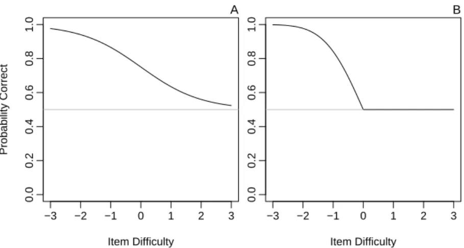
> .5. Figure 1.5A shows this

fact. The line is a person-response curve for the average person (α

= 0). As

difficulty increases, accuracy approaches the baseline but never attains it. This

incompatibility with thresholds holds for all links with support on ( −∞ , ∞ ) such

as the logit, probit, and t links.

−3 −2 −1 0 1 2 3

0.00.20.40.60.81.0

Item Difficulty

Probability Correct

A

−3 −2 −1 0 1 2 3

0.00.20.40.60.81.0

Item Difficulty

B

Figure 1.5: A. Person-response function for the average person in 1PL. B. The same for the MAC model.

Rouder, Morey, Speckman and Pratte (2007) proposed a truncated-probit link to model the transition in performance from baseline to above-baseline levels:

p(α, β ) =

Φ(α

− β

), α

> β

,

.5 β

≥ α

, (1.2)

where Φ is the CDF of the standard normal distribution. If the person’s ability is greater than the item’s difficulty, then performance is above baseline; conversely, if the item’s difficulty is greater than the person’s ability, then performance is at baseline. A person-response curve for an average person (α

= 0) is shown in Figure 1.5B. For all positive difficulties, performance is at baseline. For all negative difficulties, performance follows a probit. Because there is nonzero probability of baseline performance, Rouder et al. called this model Mass at Chance (MAC).

In the following chapters, I develop MAC models for determining whether

participants are at baseline. In Chapter 2, I develop a MAC model that allows

for multiple items, similar to a one-parameter logistic model. In Chapter 3, I

generalize the model to the two-parameter case. The final chapter illustrates the

use of the two-parameter model in two subliminal priming experiments.

Chapter 2

The One Parameter Mass at Chance Model

In previous work (Rouder et al., 2007), my colleagues and I proposed a Bayesian hierarchical model to select participants whose true prime identification perfor- mance is at chance. We termed this model the mass at chance model (MAC) to emphasize that a threshold is explicitly assumed and modeled.

Unfortunately, Rouder et al.’s MAC model has a pronounced limitation. Al-

though it controls the error rate in which above-chance true performance is

considered subliminal, it has a tendency to mistakenly classify true at-chance

performance as above chance. The reason for this is that paradigms with single

conditions provide very little information for the MAC model to use in classi-

fication. To provide for more efficient estimation of thresholds as well as more

efficient discrimination of at-baseline and above-baseline performance, in this

chapter I develop a one parameter MAC model. In the first section, I briefly

present the Rouder et al. MAC model and highlight its limitations. Following

that, I present the expanded paradigm and an expanded MAC model. I show

how this expanded model provides for highly accurate measurement of true per-

formance and, consequently, provides a methods for assessing priming theories

and estimating at-chance thresholds. Finally, I show how this model is similar

to the Rasch model (Lord & Novick, 1968) in Item Response Theory.

2.1 Rouder et al.’s MAC Model

The Rouder et al. MAC model was designed to account for performance in two-alternative forced-choice tasks including a threshold. At the first level of Rouder et al.’s MAC model, the number of correct prime identifications for the ith participant, i = 1, . . . , I, denoted y

, is

y

indep.

∼ Binomial(p

, N

). (2.1)

Parameter p

is the probability of a correct response and N

is the number of trials observed by the ith participant. For two-choice paradigms, primes are below threshold if p

= .5.

Each participant is assumed to have a true score, denoted x

. True probabil- ities (p

) are related to latent abilities:

p

=

.5, x

≤ 0,

Φ(x

), x

> 0, (2.2)

where Φ is the standard normal cumulative distribution function. The point x

= 0 serves as the threshold. If a participant has positive true score, then per- formance is above chance; conversely, if true score is negative, then performance is at chance. Negative true scores are interpretable: more stimulus energy is needed to bring the participant to threshold.

True scores are assumed to be random effects and distributed as normal in the population:

x

iid

∼ Normal(µ, σ

).

True scores depend on item factors. For example, the same participant will have higher true score to primes presented for 33 ms than to those presented for 22 ms.

This dependence is implemented by making µ dependent on stimulus intensity.

Rouder et al. (2007) developed MAC for a single parameter item parameter µ.

Priors are needed for µ and σ

. Based on extensive simulation, Rouder et al.

chose somewhat informative priors µ ∼ Normal(0,1) and σ ∼ Uniform(0, 1).

Participants are considered at-chance if much of the posterior distribution of x

is below zero. Therefore, the following posterior probability serves as a decision statistic:

ω

= Pr(x

< 0 | data). (2.3) The decision rule is

ω

≥ .95 → Conclude the participant is at chance

ω

< .95 → Conclude the participant is above chance (2.4) The main benefit of this approach is that it does not suffer from high rates of mistakenly claiming baseline performance, whereas the methods discussed in Chapter 1 do. In the MAC model, small sample sizes result in highly variable posterior estimates of x

. Consequently, there tends to be more mass above x

> 0. Lowering sample sizes makes it more difficult to claim that items are below-threshold rather than less difficult. Therefore, the MAC model provides an appropriate safeguard against high error rates in claiming baseline performance.

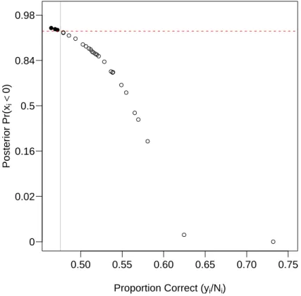
Although the MAC model provides a principled means for determining whether performance is at baseline, it has two major limitations. First, as mentioned pre- viously, the model does not select people as at chance often. Figure 2.1 shows ω

, the posterior probability that each participant is at chance, as a function of observed accuracy. The three closed circles represent participants selected as at chance. Although most of the 27 participants perform near chance, the model selects only three. The paradigm does not offer the model enough information to select more than three participants as at-chance, making it very difficult to use for researchers interested in below-threshold phenomena. Second, the MAC model is quite dependent to specification of the prior. In particular, the pos- terior of σ

was heavily influenced by the choice of prior

. This dependence is

1In typical paradigms, primes are designed to be below threshold. Consequently, much of the

Proportion Correct (y_i/N_i) Posterior Pr(xi<0)

0.50 0.55 0.60 0.65 0.70 0.75

0 0.02 0.16 0.5 0.84 0.98

Figure 2.1: Posterior probability that an individual participant is at chance as a function of observed accuracy. Participants whose posterior probability is above .95 (closed circles) are selected as at chance. (Figure adapted from Rouder et al., 2007)

undesirable.

These limitations may be mitigated by generalizing the model to multiple items. I extend the model for this case and find that: (1) the model allows for exceedingly accurate classification of performance as at-chance or above chance;

(2) the model is less dependent on the prior for variance.

mass of the distribution ofxi is below 0. Because participants at chance are indistinguishable from one another, estimation of the variance of the distribution of latent abilities can only be based on the prior and the performance of those participants above chance. When only a few participants are above chance, the prior has a large degree of influence.

2.2 The One Parameter MAC Model

It is straightforward to specify the extended MAC model for multiple items. We call the extended model 1P-MAC, according to Item Response Theory naming conventions, because of its similarity to the 1PL model described in Chapter 1.

Let y

, p

, and N

denote the number of correct responses, true probability of correct response, and number of trials, respectively, for the ith participant to the jth item:

y

∼ Binomial(p

, N

). (2.5) At the next level, it is assumed that for each participant-by-item combination, there is a true score, denoted x

. True scores determine probabilities on perfor- mance:

p

=

.5, x

≤ 0,

Φ(x

), x

> 0. (2.6) True scores reflects both the participant’s latent ability, denoted α

, and the ease of the item, denoted µ

in an additive manner:

x

= α

+ µ

. (2.7)

This additive model is borrowed from item response theory. Latent abilities are modeled as random effects:

α

∼ Normal(0, σ

).

The additivity assumption provides a convenient means of pooling informa-

tion about latent ability (α

) across items and about item ease (µ

) across partic-

ipants. This pooling allows for the possibility of estimating true score x

, even

when this true score is below threshold. The threshold for participant i is the

intensity for which the true score is x

= 0. The additivity assumption is made

with reference to the MAC link. It is impossible to assess whether additivity

holds without referencing a link. For example, if additivity holds for the MAC

link, it certainly will not for a logistic one, and vice-versa.

2.2.1 The MAC link function

In both Rouder et al.’s MAC model and the 1P-MAC model, true scores x

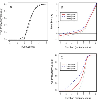
are mapped to probabilities using the half-probit link in Eqs. (2.2) and (2.6). This link function is shown as the solid line in Figure 2.2A. The MAC link differs from typical psychophysical functions. The former starts from a point and rises quickly without any inflection point. Psychophysical functions, however, tend to be characterized by a sigmoid-shaped function that has an inflection point.

Examples of the latter include the logit, probit, and cumulative distribution function of a Weibull with shapes around 2. The dotted line shows a logit link and the inflection point is clearly visible.

Given the success of previous inflected psychophysical functions in fitting ex- tant data, it would appear that the MAC link is unwarranted. This appearance, however, is deceiving. The MAC link is not a psychophysical function. It is a mapping from true scores into performance. True scores are latent rather than observed. Psychophysical functions, on the other hand, map physical charac- teristics of stimuli (e.g., duration) into performance. These characteristics are observed and are not latent. In the MAC model, the researcher estimates the relationship between stimulus characteristics and µ

, the latent ease of the stimu- lus. Because this relationship is estimated rather than assumed, the MAC model makes no commitments to the form of the psychophysical function.

Figure 2.2B-C provides a demonstration of how the MAC accounts for psy- chophysical functions with inflection points. Panel B shows hypothetical map- pings from duration to true scores for three participants. The additivity as- sumption in Eq. (2.7) implies that these mappings are parallel. Panel C shows the resulting mappings from duration to probability correct for the same three participants. The psychophysical functions in Panel C have inflection points.

If the MAC model is flexible enough to account for any psychophysical func-

tion, it is reasonable to wonder if the model is concordant with all data and,

−2 −1 0 1 2 3 0.5

0.6 0.7 0.8 0.9 1.0

True Score xij

True Probability Correct

A

2 3 4 5 6 7 8

−1 0 1 2 3 4 5

Duration (arbitary units)

True Score xij Participant 1

Participant 2 Participant 3

B

2 3 4 5 6 7 8

0.5 0.6 0.7 0.8 0.9 1.0

Duration (arbitary units)

True Probability Correct

Participant 1 Participant 2 Participant 3

C

Figure 2.2: A: The MAC half-probit link function (solid line) and a logistic link

function (dashed line). B: A hypothetical mapping from duration to true score

for three participants. C: A hypothetical mapping from duration to probability

correct for the same three participants.

thus, is vacuous. It is not. The model places constraints in two important ways.

First, the model describes how psychophysical links are distributed across the population. As seen in Figure 2.2C, the additivity of item ease and latent abil- ity results in specific relations between individual-level psychophysical functions.

For smooth convex mappings, such as those in Figure 2.2B, participants with smaller thresholds have smaller rates of gain in their predicted psychometric functions, as seen in Figure 2.2C. Second, the discontinuity in the first derivative of the MAC link ensures that there is an at-chance threshold in the psychophys- ical function. I discuss methods of assessing whether these constraints hold in data when analyzing the experiment.

Figure 2.2C shows that the MAC model, in general, does not predict par- allel psychometric functions across participants. This fact seems incongruous with themes in the field. Watson and Pelli (1983), for example, assume that psychometric functions across different conditions are parallel, that is, they are translation invariant. This assumption is common in many theoretical models including those of Green and Luce (1975), Roufs (1974), and Watson (1979); the empirical evidence for the invariance, however, is controversial (see Nachmias, 1981). The translation invariance considered is across conditions of similar stim- ulation; for example, across pulse trains of light flashes with varying numbers of pulses. Translation invariance across conditions, however, is not the same as translation invariance across participants. I do not know of any research focused on the latter. Nachmias’ (1981) results, however, may be used to empirically assess translation invariance across participants in a brightness detection task.

The estimates of the shapes of psychometric functions for some of conditions

varied widely across participants (Table 1, p. 220, Bipartite Field).

2.3 Prior Distributions

Analysis of the model is performed by Bayesian methods. Consequently, priors are needed for each µ

and σ

:

µ

iid

∼ Normal(µ

, σ

), (2.8) σ

∼ Inverse Gamma(a

, b

). (2.9) The inverse gamma distribution is commonly used as priors for variance in Bayesian analysis. The density function is

f (σ

| a

, b

) = (b

)

Γ(a

) (σ

)

exp

− b

σ

σ

, a

, b

> 0 (2.10) The parameters in the priors (µ

, σ

, a

, b

) are chosen before analysis. A non- informative Jeffreys prior may be placed on σ

by setting a

= b

= 0 (Jeffreys, 1961)

. I place a reasonable but informative prior on µ

by setting µ

= 0 and σ

= 1. To see why this prior is reasonable, consider an average participant with α

= 0. The Normal(0, 1) prior on µ

implies that the marginal prior on p

has half its mass at chance and is flat over (.5,1). If σ

is increased beyond 1.0, the marginal prior distribution on p

becomes increasingly bimodal with modes at .5 and 1. The prior parameters µ

= 0 and σ

= 1 were chosen as the most diffuse prior without bimodalities in the marginal prior on p for a participant with α

= 0. These choices convey information. To show that this information is not critical in analysis, I tried other values as high as σ

= 16. The effect is inconsequential.

2.4 Model Analysis

Although the model is straightforward to specify, analysis is complicated by the non-linearity in the MAC link. Closed-form expressions for the marginal

2With parametersa⁰=b⁰= 0, the prior onσ² becomes σ²∝(σ²)⁻¹. Although this prior is improper, the posterior will be proper ifI >2.

posterior distributions are not available. Instead, posterior quantities are esti- mated by Markov chain Monte Carlo techniques, specifically via Gibbs sampling (Gelfand & Smith, 1990). In this section, I provide the full conditional posterior distributions for parameters and provide efficient algorithms for sampling these distributions.

MCMC estimation of posterior distributions is greatly simplified by the data- augmentation method of Albert and Chib (1993; see Rouder & Lu, 2005, for a tutorial review). In the data-augmentation method, it is convenient to model the data as a collection of Bernoulli outcomes. Let y

be the outcome of the kth trial, k = 1, . . . , N

, for the ith participant to the j th item, where y

= 1 indicates a correct response and y

= 0 indicates an error. Accordingly,

P r(y

= 1) = Φ(x

∨ 0), where a ∨ b is max(a, b).

Let w

denote a normally-distributed latent random variable whose sign determines the correctness of the response:

y

=

0 w

≤ 0 1 w

> 0 The w

are distributed as

w

indep

∼ Normal(x

∨ 0, 1).

Then, P r(y

= 1) = P r(w

> 0). It is simpler to sample from the full condi- tional distributions of the parameters conditioned on the latent parameters w

than on data y

.

With the model specified, it is straightforward to define the joint posterior distribution. Let y be the collection of data, y =

D

h y

i

E

, and w be the collection of latent parameters, w =

D

h w

i

E

. The joint

posterior of all parameters is

[w, α, µ, σ

| y] ∝ Y

i

Y

j



 



 



Nij

Y

k=1

(yijk=0)

exp

− (w

− (α

+ µ

) ∨ 0)

2

I

×

Nij

Y

k=1

(yijk=1)

exp

− (w

− (α

+ µ

) ∨ 0)

2

I



 



 



× Y

i

(σ

)

exp

− α

2σ

× Y

j

exp

− (µ

− µ

)

2σ

× (σ

)

exp

− b

σ

. (2.11)

2.4.1 Full conditional distributions

I present the full conditional distributions of each of the parameters. Proofs are provided after each of the full conditional distributions. In this document, bold-face typeset is reserved for vectors, matrices, and multidimensional arrays.

Using this notation, y and w are the collection of all data y

and all latent variables w

; α and µ are the vectors of all α

and all µ

.

Fact 1. The full conditional posterior for σ

| α is σ

| α ∼ InverseGamma(a

+ I

2 , X

i

α

/2 + b

) (2.12) Proof of Fact 1: By inspection of (2.11), the full conditional posterior [σ

| α] is

[σ

| α] ∝ Y

i

(σ

)

exp

− α

2σ

× (σ

)

exp

− b

σ

.

Collecting like terms yields

[σ

| α] ∝ (σ

)

exp

−

1 2

P

i

α

+ b

σ

. (2.13) The right hand side of (2.13) is proportional to the density of an inverse gamma distribution with parameters a = a

+ I/2 and b = P

i

α

/2 + b

. 2

Fact 2. The full conditional posterior for w

| x

, y

w

| x

; (y

= 1) ∼ TN

(x

∨ 0, 1)

w

| x

; (y

= 0) ∼ TN

(x

∨ 0, 1). (2.14) where TN

(µ, σ

) denotes a normal distribution with parameters µ and σ

truncated below at l and above at u.

Proof of Fact 2: The full conditional distribution w

| y

, α , µ follows directly from the fact that the truncated normal is the distribution of a normal conditioned on a positive (or, alternatively, negative) outcome.

Fact 3. The full conditional posteriors of α

are independent for given µ, σ

, and w. It is convenient to define the following sets. Let A

= ( − µ

, ∞ ), A

= ( − µ

, − µ

), . . ., A

= ( −∞ , − µ

), where µ

< . . . < µ

are the order statistics of the µ

. Let

J

= { 1, . . . , J } J

=

j : µ

> µ

and define s

=

(

+ P

j∈Jℓ

N

0 ≤ ℓ < J

σ

ℓ = J (2.15)

m

=

( s

P

j∈Jℓ

P

k=1

w

− N

µ

0 ≤ ℓ < J

0 ℓ = J (2.16)

h

=

( P

j∈Jℓ

N

µ

− 2µ

P

k=1

w

0 ≤ ℓ < J

0 ℓ = J (2.17)

Then

[α

| µ, σ

, w] ∝

J

X

ℓ=0

exp

− 1 2

h

− (m

)

s

× exp

− (α

− m

)

2s

I

(2.18) Following Bayesian convention, [α

| µ, σ

, w] denotes the conditional den- sity of α

given µ, σ

, and w. The right-hand side of (2.18) is proportional to the density of a mixture of truncated normals. Set µ

= ∞ and µ

= −∞ . Let

q

= exp

− 1 2

h

− (m

)

s

p 2πs

×

Φ

− µ

− m

√ s

− Φ

− µ

− m

√ s

, (2.19) for ℓ = 0, . . . , J and let p

= q

/ P

ℓ=0

q

, ℓ = 0, . . . , J . Then the full conditional distribution [α

| µ, σ

, w] is the mixture of truncated normal distributions

α

| µ, σ

, w ∼

J

X

ℓ=0

p

TN

(m

, s

) (2.20)

Proof of Fact 3: Inspection of (2.11) reveals that the full conditional posterior of α

satisfies

[α

| µ, w, σ

] ∝ exp

− α

2σ

Y

j=1 Nij

Y

k=1

exp

− 1 2

(w

− α

− µ

)

I

+ w

I

.