The University of Manchester Research
Simulating the chemical kinetics of CO2-methane exchange in hydrate
DOI:
10.1016/j.jngse.2018.12.018
Document Version
Accepted author manuscript
Link to publication record in Manchester Research Explorer
Citation for published version (APA):
Gharasoo, M., Babaei, M., & Haeckel, M. (2018). Simulating the chemical kinetics of CO2-methane exchange in hydrate. Journal of Natural Gas Science and Engineering. https://doi.org/10.1016/j.jngse.2018.12.018
Published in:
Journal of Natural Gas Science and Engineering
Citing this paper
Please note that where the full-text provided on Manchester Research Explorer is the Author Accepted Manuscript or Proof version this may differ from the final Published version. If citing, it is advised that you check and use the publisher's definitive version.
General rights
Copyright and moral rights for the publications made accessible in the Research Explorer are retained by the authors and/or other copyright owners and it is a condition of accessing publications that users recognise and abide by the legal requirements associated with these rights.
Takedown policy
If you believe that this document breaches copyright please refer to the University of Manchester’s Takedown Procedures [http://man.ac.uk/04Y6Bo] or contact uml.scholarlycommunications@manchester.ac.uk providing relevant details, so we can investigate your claim.
Simulating the chemical kinetics of CO
2-methane exchange in hydrate
Mehdi Gharasoo1,2,*, Masoud Babaei3, and Matthias Haeckel4
1Technical University of Munich, Chair of Analytical Chemistry and Water Chemistry, Marchioninistr. 17, 81377 Munich, Germany
2Helmholtz Zentrum M¨unchen, Institute of Groundwater Ecology, Ingolst¨adter Landstr.
1, 85764 Neuherberg, Germany
3University of Manchester, School of Chemical Engineering and Analytical Science, Manchester, M13 9PL, UK
4GEOMAR - Helmholtz Centre for Ocean Research, Department of Marine Geosystems, Wischhofstraße 1-3, 24148 Kiel, Germany
*Corresponding author. Tel.: +49 89 3187 3498; E-mail:
mehdi.gharasoo@helmholtz-muenchen.de
October 27, 2018
Abstract
1
Carbon dioxide exchange with methane in the clathrate structure has been shown ben-
2
eficial in laboratory experiments and has been suggested as a field-scale technique for pro-
3
duction of natural gas from gas-hydrate bearing sediments. Furthermore, the method is
4
environmentally attractive due to the formation of CO2-hydrate in the sediments, leading
5
to the geosequestration of carbon dioxide. However, the knowledge is still limited on the
6
impact of small-scale heterogeneities on hydrate dissociation kinetics. In the present study,
7
we developed a model for simulating laboratory experiments of carbon dioxide injection into
8
a pressure vessel containing a mixture of gas hydrate and quartz sand. Four experiments
9
at different temperature and pressure conditions were modeled. The model assumes that
10
the contents are ideally mixed and aims to estimate the effective dissociation rate of gas
11
hydrate by matching the model results with the experimental observations. Simulation re-
12
sults indicate that with a marginal offset the model was able to simulate different hydrate
13
dissociation experiments, in particular, those that are performed at high pressures and low
14
temperatures. At low pressures and high temperatures large discrepancies were noticed be-
15
tween the model results and the experimental observations. The mismatches were attributed
16
to the development of extremely heterogeneous flow patterns at pore-scale, where field-scale
17
models usually assume the characteristics to be uniform. Through this modeling study we
18
estimated the irreversible dissociation rate of methane- and CO2-hydrate as 0.02 and 0.03
19
mol.m-3s-1, respectively.
20
Keywords: CO2 injection; CO2-methane exchange; Gas-hydrate recovery; Small-scale
21
heterogeneities; Kinetic modeling
22
1 Introduction
23
Gas-hydrates are solid clathrate compounds that are thermodynamically stable at low temper-
24
atures and high pressures. Such conditions naturally exist below permafrost and in deep ocean
25
sediments in which immense amount of methane is estimated to be stored as gas-hydrate de-
26
posits (Archer et al., 2009; Burwicz et al., 2011). The global amount of gas-hydrate deposits
27
have been reported between 1015and 1018standard cubic meters (Pi¯nero et al.,2013;Wallmann
28
et al., 2012), or about 15 Tera tonnes of oil equivalent (Makogon, 2010) which is adequate for
29
maintaining the supply of energy for centuries. Although the range of estimates is wide, it is
30
agreed that the available amount of gas-hydrate deposits is huge and thus worth of the atten-
31
tion as an alternative source of energy. Development of strategies for extraction of methane
32
from gas-hydrate reservoirs has recently become an economically attractive option given the
33
environmental desirability of natural gas as a fuel in comparison to other fossil fuels.
34
Methods of producing natural gas from gas-hydrates are mainly based on disturbing the ther-
35
modynamic stability of gas-hydrate in the reservoir leading to dissociation of the gas-hydrate
36
and release of the methane. The methods include (i) thermal stimulation by increasing the tem-
37
perature in the reservoir (e.g.,Fitzgerald and Castaldi,2013), (ii) depressurization (e.g.,Ahmadi
38
et al.,2007), (iii) hydrate conversion by substituting gas molecules inside the gas-hydrate crystals
39
with another similar gas (e.g.,Kvamme et al.,2007,2016;Ohgaki et al.,1996), and (iv) injection
40
of thermodynamic inhibitors (e.g., amino acids, salts, alcohols or non-ionic surfactants) (Erfani
41
et al.,2017;Masoudi and Tohidi, 2005) for altering phase equilibrium conditions. Amongst all
42
these methods, the conversion of methane-hydrate to CO2-hydrate by injection of CO2 has par-
43
ticularly attracted attentions since carbon dioxide is shown to be able to displace methane in the
44
hydrate lattice provided that both gases form a similar hydrate structure (type SI) (Kvamme
45
et al.,2016;Ohgaki et al.,1996;Voronov et al.,2014). The replacement of guest molecules can
46
happen either directly without dissociation of the hydrate structure or indirectly through con-
47
secutive dissociation of methane-hydrate and formation of CO2-hydrate. Goel (2006) discussed
48
that the introduction of carbon dioxide to the reservoir and its conversion to hydrate is alone suf-
49
ficient to thermodynamically maintain the dissociation of methane-hydrate. The CO2-methane
50
exchange, regardless of its exchange mechanism, is particularly interesting for its capacity to
51
sequester carbon dioxide in favor of reducing greenhouse gas emissions (see e.g., Dashti et al.,
52
2015;Kvamme et al.,2007). The method also has a couple of other side benefits such as main-
53
taining the mechanical stability of the reservoir preventing sea-floor landslides in field operations
54
(Sultan et al.,2004), and the potential for thermal stimulation through the injection of super-
55
critical carbon dioxide (Deusner et al., 2012; Ebinuma, 1993). The feasibility of CO2-methane
56
exchange as a technology to produce natural gas from gas-hydrate zones has already been pro-
57
posed and investigated (e.g., Yonkofski et al., 2016). Many other studies, e.g., Kvamme et al.
58
(2016);Deusner et al.(2012);Ota et al.(2005), analyzed the outcome of CO2-methane exchange
59
at laboratory scale using apparatuses in which carbon dioxide (either gas or liquid) is injected
60
into a vessel containing methane-hydrate. A substantial number of studies have used numerical
61
models to evaluate the conventional methods of production from gas-hydrate reservoirs (e.g.,
62
Moridis and Reagan,2011a,b;Vafaei et al.,2014). However, numerical studies on CO2-methane
63
exchange are few and are mostly limited to the field-scale. For example, White et al. (2011)
64
modeled the injection of carbon dioxide into a depressurized gas-hydrate reservoir and stated
65
that the low injection pressures of carbon dioxide can enhance the methane recovery from class
66
1 hydrate.
67
Although significant research efforts have been dedicated to the development of efficient ex-
68
perimental procedures and reliable models[they may ask for references], the complex reaction
69
kinetics of CO2-methane exchange at the scales of pore to core has not yet been addressed in
70
detail or experimentally constrained under the controlled conditions. Most of current modeling
71
approaches [e.g. ???] simplify the reaction kinetics (usually employ a simple first-order kinet-
72
ics) and neglect the small-scale heterogeneities at the scale of their computational grid (where
73
the transport properties are averaged and considered constant).
74
In contrast to the existing modeling studies that mostly concentrated on complexity of
75
fluid dynamics at large scales (and simplified the reaction kinetics due to uprising numerical
76
instabilities), the present model focuses on complexity of the reaction kinetics and simplifies
77
the fluid flow mechanisms. To this end, the approach provides a measure to gauge the lone
78
importance of kinetics at small scales where heterogeneities are typically ignored. The overall
79
aim is thus to use the numerical simulations to unravel the extent of influence that typical
80
assumptions of simplifying reaction kinetics and ignoring pore-scale heterogeneities have on the
81
accuracy of estimations at small scales, and to illustrate the contributions of error to field-scale
82
modeling calculations. Are you sure about the word uprising above? Furthermore, the
83
literature and approximates/testifies the effective rate parameter values for the experimental
85
results of Deusner et al. (2012). For this purpose, a rigorous optimization technique (Babaei
86
and Pan,2016) was applied to fit the model to the experimental results.
87
The paper is structured as follows: first we describe the model structure and its underlying
88
assumptions. Then, the governing equations of hydrate dissociation/formation kinetics, mass
89
and energy balance are introduced. Next, we describe the optimization formulation to calibrate
90
the system kinetics using existing experimental data fromDeusner et al.(2012). Finally, results
91
are presented and discussed.
92
2 Experimental Setup
93
Deusner et al. (2012) examined methane production from hydrates by injection of supercritical
94
carbon dioxide into a pressure vessel containing a water-saturated mixture of methane-hydrate
95
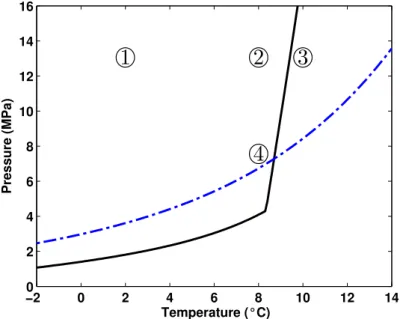
and quartz sand. The experiments were performed at four different pressure-temperature con-
96
ditions that are typical for naturally formed gas-hydrate reservoirs (Fig. 1).
97
The sediment samples were prepared at -20°C from a homogeneous mixture of quartz sand
98
(grain size of 0.1-0.6 mm) and fine ice particles (grain size fraction of 0.3-1 mm) produced from
99
deionized water. Experiments were carried out in a custom-made high pressure stainless steel
100
apparatus. Supercritical CO2 was injected with a piston pump from an inlet at the bottom of
101
the sample vessel and was heated to 95 °C inside temperature controlled conditioning chamber
102
prior to the injection. Pressure, salinity and temperature were continuously monitored and
103
recorded at the inlet and outlet. To achieve a constant rate of injection, pressure was adjusted
104
with a back-pressure regulator valve in line with a fine-regulating valve for the compensation of
105
pressure spikes. At the beginning of every CO2 injection interval, the sediment-hydrate sample
106
was continuously percolated with saltwater at a flow rate of 1.0 ml.min-1. The water pre-wash
107
was performed to ensure that the sample body was permeable and homogeneously pressurized.
108
CO2 was injected stepwise following a sequential injection strategy and completed after a four
109
to six injection rounds with CO2 supply rates of 2.5 to 5 ml.min-1. The waiting time between
110
the injection intervals are referred to as equilibration intervals during which no effluent fluid was
111
produced and the system was left to reach thermodynamic equilibrium. During the equilibration
112
intervals, the system pressure was maintained by the injection of a small amount of CO2in order
113
to compensate the volume changes due to CO2 cooling and phase changes. The CO2 injection
114
intervals and the waiting time between them were different for each experiment.
115
Experiments were performed at three ambient temperatures (2, 8 and 10 °C). The temper-
116
ature was regulated at the exterior surface of the vessel with a thermostat system and kept
117
constant through the entire experiment. At the start of experiment, the vessel included only
118
three components: methane, water and quartz sand. Methane and water initially existed as
119
methane-hydrate. The quartz sand was assumed nonreactive and regarded as an inert solid
120
phase. During injection intervals, the introduction of hot CO2 altered the system thermody-
121
namics and new additional components such as liquid CO2 and gaseous methane were identified
122
(Fig. 2). CO2-hydrate formation was also viable depending on system p/T conditions during
123
equilibration. It was impossible to exactly determine the final composition of gas-hydrate at the
124
end of the experiments. There is, however, a high possibility that a mixed CO2-CH4-hydrate
125
was formed in the vessel. Nevertheless, the mixed composition of gas-hydrates could not influ-
126
ence the mass balance calculations which were done based on component inventories and by the
127
volume balancing of inputs and outputs. See Deusner et al.(2012) for further details about the
128
experiments and the assembly of apparatus.
129
3 Materials and Methods
130
The model describes the experimental pressure vessel as an isobaric perfectly mixed reactor. In
131
this modeling approach, the system was considered homogeneous and the chemical components
132
inside it were assumed ideally mixed.
133
In the model, superheated liquid CO2 entered from the inlet during the injection periods
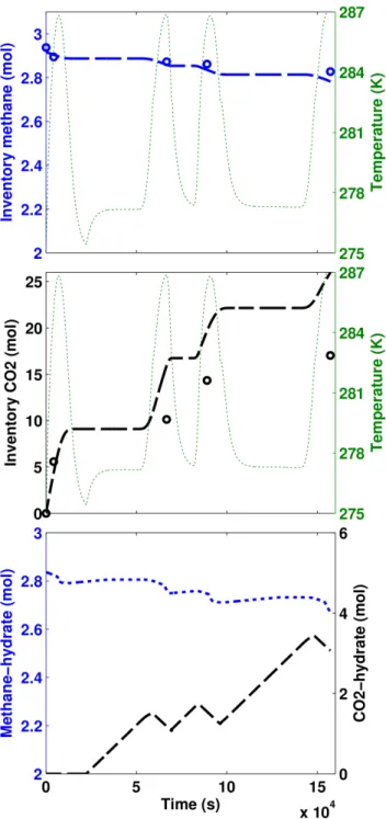
134
and dissociates the methane-hydrate in place. Then the system is left to reach the equilibrium
135
and this cycle repeats for several times according to the experimental procedure. Given that
136
the vessel pressure was kept constant during the entire experiment, the mobile substances (e.g.,
137
water, CO2and methane) were allowed to discharge from the outlet during the injection intervals
138
only. The outlet composition was assumed identical to the composition of the substances inside
139
the reactor, which itself is a function of residence time and the reaction kinetics. Depending on
140
the p/T conditions in the vessel, CO2- or methane-hydrate could form during the equilibrium
141
intervals. The terms CO2-hydrate and methane-hydrate in this modeling study represent the
142
components CO2 and methane incorporated in the gas-hydrate phase. The thermodynamics of
143
3.1 Governing equations
145
3.1.1 Mass balance
146
System mass balance follows the equation (COMSOL 4.3,2013),
147
d(cjVr)
dt =vjci,j−vjcj+rjVr (1) whereVris the volume of reactor, cj is the concentration of substancej(Water, CO2, methane,
148
etc.) in the system,ci,j is the concentration of substance jat the inlet,vj is the rate of influent
149
stream to the system (equal to effluent) andrj is the increase/decay rate of substancejaccording
150
to the reactions.
151
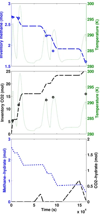
3.1.2 Energy balance
152
The solution of energy balance gives (COMSOL 4.3,2013):
153
VrX
j
cjCp,jdT
dt =Qr+Qw+X
j
vjci,j(hi,j−hj) (2)
where hj is the enthalpy of substance j, Cp,j the heat capacity of substancej,Qw the amount
154
of energy lost or gained through the reactor walls, and Qr the energy consumed or released by
155
reactions,
156
Qr=VrX
k
Hkrk (3)
withHk as the enthalpy of reactionk. Qw is calculated analytically for the cylindrical shape of
157
reactor:
158
Qw = 2πLλm(Ts−T) (4)
where T is the system temperature, L the length of vessel, and Ts is the temperature at the
159
inner surface of reactor wall calculated by
160
Ts= λmT+λwTw
λm+λw (5)
with λm andλw calculated as,
161
λm= κm
ln(rs/rin), λw= κw
ln(ro/rs) (6)
wherers is the reactor inner radius,rin is the radius of inlet,rois the reactor outer radius,κw is
162
the thermal conductivity of the wall material and κm is the overall thermal conductivity of the
163
system calculated byκm=P
sjκj whereκj is the thermal conductivity andsj is the saturation
164
of substances inside the vessel calculated bysj =cjφMj/ρj. φis the porosity of vessel,Mj is the
165
molecular weight and ρj is the density of substance j. The enthalpy of substances at different
166
system temperatures are calculated as,
167
hj(T) = Z T
0
Cp,jdT +hj(0) (7)
wherehj(0) is the enthalpy of substancejat a reference temperature and pressure. hj(0) values
168
at 293K and 13MPa for methane, CO2 and water were calculated 12.25, 10.5 and 1.72 kJmol-1
169
respectively (NIST Chemistry WebBook, Linstrom and Mallard,2013). Cp,j was assumed con-
170
stant for the p/T conditions of experiments.
171
3.1.3 Reactions
172
The solution of mass and energy balance considers the following reactions inside the reactor.
173
Depending on the p/T conditions, hydrate dissolution and formation occur inside the hydrate
174
stability region and hydrate dissociation occurs outside the hydrate stability region (see Fig. 1).
175
The following pair of reversible reactions were considered under the stability conditions:
176
CH4.6H2O ↔CH4(aqueous)+ 6H2O (8a)
CO2.6H2O ↔CO2(aqueous)+ 6H2O (8b)
Reactions 8a-8b account for hydrate dissolution while thermodynamically stable, but under-
177
saturated with respect to the gas in the solution (water). Hydrate precipitation (formation)
178
occurs at over-saturated conditions. A set of irreversible reactions were considered for p/T
179
conditions at which hydrates are thermodynamically unstable,
180
CH4.6H2O →CH4(aqueous)+ 6H2O (9a)
CO2.6H2O →CO2(aqueous)+ 6H2O (9b)
Reactions9aand9baccount for disintegration of hydrate when it is not stable. Since during the
181
experiments the pressure of the system was kept constant, the stability of hydrates in model was
182
determined only by the system temperature. The hydrate instability occurred when the system
183
temperature exceeded the hydrate stability temperature Tc. For the experiments at 13MPa,
184
the stability temperatures for CH4-/CO2-hydrate were measured from stability curves (Fig. 1)
185
at 13.7/9.5 °C, respectively. These values were lower for the experiment at 8MPa and were
186
determined to be 8.95 and 8.9 °C for CH4- and CO2- hydrate, respectively.
187
According toHaeckel et al.(2004) the rate of hydrate dissolution/formationrj was calculated
188
by,
189
rj =
(krev,j(ccte,j−cHydratej) if T < Tc, (10a)
kirr,j if T > Tc. (10b)
Under hydrate stability condition, krev,j is defined based on the Arrhenius formula,
190
krev,j =Aje−
∆Ej
RcT (11)
where T is the system temperature, Rc is the universal gas constant, and for hydrate j, Aj
191
denotes the frequency factor and ∆Ej the activation energy (Table1). Aj is typically expressed
192
in [mol.m-2.s-1.Pa-1] and to convert its unit to [s-1] the following equation is used (Kim et al.,
193
1987):
194
Aj[s−1] = 6Psys Ψρjdj
Aj[molm−2s−1P a−1] (12)
wheredj is the average diameter of hydrate particles,Psysis the system pressure,ρjis the hydrate
195
molar density, and Ψ is the particles geometry term (Ψ = 1 for spherical particles). According
196
toHaeckel et al.(2004), Eq. (10) assumes hydrate dissolution or formation to be proportional to
197
the saturation of methane in pore water with respect to its equilibrium concentration (ccte). At
198
hydrate instability conditions (at system temperatures above the stability temperature) kirr,j
199
was assumed constant and treated as an adjustable parameter.
200
The exchange rate of methane and CO2 from pure phase to the water phase and vise-versa
201
is defined by the following reversible reactions,
202
CO2(liquid)↔CO2(aqueous) (13a)
CH4(gas)↔CH4(aqueous) (13b)
where the exchange rates follow the same mechanism as of Eq. (10) without the temperature
203
dependencies, and similar to Noyes et al.(1996),
204
rj =ks,j(ccte,j−cj).
The exchange rate constants ks,j are estimated by the fitting procedure. The values of ccte
205
for aqueous CO2 and methane, and both CO2- and CH4-hydrates at experimental temperatures,
206
pressures and salinity are calculated according to Henry’s law and listed in Table1.
207
3.2 Optimization technique
208
Interior-reflective Newton methods (Coleman and Li, 1996; Gharasoo et al., 2017) which are
209
often employed in solving optimization problems have difficulties in minimizing this model due
210
to high nonlinearity and discontinuity of the objective function. We thus used a hybrid response
211
surface surrogate-based method which also reduces the computation costs of the optimization
212
process. The details of the algorithm is presented inBabaei and Pan (2016) where the authors
213
showed that the surrogate model that most consistently and robustly results in a computationally
214
efficient optimization operation is the Radial Basis Function (RBF).
215
We first define normalized root-mean-square derivations (NRMSD) for inventory CH4 and
216
CO2 as functions of four unknown parameters kirr,M GH ,kirr,CGH ,ks,CH4 , and ks,CO2:
217
NRMSDCO2 = q
E((CO2inv.)−(CO2inv.exp))2
max(CO2inv.exp)−min(CO2inv.exp) (14a) NRMSDCH4 =
q
E((CH4inv.)−(CH4inv.exp))2
max(CH4inv.exp)−min(CH4inv.exp) (14b) where E is the mean square error function, CO2inv., CO2inv.exp, CH4inv., and CH4inv.exp
218
are respectively the inventory CO2 calculated from the numerical model, inventory CO2 calcu-
219
lated from experiment, inventory CH4 calculated from the numerical model and inventory CH4
220
calculated from experiment. The objective function to be minimized is written as
221
f(kirr,M GH, kirr,CGH, ks,CH4, ks,CO2) =
4
X
i=1
(NRMSDCO2 + NRMSDCH4) (15) where subscript i refers to experiment 1 to 4. Next using the flowchart of Babaei and Pan
222
(2016)[Fig.4], f(kirr,M GH, kirr,CGH, ks,CH4 is treated as F(ucandidtae). Instead f using any en-
223
semble surrogates, we use RBF to generate surrogates of the actual solver. The number of
224
function evaluations for Latin hypercube sampling (NLHS) and the total number of function
225
evaluations that calls the actual solver (Neval) are set equal to 40 and 100. Babaei and Pan
226
(2016) used NLHS= 2n+ 2 (where nis the number of state variables, for our case n= 4), and
227
Neval = 2.5NLHS to successfully optimize a complex problem with four variables. Therefore, in
228
this study, NLHS = 20 and Neval = 50 are sufficient for optimization of objective function for
229
four parameters (u) using RBF. Furthermore, formulation of the objective function as above
230
considers all experiments conducted in this study and both measured inventory compounds.
231
The inventory CO2and methane basically include all forms of the compound in the vessel (pure
232
(liquid or gaseous), aqueous, and hydrate), and can simply be calculated from the model as
233
follows:
234
CO2inv. =CO2(liquid)+CO2(aqueous)+CO2(hydrate) (16a) CH4inv. =CH4(gas)+CH4(aqueous)+CH4(hydrate) (16b)
Note that methane cannot exist in liquid form in our experimental p/T conditions.
235
3.3 Model implementation
236
The model was implemented in COMSOL Multiphysics® using itsReaction Engineering Mod-
237
ule. Two modeling setups, a batch and a reactor, were employed and coupled together. The
238
inert components (gas-hydrates and sand) were simulated by the batch model and the mobile
239
substances (water, CO2 and methane) by the reactor model. The two modeling setups were
240
linked together to ensure a correct mass and energy balance for the entire system. The chemical
241
parameter values for hydrates and other components were taken from the literature or NIST
242
Chemistry WebBook (Linstrom and Mallard,2013), listed in Table1.
243
To maintain the model numerical stability, any sudden change of the boundary conditions
244
as well as shift of hydrate thermodynamics (from stable to instable and vice versa) at stability
245
temperatures must be treated continuously. To that end, the CO2 injection intervals in model
246
were smoothed using a second derivative smoothing technique (COMSOL 4.3,2013;Vermolen
247
et al., 2009). A rigorous method was also applied for the definition of the local reaction rates
248
(Section 3.1.3) to ensure a smooth transition of hydrate reaction rates from stable towards
249
unstable conditions.
250
The COMSOL code is converted to functionf(kirr,M GH, kirr,CGH, ks,CH4with state variables
251
as inputs and via COMSOL-MATLAB LiveLinkTM, optimization is carried out in MATLAB
252
treating COMSOL as a black-box. We use MATSuMoTo toolbox in MATLAB to call RBF to
253
construct surrogate model of COMSOL function (M¨uller and Pich´e, 2011; M¨uller, 2014) and
254
speed up the optimization process.
255
3.4 Simulated scenarios
256
Four scenarios were simulated at the following pressure-temperature conditions where the ex-
257
perimental data are available (Deusner et al.,2012):
258
experiment 1: 13 MPa/2 °C
259
experiment 2: 13 MPa/8 °C
260
experiment 3: 13 MPa/10 °C
261
experiment 4: 8 MPa/8 °C
262
The phase diagram in Fig. 1 illustrates the experimental conditions with respect to the
263
thermodynamic stability regimes of CH4- and CO2-hydrate. The experiments were performed
264
in a pressure vessel of 38 cm length, 8 cm cross section diameter, 18 mm casing thickness, with
265
inlet (and outlet) of 13 mm diameter (Deusner et al.,2012).
266
The simulation developed to calibrate four experiments described above models a reactor
267
with nearly two liters volume in which 95 CO2was injected during multiple intervals separated
268
with periods of equilibrium.
269
4 Results and Discussion
270
4.1 Modeling results
271
In the present study, the major modeling results of interest are the temporal changes of (1) the
272
reactor’s average temperature, (2) the overall methane and CO2 inventory, (3) the amount of
273
methane- and CO2- hydrate, and (4) the overall system thermal conductivity (Figs. 3 to 6).
274
In the experiments, only the total amount of inventory methane and CO2 (including all pure,
275
dissolved or hydrate phases) was calculated using outlet and inlet volume balancing. Therefore,
276
the primary aim was to obtain a proper fit first with the methane inventory data and then
277
with the CO2 inventory data, and then use the model to predict the fluctuations of temperature
278
and gas-hydrate in the system. Since it was very difficult to directly record temperature values
279
or determine the amount of gas-hydrates inside the pressure vessel, the use of model (after
280
constraining the unknown parameters) helped to calculate these quantities that otherwise were
281
unobtainable by means of laboratory equipments.
282
It is easy to approximately locate the start and the duration of injection intervals in Figs.3
283
to 6 where abrupt temperature changes occurs. The system’s highest temperatures are gen-
284
erally observed during the injection times when the average temperature of the system raised
285
due to the entry of 95°C CO2. In all experiments, the majority of methane-hydrate dissociation
286
occurred during the injection intervals when the system’s temperature increased above the hy-
287
drate stability temperature. Hence, the quicker the system reached or the longer it stayed at
288
hydrate instability conditions, a higher amount of hydrate dissociation was obtained. In con-
289
trast, the accumulation or precipitation of hydrate mainly occurred during equilibration periods
290
after the system lost heat to the surroundings. Further details and distinguishing features for
291
every modeling scenario are separately addressed in the following sections.
292
4.1.1 First scenario: 13 MPa/2 °C
293
The first experiment was performed at the lowest temperature leading to the lowest amount of
294
methane-hydrate dissociation and the highest amount of CO2 accumulation. The experiment
295
time was about 44 hours in which the CO2was injected in four separate intervals. The maximum
296
temperature reached only 285 K and was mainly achieved at the peak of injection intervals. Due
297
to very low ambient temperature and high vessel pressure, the system hydrates were exposed to
298
instability conditions only for a very short time. Most of the CO2 was, therefore, speculated to
299
deposit in the vessel as CO2-hydrate with excess pore water. The modeling results also confirmed
300
the accumulation of CO2-hydrate in the system. The qualitative model reproduction of the
301
experiment data of the CO2inventory supports this hypothesis and also suggests a homogeneous
302
retention of the injected CO2 in the vessel (Fig. 3).
303
The long equilibration periods between the injection intervals allowed CO2 to slowly form
304
CO2-hydrate and increased its retention yield. The model predicted the formation of nearly
305
3 mol CO2-hydrate inside the vessel while the methane-hydrate dissociation was predicted to
306
be less than 0.1 mol. A substantial formation of CO2-hydrate with the excess pore water was
307
confirmed and was speculated as the main reason preventing rapid growth of preferential flow
308
paths in this scenario.
309
4.1.2 Second scenario: 13 MPa/8 °C
310
In comparison to the first experiment, the second experiment was done at a higher ambient
311
temperature and therefore a significantly higher amount of methane-hydrate dissociation was
312
observed (Fig. 4). While the length of experiment was marginally longer than the first experi-
313
ment (about 45.5 hours), a higher amount of CO2 was injected through five intervals (25% more
314
CO2 was injected in comparison to the first experiment). The amount of heat transfered to the
315
vessel was therefore higher but this was not the only feature contributing to a higher amount
316
of methane-hydrate dissociation. In this scenario, the system was exposed to the hydrate insta-
317
bility conditions for a longer time thereby increasing the methane yield. Evidently, the small
318
temperature difference between the experiment’s initial condition and the hydrates instability
319
of a larger amount of methane-hydrate (the second highest amongst all experiments). The CO2
321
inventory was overestimated by the model. This suggests that the injected CO2 was possibly
322
conveyed through preferential flow paths that were created due to methane-hydrate dissocia-
323
tion. Other factors such as consecutive injections, and a short equilibration time between the
324
injection intervals, could also have enhanced the progression of the preferential flow paths in
325
this experiment.
326
4.1.3 Third scenario: 13 MPa/10 °C
327
The third experiment was done at the highest ambient temperature during which the CO2-
328
hydrate was subjected to instability conditions for the entire duration of the experiment and
329
therefore never formed. The modeled CO2 inventory curves deviated even more from the ex-
330
perimental data indicating once again the development of preferential flow paths prohibiting a
331
spread of CO2 into the reactor volume. Comparing the results with the previous scenarios, it
332
is speculated that the development of preferential flow paths are even stronger and that the
333
formation of such pathways can be a function of ambient system temperature. Modeling results
334
predicted a slightly higher dissociation of methane-hydrate than the second experiment while in
335
the reality it was lower (Fig. 5). It is speculated that in the absence of CO2-hydrate formation,
336
the injected CO2 at later stages followed the formerly generated pathways and discharged faster
337
from the outlet. However, this was not the case for the second scenario where the slight forma-
338
tion of CO2-hydrate during the equilibrium intervals might have plugged the previously formed
339
pathways, forcing the injected CO2 in the following stages to spread into the regions with high
340
methane-hydrate concentration.
341
The modeling of this scenario revealed that the strongly developed and hydraulically con-
342
nected preferential flow paths dramatically disturbed the uniform distribution of the heat that
343
was introduced via the injection of supercritical CO2. Therefore, the interactions between the
344
injected CO2 with the remaining methane-hydrate in the vessel was limited. Most of the heat at
345
later injection intervals was, thus, expelled from the system and, despite the higher experimental
346
ambient temperature, a lower rate of methane-hydrate dissociation was achieved.
347
The results show a clear dissimilarity between modeled and experimental data since the
348
beginning and particularly after the consecutive first and second injection intervals. The quick
349
progression of the preferential paths in this scenario may thus not only be related to the absence
350
of CO2-hydrate formation but also may be favored by the consecutive injections at the beginning
351
of the experiment. The total duration of this experiment was about 77 hours, the longest amongst
352
all.
353
4.1.4 Forth scenario: 8 MPa/8 °C
354
The fourth experiment (Fig. 6) was performed at a lower pressure compared to previous experi-
355
ments. The ambient temperature as shown in Fig.1was slightly below the stability temperatures
356
of both CO2- and methane-hydrate and equal to that in the second scenario. The system thus
357
easily reached hydrate instability conditions during the CO2 injection intervals. The highest
358
amount of methane dissociation was achieved in this experiment given its total duration was
359
longer (about 50% longer) than the second experiment. The formation of preferential flow paths
360
is evident as a result of CO2 inventory mismatch. The quick progress of preferential flow paths
361
after the consecutive injections of CO2 at the second and third intervals is visible. As for the
362
second experiment the formation of CO2-hydrate favored the distribution of the injected CO2
363
and enhanced the overall methane-hydrate dissociation in comparison with the third experiment.
364
The experiment took roughly 71 hours to complete.
365
4.2 Estimated kinetic parameters
366
Most of the parameter values were taken from the literature, or calculated by SUGAR toolbox
367
(Kossel et al., 2015) in close approximation with the previously reported values (see Table 1).
368
The only unknown parameters that often vary between different systems werekirr,M GH,kirr,CGH
369
, ks,CH4 , and ks,CO2. Using the above described optimization technique we obtained the fol-
370
lowing values for these parameters kirr,M GH = 0.02(mol.m-3s-1) , kirr,CGH = 0.03(mol.m-3s-1) ,
371
ks,CH4= 4×10⁻⁵(s-1), andks,CO2 = 1×10⁻⁵(s-1). This values are in agreement with previously
372
reported values. For instance, the values of ks,CH4 and ks,CO2 are in the same range of values
373
reported in Noyes et al. (1996) for first-order gas-exchange rate constant. The estimated values
374
for parameters describing hydrates dissociation at absolute instability conditions, kirr,M GH and
375
kirr,CGH, were about two orders of magnitude lower than the value reported inJerbi et al.(2010)
376
for CO2 dissociation. However, Jerbi et al. (2010) performed the experiments in a semi-batch
377
stirred tank reactor at stirring velocity of 450 rpm. A simple comparison between the two sys-
378
lower dissociation rates in a pressure vessel.
380
We were able to obtain a convenient fit to methane inventory data for all the scenarios except
381
the third one performed at 13 MPa/10 °C. The fact that neither the model results for methane
382
inventory nor the results for CO2 inventory of the third scenario were found to reasonably fit to
383
the experimental data (Fig. 5) suggests that the underlaying processes in this experiment were
384
too complicated to be described by the modeling approach presented. It is therefore difficult
385
from this approach to correlate the rate of methane-hydrate dissociation in the third experiment
386
with those in other scenarios. On the contrary, the model results did not fit properly to the CO2
387
inventory data at all. This might be mainly due to the development of preferential flow paths
388
in the system causing the CO2 to poorly spread in the reactor volume and to leave the reactor
389
early. Since the current model assumptions are based on perfect mixing, any deviation of model
390
results from the CO2 inventory data can be linked to the occurrence of preferential flow paths
391
and the heterogeneous transport of CO2 inside the vessel.
392
The aim was not, however, to obtain a perfect fit to each experiment with any combination of
393
the values, but to find for each of these parameters a constant value to which a reasonable fit can
394
be achieved to all the scenarios. It is worth noting that most of the parameters in reality might
395
be a function of temperature, pressure and salinity. Since pressure was kept nearly constant in
396
the vessel and the temperature of the system fluctuated within a narrow band, the majority of
397
chemical properties including the estimated effective rates were assumed constant.
398
4.3 Dissolution rate of methane and carbon dioxide in water
399
A significant sensitivity of the model to the dissolution rates of methane and CO2 in water was
400
found during the model analysis. It was displayed that not only the final aqueous concentrations,
401
ccte,CH4andccte,CO2(calculated from SUGAR toolbox (Kossel et al.,2015) and listed in Table1),
402
but also the exchange rate constants between water and gas, ks,CH4 and ks,CO2, are important
403
for the dissociation/formation of the hydrate at the beginning of the experiments and after
404
the injection intervals. Numerical stability of the model was found to be very sensitive to the
405
values of these parameters. These parameters might be less influential at field-scale than in
406
the experiments due to the comparatively larger computation time-scales or larger size of the
407
domain.
408
4.4 The relation between carbon dioxide retention and methane release
409
The present findings speculate that the differences between modeling and experimental results
410
are associated with the presence of flow heterogeneities and their relative growth inside the
411
vessel. Since model predictions are based on perfect mixing assumptions, the differences between
412
model predictions and experimental data in CO2 inventory curves (Figs. 4and 6) indicate that
413
the injected CO2 bypassed the majority of the vessel contents in all scenarios except the first
414
one. This, however, only hindered the methane-hydrate dissociations in the third experiment,
415
suggesting that in both, the second and fourth scenarios the injected CO2 still managed to
416
deliver its heat to the vessel contents.
417
The only major difference between other scenarios and the third scenario is the formation
418
of CO2-hydrate, which appears to affect positively the dissociation of methane-hydrate in the
419
second and the fourth scenarios. The reason may be related to the formation of solidified CO2-
420
hydrate clogging up the previously formed flow pathways, thereby forcing the upcoming CO2
421
to choose a different pathway. Alternatively, the lower enthalpy of formation of CO2-hydrate in
422
comparison to methane-hydrate may have thermodynamically favored methane-hydrate disso-
423
ciation. Either way, it appears that at p/T conditions closer to the methane-hydrate instability
424
zone, the retention of CO2 catalyzes the methane-hydrate dissociation. This might have the
425
following practical implications for CO2 injection into hydrate reservoirs. First, the tempera-
426
ture of the injected CO2 can be adjusted in order to avoid the reservoir temperatures at which
427
CH4-hydrate is stable and CO2-hydrate is unstable (at p/T conditions similar to the third sce-
428
nario). Secondly, altering the reservoir conditions to the p/T conditions at which CH4-hydrate
429
is unstable and CO2-hydrate is stable might increase both CO2 retention yield and CH4-hydrate
430
dissociation. This might be only obtainable by combining the two techniques of depressurization
431
and thermal stimulation together. Accordingly, it might be safe to say that injection of CO2into
432
the gas-hydrate reservoirs at p/T conditions similar to the third scenario is not economically
433
and environmentally favorable.
434
4.5 Guidelines for field-scale modeling
435
The dissociation of hydrate was not entirely related to the amount of heat that was introduced
436
to the system but to the quality of heat distribution, information that is difficult to quantify em-
437
interpret the system behavior in each case based on the discrepancies observed. Methane-hydrate
439
dissociation yield is likely related to the relative combination of several factors that cannot be
440
imposed externally, such as reservoir temperature, pressure, salinity, structural heterogeneities,
441
composition of sand layers, or the spatial distribution of these quantities. In turn, several factors
442
can be regulated during the production from gas-hydrate deposits which were discovered to have
443
a noteworthy influence on the final results. These include temperature of superheated CO2, the
444
equilibration periods between injection intervals, and the injection strategy. The succession of
445
injection intervals was shown detrimental to the whole process due to bolstering the preferential
446
flow paths and thus decreasing the quality of heat expansion. The mismatches between model
447
and experiments were mostly observed after the consecutive injections. The longer the equili-
448
bration intervals, the lesser was the extension of preferential pathways through the vessel. Low
449
injection rates of CO2 were found to benefit the CO2 retention process through homogenizing
450
the distribution of CO2, allowing it to disperse further into the depth of hydrate deposit while
451
preventing the restoration of preferential flow paths. A similar finding has been recommended
452
by White et al. (2011). It is also suspected that the formation of CO2-hydrate not only im-
453
proved the quality of CO2 retention but also enhanced the overall methane-hydrate dissociation.
454
Therefore, the method at p/T conditions between the two hydrates stability curves (at condi-
455
tions similar to the third experiment) was shown highly ineffective. However, more data are
456
needed to prove that the CO2-CH4-hydrate conversion must be avoided at such p/T conditions
457
by performing more experiments at such conditions.
458
In addition, it was shown that the pore-scale heterogeneities that are typically ignored at
459
field-scale models can immensely affect the simulation results. Since the inclusion of such small-
460
scales effects into reservoir models is computationally very elaborate, the urge of upscaled models
461
which are able to estimate the small-scale (cm to meters) dynamics in the presence of hetero-
462
geneities as a function of system pressure and temperature is noted. These models can be either
463
empirical or analytic.
464
4.6 Model predictability and limitations
465
It was shown that the model performs better at low temperatures and high pressures deep
466
inside the hydrate stability zone (at conditions similar to the first experiment). However, the
467
predictability of model reduced at higher temperatures, closer to hydrate instability zone (at
468
conditions similar to the third experiment). The analysis of results shows that the presented
469
model was able to forecast the behavior of a (semi-)homogenized system. A similar findings
470
was noted by the Ignik Sikumi field trial (Schoderbek et al., 2013). The deviations between
471
modeling results and experiments occurred when preferential flow paths played a major role on
472
the transport of substances, and when the system become extremely heterogeneous.
473
5 Conclusions and Implications
474
We presented here the results of a kinetically-focused simulation which is used to explain the ex-
475
perimental results reported inDeusner et al.(2012) without extra complexities of fully spatially-
476
resolved, computationally-expensive fluid dynamics simulations. Unlike most of the studies in
477
this field in which the focus has been given to the fluid dynamics and transport effects and as
478
a result reaction kinetics were oversimplified, in this study a detailed definition of kinetics was
479
employed. The transport phenomena, however, were simplified to a basic mass and energy bal-
480
ance for a representative elementary volume (2 liters) which is equal or smaller than the typical
481
size of a grid block in continuum field-scale models. This study demonstrates the significance of
482
reaction kinetics on the extraction of natural gas through the injection and exchange of CO2with
483
methane in gas-hydrates. The details of kinetics are therefore shown to be too significant to be
484
easily discarded despite the fact that such simplifications are commonly observed in field-scale
485
models. Furthermore, it is noted that an equal emphasis should be given to the details of small-
486
scale heterogeneities in reservoir simulators in order to correctly model hydrate exploitation at
487
field-scale. To avoid excessive computational demands of high-resolution models at field-scale
488
while taking the effects of pore-scale heterogeneities into consideration, it is required to develop
489
upscaled models that perform at small scales (cm to m). Such up-scaled models do not ex-
490
plicitly solve all the transport mechanisms in details, but describe and encapsulate the overall
491
impact of small-scale heterogeneities into a relatively accurate and computationally-inexpensive
492
box-model. With the help of the model we estimated the values of key intrinsic parameters that
493
are unknown, and are different depending on the experimental setup employed. These parame-
494
ters are usually difficult to directly quantify from the experiments and as a result often over or
495
underestimated.
496
Acknowledgments
497
This research was funded by the German Ministry of Economy (BMWi) through the SUGAR
498
project (grant No. 03SX320A). M.G. acknowledges the funding from the European Research
499
Council (ERC Grant Agreement No. 616861 - MicroDegrade). The authors thank the following
500
individuals: Henrik Ekstr¨om (COMSOL Inc.) for his valuable suggestions and help in devel-
501
opment of the model, Andrew Dale (Geomar) for the proof reading of the text, and Christian
502
Deusner (Geomar) for sharing the experimental data.
503
References
504
Ahmadi, G., Ji, C., Smith, D. H., 2007. Production of natural gas from methane hydrate by a constant downhole pressure
505
well. Energy Convers Manage 48(7), 2053–2068.
506
Archer, D., Buffett, B., Brovkin, V., 2009. Ocean methane hydrates as a slow tipping point in the global carbon cycle. Proc.
507
Natl. Acad. Sci. USA 106(49), 20596–20601.
508
Babaei, M., Pan, I., 2016. Performance comparison of several response surface surrogate models and ensemble methods for
509
water injection optimization under uncertainty. Comput Geosci 91 (Supplement C), 19–32.
510
Burwicz, E., R¨upke, L., Wallmann, K., 2011. Estimation of the global amount of submarine gas hydrates formed via
511
microbial methane formation based on numerical reaction-transport modeling and a novel parameterization of holocene
512
sedimentation. Geochim Cosmochim Acta 75(16), 4562–4576.
513
Clarke, M. A., Bishnoi, P., 2004. Determination of the intrinsic rate constant and activation energy of CO2 gas hydrate
514
decomposition using in-situ particle size analysis. Chem Eng Sci 59(14), 2983–2993.
515
Clarke, M. A., Bishnoi, P., 2005. Determination of the intrinsic kinetics of CO2 gas hydrate formation using in situ particle
516
size analysis. Chem Eng Sci 60(3), 695–709.
517
Clarke, M. A., Bishnoi, P. R., 2001. Measuring and modelling the rate of decomposition of gas hydrates formed from
518
mixtures of methane and ethane. Chem Eng Sci 56(16), 4715–4724.
519
Coleman, T. F., Li, Y., 1996. An interior trust region approach for nonlinear minimization subject to bounds. SIAM J
520
Optim 6 (2), 418–445.
521
COMSOL 4.3, 2013. COMSOL Multiphysics Reference Guide (Version 4.3). COMSOL AB.
522
Dashti, H., Yew, L. Z., Lou, X., 2015. Recent advances in gas hydrate-based CO2 capture. J Nat Gas Sci Eng 23, 195–207.
523
Deusner, C., Bigalke, N., Kossel, E., Haeckel, M., 2012. Methane production from gas hydrate deposits through injection
524
of supercritical CO2. Energies 5(7), 2112–2140.
525
Ebinuma, T., 1993. Method for dumping and disposing of carbon dioxide gas and apparatus therefore. U.S. Patent, 5261490.
526
Englezos, P., Kalogerakis, N., Dholabhai, P., Bishnoi, P., 1987. Kinetics of gas hydrate formation from mixtures of methane
527
and ethane. Chem Eng Sci 42 (11), 2659–2666.
528
Erfani, A., Fallah-Jokandan, E., Varaminian, F., 2017. Effects of non-ionic surfactants on formation kinetics of structure
529
h hydrate regarding transportation and storage of natural gas. J Nat Gas Sci Eng 37, 397–408.
530
Fitzgerald, G. C., Castaldi, M. J., 2013. Thermal stimulation based methane production from hydrate bearing quartz
531
sediment. Ind Eng Chem Res 52(19), 6571–6581.
532
Freer, E. M., Selim, M. S., Dendy Sloan Jr., E., 2001. Methane hydrate film growth kinetics. Fluid Phase Equilib. 185 (1–2),
533
65–75, proceedings of the 14th symposium on thermophysical properties.
534
Gharasoo, M., Thullner, M., Elsner, M., 2017. Introduction of a new platform for parameter estimation of kinetically
535
complex environmental systems. Environ Model Softw 98, 12–20.
536
Goel, N., 2006. In situ methane hydrate dissociation with carbon dioxide sequestration: Current knowledge and issues. J
537
Pet Sci Eng 51, 169 – 184.
538