Holocene hydrological variability of Lake Ladoga, northwest Russia, as inferred from diatom oxygen isotopes

(1)

Holocene hydrological variability of Lake Ladoga, northwest Russia, as inferred from diatom oxygen isotopes

SVETLANA S. KOSTROVA , HANNO MEYER , HANNAH L. BAILEY, ANNA V. LUDIKOVA , RAPHAEL GROMIG ,

GERHARD KUHN , YURI A. SHIBAEV, ANNA V. KOZACHEK, ALEXEY A. EKAYKIN AND BERNHARD CHAPLIGIN

Kostrova, S. S., Meyer, H., Bailey, H. L., Ludikova, A. V., Gromig, R., Kuhn, G., Shibaev, Y. A., Kozachek, A. V., Ekaykin, A. A. & Chapligin, B.: Holocene hydrological variability of Lake Ladoga, northwest Russia, as inferred from diatom oxygen isotopes.Boreas. https://doi.org/10.1111/bor.12385. ISSN 0300-9483.

This article presents a new comprehensive assessment of the Holocene hydrological variability of Lake Ladoga, northwest Russia. The reconstruction is based on oxygen isotopes of lacustrine diatom silica (d¹⁸Odiatom) preserved in sediment core Co 1309, and is complemented by a diatom assemblage analysis and a survey of modern isotope hydrology. The data indicate that Lake Ladoga has existed as a freshwater reservoir since at least 10.8 cal. ka BP. The d¹⁸Odiatomvalues range from+29.8 to+35.0&, and relatively higherd¹⁸Odiatomvalues around+34.7&betweenc.7.1 and 5.7 cal. ka BP are considered to reflect the Holocene Thermal Maximum. A continuous depletion ind¹⁸Odiatom

sincec.6.1 cal. ka BP accelerates afterc.4 cal. ka BP, indicating Middle to Late Holocene cooling that culminates during the interval 0.8–0.2 cal. ka BP, corresponding to the Little Ice Age. Lake-level rises result in lowerd¹⁸Odiatom

values, whereas lower lake levels cause higherd¹⁸Odiatomvalues. The diatom isotope record gives an indication for a rather early opening of the Neva River outflow atc.4.4–4.0 cal. ka BP. Generally, overall highd¹⁸Odiatomvalues around+33.5&characterize a persistent evaporative lake system throughout the Holocene. As the Lake Ladoga d¹⁸Odiatomrecord is roughly in line with the 60°N summer insolation, a linkage to broader-scale climate change is likely.

Svetlana S. Kostrova (Svetlana.Kostrova@awi.de), Alfred Wegener Institute Helmholtz Centre for Polar and Marine Research, Research Unit Potsdam, Telegrafenberg A45, Potsdam 14473, Germany, and Vinogradov Institute of Geochemistry, Siberian Branch of Russian Academy of Sciences, Favorsky str. 1a, Irkutsk 664033, Russia; Hanno Meyer and Bernhard Chapligin, Alfred Wegener Institute Helmholtz Centre for Polar and Marine Research, Research Unit Potsdam, Telegrafenberg A45, 14473 Potsdam, Germany; Hannah L. Bailey, Department of Ecology and Genetics, University of Oulu, Oulu 90014, Finland, and Alfred Wegener Institute Helmholtz Centre for Polar and Marine Research, Research Unit Potsdam, Telegrafenberg A45, 14473 Potsdam, Germany; Anna V. Ludikova, Institute of Limnology, Russian Academy of Sciences, Sevastyanova str. 9, St. Petersburg 196105, Russia; Raphael Gromig, Institute of Geology and Mineralogy, University of Cologne, Zuelpicher Str. 49a, Cologne 50674, Germany; Gerhard Kuhn, Alfred Wegener Institute Helmholtz Centre for Polar and Marine Research, Am Alten Hafen 26, Bremerhaven 27568, Germany; Yuri A.

Shibaev and Anna V. Kozachek, Arctic and Antarctic Research Institute, Bering str. 38, St. Petersburg 199397, Russia;

Alexey A. Ekaykin, Arctic and Antarctic Research Institute, Bering str. 38, St. Petersburg 199397, Russia, and Institute of Earth Sciences, St. Petersburg State University, Universitetskaya nab., 7–9, St. Petersburg 199034, Russia; received 30th October 2018, accepted 17th January 2019.

Lake Ladoga in northwest Russia is the largest freshwater body in Europe (Fig. 1). Long-term studies of the lake and its catchment are mostly based on lithology (Subettoet al.1998; Aleksandrovskiiet al.2009), pollen (Arslanovet al. 2001; Wohlfarth et al. 2007), diatoms (Davydova et al. 1996; Saarnisto & Gr€onlund 1996;

Dolukhanovet al. 2009), organic carbon and mineral magnetic parameters (Subettoet al. 2002) of lake and mire deposits (Subetto 2009; Shelekhova & Lavrova 2011; Subettoet al. 2017). These studies have revealed that the Holocene climate and environment around the lake and its ecosystem underwent significant changes, mainly caused by long- and short-term variations in air temperature and atmospheric precipitation patterns, as well as by glacio-isostatic movements of the Earth’s crust.

Additionally, these studies have disclosed several stages of the lake’s development from the Ladoga being a gulf of the palaeo-Baltic basin to an independent lacustrine reservoir (e.g. Subetto 2009). The formation of the current lake water system began after deglaciation around 14 cal.

ka BP (calibrated calendar ages are used consistently

in this study; Bj€orck 2008; Gorlachet al.2017; Gromig et al. in press). At about 10.7–10.3 cal. ka BP (Bj€orck 2008), the Ancylus transgression led to the rise of the Lake Ladoga water level, the flooding of the northern part of the Karelian Isthmus and Lake Ladoga turned into an eastern deep-water bay of the former Lake Ancylus. The regression of the Baltic Sea at c. 10.2 cal. ka BP (e.g.

Bj€orck 2008) was accompanied by a decrease in the Lake Ladoga water level and fromc.10–9 cal. ka BP (Bj€orck 2008; Saarnisto 2012) Lake Ladoga began to exist as independent freshwater reservoir draining to the northwest via the Hejnjoki threshold into the Baltic Sea through the palaeo-Vuoksi River (Timofeevet al.2005; Dolukhanov et al.2009; Saarnisto 2012). As a result of a continuous glacio-isostatic uplift and a change in the flow direction (change of the outflow of the Lake Saimaa system in Finland to the southeast), at c. 5.7 cal. ka BP water started entering Lake Ladoga from the northwest via River Vuoksi (Saarnisto & Gr€onlund 1996; Dolukhanov et al. 2009; Subetto 2009; Saarnisto 2012). The water level in Lake Ladoga further increased and reached the

(2)

maximum level atc. 3.35 cal. ka BP (Saarnisto 2012;

Kulkovaet al.2014; Virtasaloet al.2014), resulting in the formation of the Neva River outlet in the southern part of the lake (Saarnisto & Gr€onlund 1996; Subetto et al.1998, 2002; Dolukhanovet al.2009). Despite the fundamental synthesis, the question of the hydrological development of Lake Ladoga and its basin remains under discussion until now, especially regarding Holo- cene lake-level fluctuations and the formation of major outlet rivers (e.g. Subetto 2009).

To address this knowledge gap and provide fresh insight into the hydrological development of Lake Ladoga, we use the oxygen isotope composition of diatoms (d¹⁸Odiatom).

Diatoms, photosynthetic microalgae with an external frustule composed of biogenic silica (opal, SiO2nH2O), are abundant in most aquatic systems and typically well preserved in lacustrine sediments (Roundet al.1990).

Diatom oxygen isotopes in combination with data of taxonomy analysis have become one of the most reliable sources of information about past ecological, hydrological, environmental and climate changes especially for northern regions where ice archives are unavailable and/

or biogenic carbonates limited (Shemeshet al.2001; Jones et al. 2004; Swann et al. 2010; Chapligin et al. 2012b, 2016; Narancicet al.2016). Lacustrined¹⁸Odiatomreflects the oxygen isotope composition of the lake water (d¹⁸Olake) and lake temperature (Tlake) (Leng & Barker 2006). Existing d¹⁸O_diatomrecords have been interpreted to evaluate past changes in air temperature (Chapliginet al.2012b), precipitation amounts and/or air-mass sources (Barkeret al.

2001; Shemeshet al.2001; Joneset al.2004; Rosqvist et al. 2004; Kostrova et al. 2013; Meyer et al. 2015;

Baileyet al.2018), the precipitation/evaporation balance (Rioualet al. 2001; Kostrova et al. 2014) and palaeo- hydrological variability (Mackayet al.2008, 2011, 2013;

Chapliginet al.2016; Narancicet al.2016).

Here, we used¹⁸Odiatomas an independent environmental and/or climatic proxy to trace Holocene hydrological changes in Lake Ladoga region. Our inferences are accompanied by a diatom assemblage analysis of the same sedimentary succession, as well as a comprehensive survey of the modern hydrological system. These data are further explored in the context of existing palaeoenvironmental studies (Saarnisto & Gr€onlund 1996;

Subettoet al.1998, 2002; Timofeevet al.2005; Dolu- khanov et al. 2009; Subetto 2009; Saarnisto 2012;

Ludikova 2015) to assess if and how Holocene environmental changes at Lake Ladoga have responded to local, regional and/or global (i.e. internal/external) drivers.

Regional setting

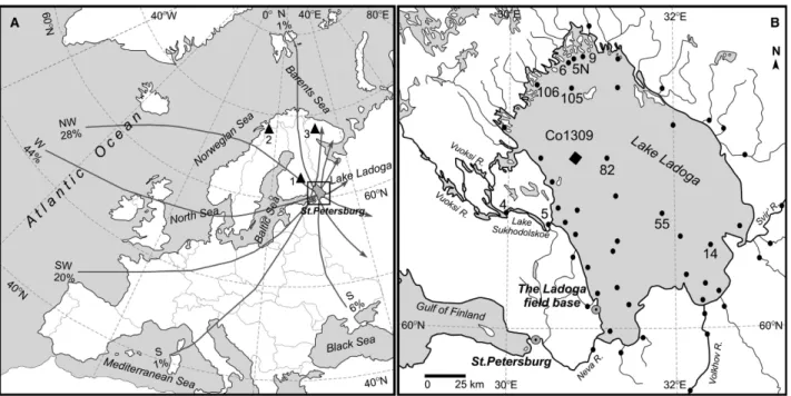
Lake Ladoga (latitude 59°54⁰–61°47⁰N, longitude 29°47⁰– 32°58⁰E, altitude 5 m a.s.l.) is a dimictic, freshwater lake located in northwest Russia,~40 km east of St. Peters- burg (Fig. 1A). The lake surface area is 18 329 km², with a mean and maximum water depth of 48.3 and 235.0 m, respectively (Rumyantsev 2015). The lake occupies an ancient tectonic and glacially sculpted depression orien- tated north-northwest to south-southeast (Fig. 1B). The

Fig. 1. A. Schematic maps showing the Lake Ladoga region with typical trajectories for cyclones modified from Shveret al.(1982) and M€atlik &

Post (2008). Locations of Lake Saarikko (southeast Finland), Lake 850 (Swedish Lapland), Lake Chuna (Kola Peninsula, northwest Russia) mentioned in the text are given (black triangles 1, 2 and 3, respectively). B. Location of Lake Ladoga (59°54⁰–61°47⁰N; 29°47⁰–32°58⁰E, 5 m a.s.l.) with the position of the Co 1309 sediment core (black diamond) and the water sampling sites (black circles, numbers indicate positions mentioned in the text); as well as location of the Losevskaya channel and modern River Burnaya (numbers 4 and 5, respectively).

(3)

basin comprises metasediments with effusive and sedimentary rocks of Archean to Cambrian age, overlain by thick Quaternary deposits (Subetto et al. 1998; Sha- balina et al. 2004; Subetto 2009; Rumyantsev et al.

2015). Lake bathymetry is broadly defined by a deep northern sector (70–235 m) that gradually shallows to the south (3–13 m) (Rumyantsev 2015). Numerous fjords and islands characterize the northern region of the lake, while large and shallow open bays occupy the southern shores.

The lake is a hydrologically open system with a water residence time of c. 11 years and a catchment area of 258 600 km² (Kimstach et al. 1998; Subetto 2009;

Rumyantsev 2015; Rumyantsevet al.2015). Lake Lad- oga receives water from numerous rivers including three main inflows: (i) the Svir’(34%) entering the lake from the east, (ii) the Vuoksi (27%) from the west; and (iii) the Volkhov (23%) from the south (Subetto et al. 1998;

Rumyantsev 2015). The River Neva outflows from the southwest of the lake into the Gulf of Finland (Fig. 1B).

The lake water balance has been shown to predominantly reflect the inflow from rivers and streams (~85%), as well as direct input from precipitation (~10%). Groundwater inputs are insignificant (Kimstachet al.1998; Shabalina et al.2004; Rumyantsev & Kondratyev 2013). Mean lake water temperature is persistently low,c. +6 °C. Mean surface water (0–10 m depth) temperature can reach +16 °C in August (Rumyantsev 2015). The lake is typically ice-covered for more than half the year from early November to ice-out in late May (Karetnikov & Naumenko 2008). However, occasionally incomplete freezing of Lake Ladoga may occur with areas of open water remaining in the northern part throughout the winter (Karetnikovet al.

2016).

The regional climate is transitional between maritime and continental, although westerly Atlantic air masses prevail year round (Rumyantsevet al.2015). Average annual air temperature in the Lake Ladoga region is+3.2°C, ranging from8.8 °C (February) to+16.3 °C (July) (Rumyantsev

& Kondratyev 2013; Rumyantsev 2015). Annual precipitation varies spatially from 380 to 490 mm in the northwest region of the lake, to 500–630 mm in the south. The driest months are February and March (24 mm) and the wettest is September (58 mm) (Rumyantsev & Kondratyev 2013;

Rumyantsev 2015; Rumyantsevet al.2015).

Climate in this region reflects the trajectories of the prevailing air masses. Typically, marine cyclones moving from the west, southwest or northwest (Fig. 1A; Shver et al.1982) bring cloudy, windy weather and precipitation, and cause abrupt warming in winter and cooling in summer. Conversely, dry continental air masses from the east, south or southeast induce relatively hot summers and cold winters. Incursions of dry Arctic air masses from the north (e.g. Barents Sea) and northeast (e.g. Kara Sea) are accompanied by clear weather, reduced precipitation and a sharp drop in air temperatures (Lydolph 1977; Shveret al.1982; Rumyantsevet al.2015).

Material and methods

Sediment and water recovery

A 22.7-m-long sedimentcore (Co1309)wasretrievedfrom Lake Ladoga (60°59⁰N, 30°41⁰E; water depth: 111 m;

Fig. 1B) in September 2013, using gravity and percussion piston-corers operated from a floating platform (UWI- TEC Ltd., Austria). The core was split, described and subsampled for sedimentological, biological and geochemical analyses at the University of Cologne.

Lake water samples were collected at semi-regular intervals in the water column between the surface and bottom (n= 190), at different spatial locations across the lake (Fig. 1B). Water was sampled directly from inflow and outflow rivers connected to the lake (n =61), and event-based precipitation samples (n = 57) were collected at the Ladoga field base of the Arctic and Antarctic Research Institute (AARI, St. Petersburg, Russia). All water samples were stored cool in airtight bottles prior to stable isotope analyses.

Core lithology and chronology

This study focuses on the upper 202 cm of the core Co 1309 from Lake Ladoga sediments for diatom oxygen isotope investigation. A recent lithological study on core Co 1309 (Gromiget al.in press) reported that the selected part of the core (Fig. 2A), consisting of predominantly massive silty clay (160–202 cm) and laminated clayey silt with minor occurrence of fine sand (0–

160 cm), was deposited during the lastc.11.2 cal. ka BP, i.e. it covers the whole Holocene. For the entire post- glacial succession, the age-depth model for the core Co 1309 was established on the basis of two radiocarbon dates (755970 and 2547171 cal. a BP; Fig. 2A) and an independent varve chronology, further confirmed by an OSL age of 7000300 cal. a BP at a depth of 130 cm.

The complete age-depth model for the sediment core is presented in Gromiget al.(in press). The Holocene onset is supported by the results of pollen analyses (Savelieva et al.2019).

Biogenic silica and diatom analyses

Biogenic silica (BSi) analysis was performed on 0.45 g of dry sediment sampled from Co 1309 at 16-cm intervals down core (n =14). Samples were ground and analysed for BSi using the automated sequential leaching method (M€uller & Schneider 1993) at the Alfred Wegener Institute Helmholtz Centre for Polar and Marine Research (AWI Bremerhaven, Germany). Biogenic opal was calculated from BSi assuming a 10% water content within the frustule (Mortlock & Froelich 1989; M€uller & Schneider 1993).

These 14 samples were also processed for diatom taxonomy analysis using sediment disintegration in

(4)

sodium pyrophosphate (Na₄P₂O₇10H₂O) and subsequent fraction separation in heavy liquid (specific density 2.6 g cm³) (e.g. Gleseret al.1974). Species abundance data were converted to percentages and diatom concentrations (910⁶valves g¹of dry sediment) were calculated according to the method outlined by Davydova (1985).

Taxonomic identification followed Krammer & Lange- Bertalot (1986, 1991).

Diatom preparation and purity estimation

Twenty-four sediment samples with an initial biogenic opal content (Fig. 2B) above 6% taken at 8-cm intervals and yielding an average temporal resolution of about 440 years throughout the pastc.10.8 ka were processed ford¹⁸Odiatomanalysis. Diatom purification involved a multi-step procedure based on Morleyet al.(2004). In summary, sediment samples were treated with 35% H2O2

on a heating plate at 50 °C for 3 days, before using 10%

HCl at 50°C to eliminate carbonates. Samples were then centrifuged in sodium polytungstate (SPT; 3Na2WO49- WO3H2O) heavy liquid (2.50–2.05 g cm³) at 2500 rpm for 30 min to separate diatoms from the detrital contam-

inants with higher density. This detritus was retained for a contamination assessment and d¹⁸Odiatom correction.

Purified diatoms were then washed in ultra-pure water using a 3lm filter. Finally, sampleswere wet sieved using a nylon mesh and sonication system, resulting in two diatom size fractions (3–10 and >10lm). Only the 3–10lm fraction yielded sufficient material (>1.5 mg) to be used ford¹⁸Odiatomanalysis.

To assess sample purity, the chemical composition of all diatom samples, as well as of three samples of heavy liquid-separated detrital material, was measured using energy-dispersive X-ray spectroscopy (EDS; Chapligin et al. 2012a). Measurements were performed with a ZEISS ULTRA 55 Plus Schottky-type field emission scanning electron microscope (SEM) equipped with a silicon drift detector (UltraDry SDD). The analysis was carried out using the standardless procedure (three repe- titions, an acceleration voltage of 20 kV; excited area size of 100–200lm, measuring time of 0.5 min; Chap- liginet al.2012a, b) at the German Research Centre for Geosciences (GFZ), Potsdam. The EDS data (Table 1;

Fig. 2F) indicate 19 of the 24 prepared diatom samples were exceptionally pure, comprising between 98.2 and

0 20 40 60 80 100 120 140 160 180 200

2547±171

7559±98

Silty clay Laminated clayey silt

Depth (cm)

Lithology and dates (cal. a BP)

0 1 2 3 4 5 6 7 8 9 10 11 12

Age (cal. ka BP)

0 10 20 (%) Biogenic

opal

0 90 180 (x10⁶ valves g^-1)

Total diatom concentration

0 100 0 25 0 5 0 50 5 0 5 0 5 0 50 50 5 0 5 0 5 0 5

Fragilaria capucina

Aulacoseira islandica Aulacoseira subarctica Cyclotella radiosa Cyclotella schumannii Cymbella spp. Fragilaria heidenii Staurosirella pinnata Navicula spp.

Stephanodiscus medius S. minutulus S. neoastraea Tabellaria fenestrata

Diatom abundance (%)

29 31 33 35

Diatom zoneDZ-1DZ-2

18O diatom

95 100 (%)

0 2

(%) Concentration

in diatoms SiO₂ Al₂O₃

A B C D E F

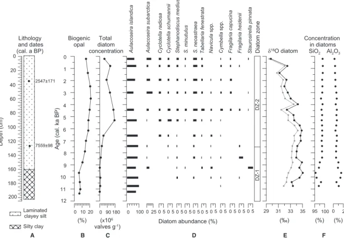
Fig. 2. Summary data from Lake Ladoga Co 1309 core. A. Sediment lithology and radiocarbon dates (Gromiget al.in press). B. Biogenic opal. C.

Total diatom concentration. D. A simplified diatom taxonomy diagram. E. Measuredd¹⁸Omeas(grey line), contamination-correctedd¹⁸Ocorrvalues of diatoms (bold black line). F. SiO2and Al2O3concentrations of the purified diatom samples analysed by EDS and measured ford¹⁸O.

(5)

99.1% SiO2, and 0.2–0.7% Al2O3; and five samples were less pure with 95.4–97.1% SiO2, and 0.9–1.4% Al2O3. In general, all samples contained<2.5% Al2O3(Chapligin et al.2012a) and hence, were analysed ford¹⁸Odiatom.

Diatom isotope analysis andd¹⁸Odiatomcorrection Purified diatom samples (n =24) and the detrital con- taminant subsamples (n =3) were analysed ford¹⁸O at AWI Potsdam. Samples were placed inside an inert gas flow dehydration (iGFD) chamber and heated to 1100°C under argon gas to remove exchangeable oxygen (Chapliginet al.2010). Dehydrated samples were then fully reacted using laser fluorination with a BrF5reagent to liberate O2 (Clayton & Mayeda 1963) and directly measured against an oxygen reference sample of known isotopic composition with a PDZ Europa 2020 mass spectrometer. Replicate analyses of the calibrated work- ing standard BFC (Chapliginet al.2011) yieldedd¹⁸O= +28.730.18& (n = 31) indicating an accuracy and analytical reproducibility within the method’s long-term analytical reproducibility (1r) of 0.25& (Chapligin et al.2010).

All measured diatomd¹⁸O values were contamination corrected using the geochemical mass-balance approach (Swann & Leng 2009; Chapliginet al.2012a, b):

d¹⁸O_corr¼ ðd¹⁸O_measd¹⁸O_cont

ccont=100Þ=ðc_diatom=100Þ ð1Þ

whered¹⁸Omeasis the original measuredd¹⁸O value of the sample.d¹⁸Ocorris the measuredd¹⁸O value corrected for contamination, with d¹⁸Ocont = +12.80.6& (n = 3), which represents the averaged¹⁸O of the heavy detrital fractions after the first heavy liquid separation. The percentages of contamination (ccont) and diatom material (cdiatom) within the analysed sample are calculated using the EDS-measured Al2O3content of the individual sample divided by the average Al2O3 content of the contamination (14.80.9% in heavy fractions, n = 3) and as (100%–ccont), respectively.

Stable water isotope analysis

Water samples were measured for oxygen (d¹⁸O) and hydrogen (dD) isotopes at the AARI using a Picarro L2120-i (n = 281) and at AWI Potsdam with a Finnigan MAT Delta-S mass spectrometer (n = 7). At the AARI, sequences of measurements included the injection of five samples, followed by the injection of an internal labo- ratory standard with an isotopic composition close to that of the samples. Replicate measurements on 10% of all samples indicate an analytical precision of 0.30&for dD and 0.06& for d¹⁸O. AWI measurements were performed using equilibration techniques and yield an analytical uncertainty (1r) of0.8&fordD and0.1&

ford¹⁸O (Meyeret al.2000). The secondary parameter deuterium excess is calculated as d= dD – 8 d¹⁸O (Dansgaard 1964), and all values are reported in per mil

Table 1.Main geochemical characteristics of diatoms from Lake Ladoga based on EDS data. Measuredd¹⁸O values (d¹⁸Omeas), calculated contamination (ccont) andd¹⁸O values corrected for contamination (d¹⁸Ocorr) are given.

Core Sample

depth (cm)

Age (cal.

ka BP) SiO2

(%)

Al2O3

(%)

Na2O (%)

MgO (%)

K2O (%)

CaO (%)

MnO (%)

FeO (%)

Total d¹⁸Omeas

(&)

ccont

(%)

d¹⁸Ocorr

(&)

Co1309-14-III 3 0.203 98.98 0.23 0.55 0.10 0.02 0.06 0.01 0.05 100.00 29.49 1.6 29.76

Co1309-14-III 11 0.793 99.08 0.35 0.33 0.04 0.03 0.04 0.04 0.10 100.00 32.03 2.4 32.49

Co1309-14-III 19 1.373 99.05 0.34 0.30 0.04 0.03 0.10 0.03 0.11 100.00 30.76 2.3 31.18

Co1309-14-III 27 1.939 98.77 0.41 0.37 0.08 0.06 0.08 0.03 0.19 100.00 31.79 2.8 32.33

Co1309-14-III 35 2.483 98.89 0.43 0.32 0.07 0.06 0.03 0.04 0.16 100.00 31.44 2.9 32.00

Co1309-14-III 43 3.001 98.80 0.61 0.19 0.07 0.09 0.06 0.03 0.16 100.00 31.74 4.1 32.56

Co1309-14-III 51 3.495 98.17 0.68 0.58 0.13 0.10 0.07 0.04 0.23 100.01 32.11 4.6 33.04

Co1309-14-III 59 3.969 98.95 0.48 0.21 0.07 0.01 0.09 0.06 0.14 100.00 33.53 3.3 34.23

Co1309-14-III 67 4.425 98.44 0.70 0.25 0.10 0.06 0.11 0.07 0.27 100.00 31.48 4.7 32.41

Co1309-14-II 75 4.868 98.73 0.62 0.21 0.09 0.10 0.08 0.03 0.16 100.01 32.64 4.2 33.51

Co1309-14-II 83 5.301 98.54 0.71 0.23 0.10 0.03 0.11 0.06 0.22 100.00 32.62 4.8 33.62

Co1309-14-II 91 5.727 98.70 0.59 0.34 0.06 0.04 0.08 0.05 0.15 100.00 33.67 4.0 34.54

Co1309-14-II 99 6.150 98.74 0.43 0.46 0.08 0.06 0.04 0.04 0.16 100.00 34.22 2.9 34.86

Co1309-14-II 107 6.574 98.79 0.70 0.13 0.07 0.02 0.05 0.03 0.21 100.00 33.62 4.7 34.65

Co1309-14-II 115 7.001 98.50 0.70 0.40 0.10 0.06 0.07 0.04 0.15 100.01 33.67 4.7 34.71

Co1309-14-II 123 7.437 98.70 0.58 0.25 0.10 0.03 0.08 0.02 0.23 100.00 33.31 3.9 34.15

Co1309-14-II 131 7.883 98.68 0.55 0.35 0.11 0.03 0.06 0.03 0.19 100.00 33.24 3.7 34.03

Co1309-14-I 140 8.394 98.72 0.55 0.22 0.13 0.06 0.11 0.01 0.21 100.01 33.18 3.7 33.97

Co1309-14-I 147 8.790 97.58 1.02 0.28 0.27 0.11 0.16 0.02 0.57 100.00 33.38 6.9 34.91

Co1309-14-I 155 9.235 97.13 0.93 0.85 0.27 0.13 0.13 0.07 0.50 100.00 33.11 6.3 34.48

Co1309-14-I 163 9.662 95.42 1.58 0.80 0.69 0.28 0.07 0.02 1.14 100.00 32.66 10.7 35.05

Co1309-14-I 171 10.062 95.95 1.42 0.65 0.64 0.26 0.12 0.01 0.95 100.00 32.42 9.6 34.51

Co1309-3-II 179 10.428 98.15 0.63 0.58 0.14 0.10 0.12 0.05 0.24 100.00 32.34 4.3 33.21

Co1309-3-II 187 10.750 97.07 1.09 0.57 0.38 0.15 0.11 0.03 0.61 100.01 31.89 7.4 33.41

(6)

(&) difference relative to Vienna Standard Mean Ocean Water (VSMOW).

Results

Holocene diatom flora

Diatom frustules in core Co 1309 are well preserved down core and 118 different lacustrine taxa were iden- tified in the Holocene. No marine or brackish taxa were observed in the upper 201 cm (11.18 cal. ka BP). An exception is the lowermost part, where negligible amounts of reworked Eemian marine diatoms are present. However, these samples did not contain sufficient biogenic opal for purification and diatom isotope analyses.

Two main diatom zones (DZs) are defined in the record based on species diversity and diatom concentration (Fig. 2C, D).

DZ-1 (202–125 cm;c.11.2–7.5 cal. ka BP) is dominated by planktonicAulacoseira islandica(O. M€ull.) Sim.

(85–95%). The abundances of other planktonic Aula- coseira subarctica(O. M€ull.) E.Y. Haw.,Stephanodiscus spp., Tabellaria fenestrata(Lyngb.) K€utz. and benthic Cymbella spp., Fragilaria spp. sensu lato, Navicula spp. do not exceed 1–2% (Fig. 2D). An exception is the interval from 145 to 165 cm (c.8.7–9.8 cal. ka BP), where the relative abundance ofA. islandicadecreases to 72%, while planktonic A. subarctica and epiphytic Stau- rosirella pinnata (Ehr.) Will. & Round and Fragilaria heidenii (Østr.) abundances increase to 9, 5 and 4%, respectively. Negligible amounts of Chaetoceros spp.

(resting spores) and more sporadicallyCoscinodiscusspp.

andThalassiosira gravidaCl. reworked from marine Eemian sediments are observed at 202 cm (c. 11.2 cal. ka BP).

Diatom concentration in this zone is low, reaching a maximum of 24.8910⁶valves g¹at 125 cm (Fig. 2C).

DZ-2 (125–0 cm;c.7.5–0 cal. ka BP) is further dominated byA. islandica(51–91%).A. subarcticais another dominant taxon at some levels with abundances between 0.6 and 22% (Fig. 2D). The abundances of planktonic Cyclotella radiosa(Grun.) Lemm.,C. schumannii(Grun.) Hak.,Stephanodiscus mediusHak.,S. minutulus(K€utz.) Round, S. neoastraea Hak. & Hick., and T. fenestrata range between 1 and 4%. In the interval 45–70 cm (3.1–

4.6 cal. ka BP), the relative abundances of A. islandica decrease to its minimum of 51% whereasA. subarctica reaches its maximum of 22%. A sharp increase up to 14%

in the abundance of the benthic taxa, e.g.Cymbellaspp., F. capucina Desm. et vars., F. heidenii, Navicula spp., occurs at 67 cm (4.4 cal. ka BP). Over the pastc.3.1 cal.

ka BP, the relative abundance ofA. islandicaincreases to 75% at 11 cm (c.0.8 cal. ka BP) and then decreases to 59%

at 3 cm (c.0.2 cal. ka BP) (Fig. 2D). Total diatom concentration in DZ-2 is considerably higher than in DZ-1, peaking at 83 cm (c.5.3 cal. ka BP) with 173910⁶valves

g¹, before decreasing to 55910⁶valves g¹in the upper- most sample (Fig. 2C).

Holocene oxygen isotope record

Holocened¹⁸Ocorrvalues in Lake Ladoga range between +29.8 and+35.0&(mean:+33.5&) (Fig. 2E; Table 1).

Diatomd¹⁸Ocorrvalues (further referred to asd¹⁸Odiatom) exhibit the same trend asd¹⁸Omeasvalues, but due to the contamination correction are, on average, about 0.8&

higher in the upper part of the core (younger than 8.8 cal.

ka BP) and approximately 1.8&higher for the lower part (older than 8.8 cal. ka BP).

Between c.10.7 and 10.4 cal. ka BP, d¹⁸Odiatom are relatively low, around +33.2&. After 10.2 cal. ka BP values steadily increase, attaining a Holocened¹⁸Odiatom

maximum at 9.6 cal. ka BP (+35.0&). After 9.6 cal. ka BPd¹⁸Odiatomvalues slightly decrease to+34.0&, before increasing to a second maximum of+34.9&atc.6.1 cal.

ka BP. A sharp drop to+32.4&atc.4.4 cal. ka BP and subsequent rise to +34.2& at c. 4.0 cal. ka BP in d¹⁸Odiatom are observed. The Late Holocene interval betweenc.4.0 and 0.2 cal. ka BP exhibits a continuous decrease of 4.4& in d¹⁸Odiatom values, reaching the Holocene minimum of +29.8 & at c. 0.2 cal. ka BP.

However, there are two local maxima with +32.3 and

+32.5&atc. 1.9 and 0.8 cal. ka BP, respectively. Overall,

the record exhibits a continuous gradual d¹⁸Odiatom

depletion of ~0.55& per 1000 years from the Early Holocene to the sediment surface with an accelerated depletion of~1.1&per 1000 years afterc.4.0 cal. ka BP (Fig. 2E).

Water isotopes

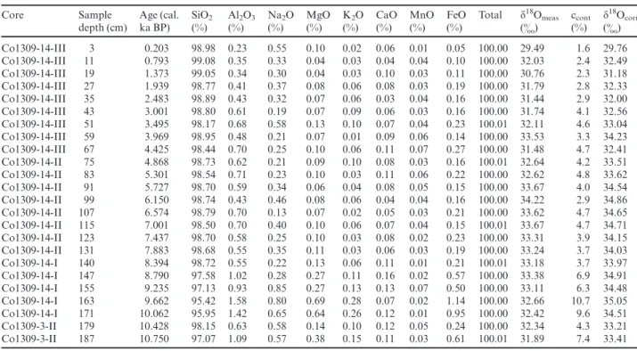
Stable water isotope data (d¹⁸O, dD andd excess) are presented in Fig. 3 and summarized in Table 2.

The modern Lake Ladoga water isotope composition varies between –10.3 and –9.2& (mean: 9.8&) for d¹⁸Olakeand from78.2 to71.8&(mean:75.5&) for dDlake.dexcess values range from+1.5 to+5.5&(mean:

+3.1&). In the northern part of the lake,d¹⁸Olakevalues

range between10.2 and 9.7& (mean:–9.9&) and dDlakefrom76.7 to74.9&(mean:75.8&).dexcess ranges from+2.2 to+5.5&(mean:+3.3&). The southern basin has similar isotopic composition that ranges between10.3 and9.2&(mean:9.8&) ford¹⁸Olake

and from78.1 to71.8&(mean:75.1&) fordDlake.d excess ranges from+1.8 to+4.6&(mean:+3.0&). Water column d¹⁸O profiles reveal no substantial changes with depth, with a maximum range of0.4&(Fig. 4).

Similarly, the inflow rivers exhibit mean values of9.8, 74.8 and+3.8&ford¹⁸O,dD anddexcess, respectively (n = 39). The outflow (Neva River) displays slightly higher mean values of9.6&ford¹⁸O, and74.2&fordD (d excess:+2.7&).

(7)

Precipitation sampled at Lake Ladoga between July and December is characterized by mean values of7.6&for d¹⁸O and55.7&fordD (dexcess+5.3&). Precipitation samples were not collected during the rest of the year.

Discussion

Modern water isotope hydrology

Thed¹⁸Olakeis affected by precipitation and additional hydrological parameters (i.e. evaporation and inflow/

outflow ratio), and hence, assumed to be one of the main controls on the lacustrine d¹⁸Odiatom (Leng & Barker 2006). Therefore, the modern isotope hydrology of Lake Ladoga has been comprehensively assessed and compared to regional precipitation (own samples (Table 2) and Global Network of Isotopes in Precipitation (GNIP), St. Petersburg) as background information for thed¹⁸Odiatominterpretation.

Stable isotope data for precipitation collected on the western shore of Lake Ladoga (field base; Fig. 1B) dis- play clear seasonal variations with higher meand¹⁸Oprec, dD_precanddexcess values of8.8,62.8 and+7.3&, respectively, in summer (June–August) and lower mean values of13.4,99.8 and+4.8&, respectively, in Dec- ember (Table 2). Thed¹⁸O–dD relationship for collected precipitation is characterized by a slope of 7.7 and intercept of +4.3 (R²= 0.98; Table 2), slightly higher than the respective values for the Local Meteoric Water Line (LMWL; Fig. 3;dD= 7.2d¹⁸O–1.5;R²= 0.87;

GNIP database; IAEA/WMO 2018).

In contrast, the isotopic composition of the Lake Ladoga water varies in a relatively narrow range around average values of9.8&ford¹⁸O_lake,75.5&fordD_lake and a meandexcess of+3.1&(Table 2). These values are in good agreement with those of the rivers (meand¹⁸O=

9.8&;dD = 74.8&anddexcess= +3.8&; Table 2;

n = 39) draining into the lake. Lake Ladoga water isotope samples are situated below the GMWL (Fig. 3A), and follow a linear dependence with a slope of 4.8 and an intercept of28.5 (R²= 0.82), suggesting that the lake water is substantially influenced by evaporative enrichment. The intersection point of this evaporation line (EL) and the GMWL is at about12.0&for d¹⁸O and at86.0&fordD and, hence, quite similar to the weighted mean annual isotope composition of precipitation in St. Petersburg of 11.4 and87.2&

ford¹⁸OprecanddDprec, respectively (1980–1990, IAEA/

WMO 2018). This is slightly lower than the mean isotopic composition of the inflow rivers (Table 2), suggesting that Lake Ladoga is predominantly fed by meteoric waters, i.e. precipitation with an important riverine contribution. The share of river water and precipitation in the water balance of the lake is about 85 and 10%, respectively (Rumyantsev 2015). Evaporation may comprise about 8% of the annual output from Lake Ladoga (Rumyantsev & Kondratyev 2013) and is likely to be seasonally related to the lake ice cover.

Lake Ladoga receives water from numerous rivers (Subettoet al.1998; Rumyantsev 2015). Thed¹⁸Olakeand dDlakevalues for Lake Ladoga in the inflow area of River Svir’are10.3 and77.9&, respectively, and, thus this area has an isotope composition similar to that of River Svir’(Table 2). River Vuoksi flows into Lake Ladoga by a northern and a southern tributary (through Losevs- kaya channel, Lake Sukhodolskoe and modern River Burnaya; Fig. 1B; Rumyantsev & Kondratyev 2013).

The average isotope composition of the lake water in A

B

Fig. 3. d¹⁸O–dD diagram for water samples. A. Lake Ladoga and rivers connected to the lake as well as precipitation (compare with Table 2). B.

Lake Ladoga hydrology. Additionally, the Global Meteoric Water Line (GMWL;dD=8d¹⁸O+10; Craig 1961; Rozanskiet al.1993) and Local Meteoric Water Line (LMWL) based on GNIP data (IAEA/

WMO 2018) as well as an evaporation line (EL) for Lake Ladogawaters are given.

(8)

both areas influenced by rivers Vuoksi and Burnaya is 9.8&ford¹⁸O and75.4&fordD (dexcess of+2.8&) and close to the isotope composition of the connected riverine inflows (Table 2). Average values for rivers Vuoksi and Svir’fall into the field of isotope composition of the lake water (Fig. 3B). Notably heavier isotope compositions of about 1&ford¹⁸O and about 8&fordD are observed for River Volkhov aswell as for lake water near the Volkhov inflow probably because of River Volkhov draining the southern part of the Ladoga catchment.

Despite this, the average lake isotope composition in the area of the River Volkhov mouth is9.6&ford¹⁸O and 74.1&fordD (dexcess= +2.9&), and in general compa- rable with the mean values for Lake Ladoga (Table 2), indicating that Volkhov River has a negligible influence on the overall water isotope balance of the lake. Rumyantsev &

Kondratyev (2013) also observe significant differences in the ion content of Lake Ladoga and River Volkhov waters, supporting this assumption.

Consequently,d¹⁸OlakeanddDlakecan, theoretically, be fully explained by water input of rivers Vuoksi and Svir’, with a smaller contribution from Volkhov. How- ever, as both river and lake water samples are situated below the LMWL (Fig. 3B), evaporative effects are very likely both in the catchment and in the lake itself. As compared to the most important inflow Svir’, the western Vuoksi river displays a distinctly more evaporative isotope signature, probably due to its drainage through several shallow waterbodies (Rumyantsev &

Kondratyev 2013). The calculated share of losses through evaporation from the Ladoga catchment in summer is substantial, and has been estimated at 23%

(Rumyantsevet al.2017). The river waters draining into Lake Ladoga are distributed all over the lake due to efficient mixing processes. Nonetheless, the river input cannot significantly change the average isotope composition of the lake water within a single year. The total river discharge into the lake of about 71 km³a¹(Holopainen

& Letanskaya 1999) is 10 times lower compared to the whole volume of Lake Ladoga of ~848 km³ (Rumyantsevet al.2015). Additionally, no large offsets between the lake and river water samples entering the lake (slope and intercept are 5.9 and16.6, respectively;

Table 2) are notable (Fig. 3B).

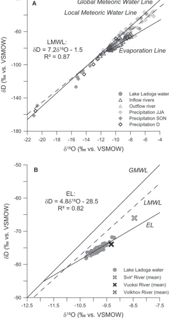
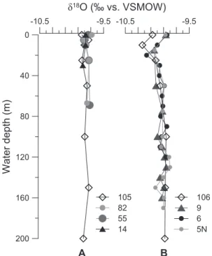
Lake Ladoga d¹⁸O-depth profiles exhibit a narrow range of 0.2& (Fig. 4A), thereby indicating a well- mixed water column with no isotopic stratification. An intensive full vertical mixing of water-masses usually occurs twice a year during intensive spring warming and autumn cooling (Tikhomirov 1982; Malm & J€onsson 1994; Rumyantsev 2015). However, there are minor dissimilarities of 0.1–0.2& in d¹⁸O values of the lake water depending on the sampling period. Late summer lake water of 2015 (Fig. 4A) displays a slightly lower isotope composition with average values of9.9&for d¹⁸O,75.6&fordD and a slightly higher meandexcess of+3.3&as compared to early summer lake water of

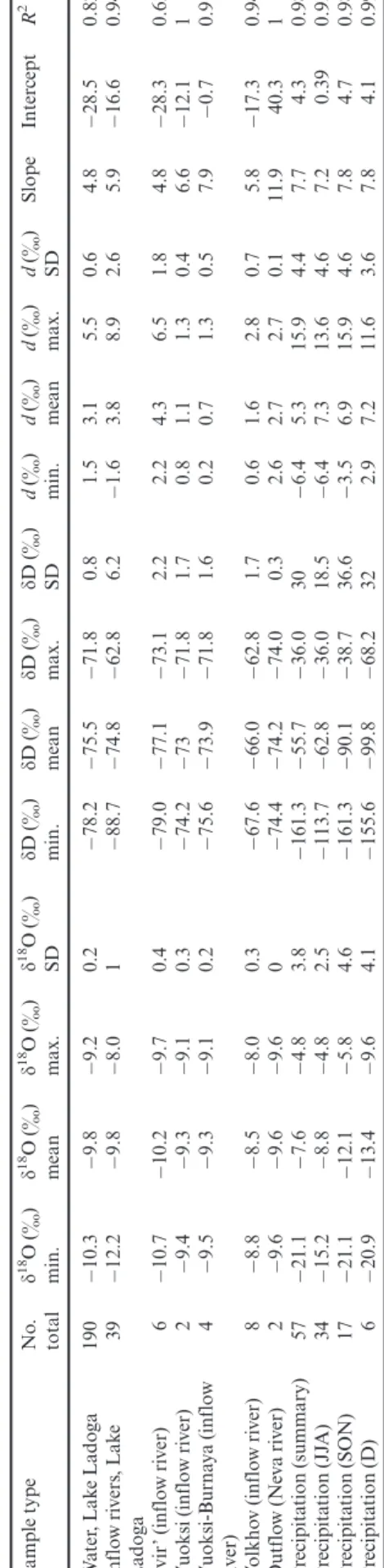
Table2.Summaryofstableisotopedata(d18O,dDanddexcess),includingminimum,meanandmaximumvalues,standarddeviations(SD)aswellasslopesandinterceptsfromthed18O–dDdiagram fortheanalysedsamplesofLakeLadogawater(collectedinAugust2015,JuneandSeptember2016),waterfromriversconnectedtoLakeLadoga(collectedinAugustandOctober2015,June2016)and precipitationwater(collectedinJuly–December2015;June–August2016). SampletypeNo. totald18O(&) min.d18O(&) meand18O(&) max.d18O(&) SDdD(&) min.dD(&) meandD(&) max.dD(&) SDd(&) min.d(&) meand(&) max.d(&) SDSlopeInterceptR2 Water,LakeLadoga19010.39.89.20.278.275.571.80.81.53.15.50.64.828.50.82 Inflowrivers,Lake Ladoga3912.29.88.0188.774.862.86.21.63.88.92.65.916.60.94 Svir’(inflowriver)610.710.29.70.479.077.173.12.22.24.36.51.84.828.30.63 Vuoksi(inflowriver)29.49.39.10.374.27371.81.70.81.11.30.46.612.11 Vuoksi-Burnaya(inflow river)49.59.39.10.275.673.971.81.60.20.71.30.57.90.70.9 Volkhov(inflowriver)88.88.58.00.367.666.062.81.70.61.62.80.75.817.30.94 Outflow(Nevariver)29.69.69.6074.474.274.00.32.62.72.70.111.940.31 Precipitation(summary)5721.17.64.83.8161.355.736.0306.45.315.94.47.74.30.98 Precipitation(JJA)3415.28.84.82.5113.762.836.018.56.47.313.64.67.20.390.95 Precipitation(SON)1721.112.15.84.6161.390.138.736.63.56.915.94.67.84.70.98 Precipitation(D)620.913.49.64.1155.699.868.2322.97.211.63.67.84.10.99

(9)

2016 (Fig. 4B) with9.7,74.8 and+2.7&ford¹⁸O,dD anddexcess, respectively. The spatial variability in the isotope signature of Lake Ladoga is also low (0.1&), ranging from9.90.1&(d¹⁸Olake;n = 77) and75.8

0.4& (dDlake) in the northern basin, to 9.80.2&

(d¹⁸O_lake;n = 52) and75.11.2&(dD_lake) in the southern part.

In summary, Lake Ladoga shows a well-mixed and temporally and spatially rather uniform isotope signature that reflects local precipitation and riverine inflow, and both river and lake water underwent notable evaporative enrichment.

Ecological and species effects

Despite a few reworked Eemian marine diatoms, which were only found at the very beginning of the Holocene at c.11.2 cal. ka BP, diatom analysis revealed the complete absence of brackish and marine diatom species in the analysed Holocene part of the Co 1309 core. This means that Lake Ladoga (at the coring position) existed as a freshwater reservoir at least for the lastc.10 800 years, an interpretation that is further substantiated by diatom isotope analyses.

Diatom species changes may have the potential to aff- ectd¹⁸Odiatombecause of (i) differences in habitats and/or blooming periods of taxa and (ii) species-specific fractionation effects (e.g. Chapliginet al.2012a). The freshwater planktonicAulacoseira islandicais the main primary producer in both modern (Holopainen & Letan-

skaya 1999; Letanskaya & Protopopova 2012) and palaeo-Lake Ladoga (Fig. 2D). During May–June, this taxon forms a biomass of up to 4.4 g m³in the photic zone when turbulence is high and the water temperature range is 5–8 °C (Letanskaya & Protopopova 2012). A secondary bloom with A. islandicatypically occurs in autumn, but the produced biomass does not exceed 1 g m³ (Letanskaya & Protopopova 2012). In summer, when Tlakecan reach 16°C (Rumyantsev & Kondratyev 2013; Rumyantsev 2015), diatoms are scarce and mainly occur in areas influenced by rivers (Holopainen & Letan- skaya 1999).

As diatom production mainly occurs in the late spring–

early summer,d¹⁸Odiatomshould reflect early seasond¹⁸Olake, possibly influenced by isotopically depleted snow-melt.

In contrast, summer–autumnd¹⁸Olakewould be dominated by the composition of summer precipitation and evaporative enrichment. However, as seasonal variations in the isotope composition of Lake Ladoga water are relatively low (Fig. 4), any possible effects ofd¹⁸Olake

seasonality ond¹⁸Odiatomare also assumed to be low.

There is no notable relationship between d¹⁸Odiatom

and species assemblage trends during the Holocene (Fig. 2D, E). Hence, considering the Holocene sediment succession is dominated by A. islandica (up to 98%), we assume that species effects have negligible impact on the isotopic signal at Lake Ladoga. This assumption is valid considering that existing studies have demonstrated no visible species composition effects on lacustrine d¹⁸Odiatom(Chapligin et al.2012a; Bailey et al.2014). Therefore, we conclude that the obtained Holocene d¹⁸Odiatom values mainly reflect conditions during theA. islandicabloom, which typically occurs in late spring/early summer.

Isotope fractionation and controls ond¹⁸Odiatom

Lake water temperature (Tlake) andd¹⁸Olakeare the main controls affecting d¹⁸O_diatom (Labeyrie 1974; Juillet- Leclerc & Labeyrie 1987; Brandrisset al.1998; Leng &

Barker 2006; Dodd & Sharp 2010).

Using the isotope fractionation between fossil diatom silica and water introduced by Juillet-Leclerc & Labeyrie (1987):

1000lna_ðsilicawaterÞ¼3:2610⁶=T²þ0:45 ð2Þ where the fractionation coefficienta(silica-water)=(1000+ d¹⁸Odiatom)/(1000+d¹⁸Olake), we calculated the expected d¹⁸Odiatomfor recent Lake Ladoga conditions. Taking (i) the meand¹⁸Olakeof–9.8&and (ii) the lake temperature range between 5 and 16 °C (Letanskaya & Protopopova 2012; Rumyantsev & Kondratyev 2013; Rumyantsev 2015), expected recentd¹⁸Odiatomvalues (Fig. 5A) range between+30.0 and+33.3&(meand¹⁸Odiatom= +31.6&).

As the main diatom bloom dominated byA. islandica occurs at Tlakeof 5–8 °C (Letanskaya & Protopopova

Fig. 4. Water isotope depth profiles at different locations in the lake. A.

In the northern (105), central (55; 82) and southern (14) parts (sampled in June 2016). B. In the northern deeper part (106; 9; 6; 5N sampled in August 2015).

(10)

2012), the expected recent d¹⁸O_diatom values can be further constricted to values between+32.3 and+33.3&

(Fig. 5A). As this range generally matches the range of the Holocene d¹⁸Odiatom values at Lake Ladoga, we assume that ourd¹⁸Odiatomdata are in the right order of magnitude.

When considering a temperature coefficient of0.2&

per°C (Swann & Leng 2009; Dodd & Sharp 2010), the overall~4&Holocene decrease ind¹⁸Odiatom(Fig. 2E) would result in an unrealistic late spring/summer Tlake

change of~20 °C (which would yield negative Tlakein the Early Holocene). Hence, Tlakealone cannot be the primary controlling factor on Lake Ladogad¹⁸Odiatom. Instead, we propose that changes in d¹⁸Olake are the primary control ond¹⁸Odiatomin Lake Ladoga, as observed in similar studies elsewhere (e.g. Kostrovaet al.2013; Meyer et al.2015; Baileyet al.2018). These changes ind¹⁸Olake

originate either from isotopic variations in precipitation (d¹⁸Oprec) and/or from changes in the hydrological conditions.

Both air temperature (T_air) and the pathways of atmospheric moisture are major impact factors on d¹⁸Oprec (Dansgaard 1964; Clark & Fritz 1997). The relationship between monthly meand¹⁸Oprecand Tairfor St. Petersburg has been determined asd¹⁸Oprec=0.18 T_air–12.3 (R² =0.81) (IAEA/WMO 2018). This isotope– temperature relationship of 0.18&per°C for the Lake Ladoga region coincides well with the gradient of 0.17&

per°C calculated for marine stations (Rozanski et al.

1993; Clark & Fritz 1997) and indicates the prevalence of maritime air masses from the Atlantic to the region’s water balance. Consequently, this relatively low positive Tair–d¹⁸Oprecgradient would be largely counterbalanced by the negative Tlake–d¹⁸Oprecrelationship. Taking into account that Tairat Lake Ladoga (monthly means from 8 to+16 °C) varies by a factor ofc.2 more than Tlake(5– 16°C), Tair will be always more effective than Tlake. Hence, we conclude that (i) lake temperatures will fully be counterbalanced by air temperature changes; (ii) Tair

changes probably have little effect ond¹⁸Olake, and hence

A B

F

C D E

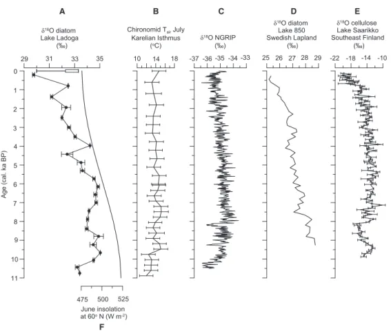
Fig. 5. Holocene palaeoenvironmental comparison. A. Contamination-correctedd¹⁸Odiatomrecord from Lake Ladoga (this study) and expected range of recentd¹⁸Odiatomvalues calculated for Tlakebetween 5 and 16°C using the correlation of Juillet-Leclerc & Labeyrie (1987); the open rectangle represents the expectedd¹⁸Odiatomfor theAulacoseira islandicablooming period at Tlakeof 5–8°C. B. July air temperatures reconstructed from chironomids in Karelian Isthmus (Nazarovaet al.2018). C. NGRIPd¹⁸O record from Greenland (Svenssonet al.2008) as an indicator of the Northern Hemisphere air temperatures. D.d¹⁸Odiatomrecord from Lake 850, Swedish Lapland (Shemeshet al.2001). E.d¹⁸Ocelluloserecord from Lake Saarikko, southeast Finland (Heikkil€aet al.2010). F. Northern Hemisphere summer insolation at 60°N (Berger & Loutre 1991).