Water isotopes – climate relationships for the mid-Holocene and preindustrial period simulated with an isotope-enabled

(1)

https://doi.org/10.5194/cp-15-1913-2019

Water isotopes – climate relationships for the mid-Holocene and preindustrial period simulated with an isotope-enabled

version of MPI-ESM

Alexandre Cauquoin, Martin Werner, and Gerrit Lohmann

Alfred Wegener Institute, Helmholtz Centre for Polar and Marine Sciences, Bremerhaven, Germany Correspondence:Alexandre Cauquoin (alexandre.cauquoin@awi.de)

Received: 17 June 2019 – Discussion started: 20 June 2019

Revised: 10 October 2019 – Accepted: 11 October 2019 – Published: 14 November 2019

Abstract. We present here the first results, for the preindustrial and mid-Holocene climatological periods, of the newly developed isotope-enhanced version of the fully coupled Earth system model MPI-ESM, called hereafter MPI- ESM-wiso. The water stable isotopes H¹⁶₂ O, H¹⁸₂ O and HDO have been implemented into all components of the coupled model setup. The mid-Holocene provides the opportunity to evaluate the model response to changes in the seasonal and latitudinal distribution of insolation induced by different orbital forcing conditions. The results of our equilibrium simulations allow us to evaluate the performance of the isotopic model in simulating the spatial and temporal variations of water isotopes in the different compartments of the hydrological system for warm climates. For the preindustrial climate, MPI-ESM-wiso reproduces very well the observed spatial distribution of the isotopic content in precipitation linked to the spatial variations in temperature and precipitation rate. We also find a good model–data agreement with the observed distribution of isotopic composition in surface seawater but a bias with the presence of surface seawater that is too ¹⁸O-depleted in the Arctic Ocean. All these results are improved compared to the previous model version ECHAM5/MPIOM. The spatial relationships of water isotopic composition with temperature, precipitation rate and salinity are consistent with observational data. For the preindustrial climate, the interannual relationships of water isotopes with temperature and salinity are globally lower than the spatial ones, consistent with previous studies. Simulated results under mid-Holocene conditions are in fair agreement with the isotopic measurements from ice cores and continental speleothems. MPI-ESM-wiso simulates a decrease in

the isotopic composition of precipitation from North Africa to the Tibetan Plateau via India due to the enhanced monsoons during the mid-Holocene. Over Greenland, our simulation indicates a higher isotopic composition of precipitation linked to higher summer temperature and a reduction in sea ice, shown by positive isotope–temperature gradient. For the Antarctic continent, the model simulates lower isotopic values over the East Antarctic plateau, linked to the lower temperatures during the mid-Holocene period, while similar or higher isotopic values are modeled over the rest of the continent. While variations of isotopic contents in precipitation over West Antarctica between mid-Holocene and preindustrial periods are partly controlled by changes in temperature, the transport of relatively¹⁸O-rich water vapor near the coast to the western ice core sites could play a role in the final isotopic composition. So, more caution has to be taken about the reconstruction of past temperature variations during warm periods over this area. The coupling of such a model with an ice sheet model or the use of a zoomed grid centered on this region could help to better describe the role of the water vapor transport and sea ice around West Antarc- tica. The reconstruction of past salinity through isotopic content in sea surface waters can be complicated for regions with strong ocean dynamics, variations in sea ice regimes or significant changes in freshwater budget, giving an extremely variable relationship between the isotopic content and salinity of ocean surface waters over small spatial scales. These complicating factors demonstrate the complexity of inter- preting water isotopes as past climate signals of warm periods like the mid-Holocene. A systematic isotope model in-

(2)

tercomparison study for further insights on the model depen- dency of these results would be beneficial.

1 Introduction

The hydrogen and oxygen atoms that compose the water molecule have several natural stable isotopes. This results in several forms of the water molecule called water stable isotopologues (hereafter designated by the term “water isotopes”), the most common being H¹⁶₂ O, H¹⁸₂ O and HDO.

These water isotopes, expressed hereafter in the usualδno- tation (asδ¹⁸O andδD with respect to the Vienna Standard Mean Ocean Water V-SMOW if not stated otherwise), are integrated tracers of climatic processes occurring in diverse parts of the hydrological cycle (Craig and Gordon, 1965;

Dansgaard, 1964). Because of their differences in mass and symmetry, an isotopic fractionation happens at each phase change depending on environmental conditions. As a consequence, the water isotopes have been successfully used during the last decades to study past climate changes and to describe the present-day water cycle through their measurements in various natural archives. Many of these studies are based on a modern analog approach, i.e., by assuming that the modern spatial relationship between water isotopes and surface temperatures, precipitation amount or salinity provides a calibration that can be used for different past climates. In addition, to be consistent with the observed close relationships between water isotopic time series and temperature or precipitation amount variations, this hypothesis can be validated by a Rayleigh distillation model representing the evolution of the remaining water vapor in a cloud (i.e., loss of heavier isotopes during condensation and precipitation events) as it is transported from moisture source region to high latitudes (Ciais and Jouzel, 1994). For example, the isotopic signal measured in polar ice cores enabled at a 1st order the reconstruction of past temperature variations at high resolution (Jouzel, 2013, and references therein), allowing for the description of past climate changes over several glacial–

interglacial periods (Jouzel et al., 2007; NEEM Community Members, 2013). In the (sub)tropical areas, the δ¹⁸O in the calcite of speleothems is interpreted in terms of past monsoon dynamics (i.e., linked to the quantity of precipitation, called the “amount effect”) (Wang et al., 2001, 2008). Anal- ogously to the continental speleothems, theδ¹⁸O conserved in the carbonates of foraminifers or corals can be measured.

It is controlled by the¹⁸O isotopic composition of ocean water and the temperature at the calcite formation. Such records from marine sediment cores are essential to deduce mean sea level changes, which are linked to the global ice volume during different climates (Shackleton, 1967). Moreover, the local variations in the δ¹⁸O of ocean water tend to be dependent on changes in freshwater budget and ocean circulation, so they provide information about salinity changes. Finally, the combination ofδD andδ¹⁸O measured in the same sam-

ple gives access to the 2nd-order parameter deuterium excess (d-excess), defined as d-excess=δD−8×δ¹⁸O (Dansgaard, 1964). Deuterium-excess changes are often interpreted as a source region effect; i.e., d-excess is related to the humidity and temperature conditions at the evaporative source regions (Merlivat and Jouzel, 1979). Other processes that could drive the d-excess variability have been suggested, like the moisture source relative humidity (Pfahl and Sodemann, 2014), the moisture recycling or the evaporation of falling drops (Fröhlich et al., 2002).

However, the quantitative translation of past isotope signals recorded in natural archives to climate variables and their interpretation remains challenging because of the numerous and complex processes involved: changes in evaporation conditions and moisture sources, in atmospheric transport pathways, or in the seasonality of the precipitation. For example, using the spatial relationship between theδ¹⁸O in Greenland ice core records and surface temperature to evaluate the local temperature variations during the last deglacia- tion leads to a large uncertainty of a factor of 2 (Jouzel, 1999;

Buizert et al., 2014). This has been attributed to changes in air mass origins (Werner et al., 2001), precipitation seasonality (Krinner et al., 1997; Krinner and Werner, 2003) or to a dampening of isotopic changes by ocean evaporation (Lee et al., 2008). In East Antarctica, it has been suggested that the relationship between temperature and the isotopic signature for warmer interglacial periods can vary among ice core sites, with an error on the temperature reconstruction that can reach up to 100 % (Sime et al., 2009; Cauquoin et al., 2015).

At lower latitudes, the interpretation of water isotope records is even more complex because of the convective processes (Risi et al., 2008) and the importance of the precipitation intensity that affect the isotopic composition of these records (Vimeux et al., 2005). In the oceans, quantitative reconstruc- tions of past salinity variability based on its spatial relationship withδ¹⁸O in ocean water may have very large errors and uncertainties, too (LeGrande and Schmidt, 2011).

One way to improve our understanding of the mechanisms controlling the water isotope distribution linked to the variations of climate is to use general circulation models (GCMs) with explicit diagnostics of water stable isotopes.

These complex models consider the numerous physical processes that influence the isotopic composition of the different water bodies in the Earth’s climate system. Since the pioneering work of Joussaume et al. (1984), several isotope-enabled GCMs have been built both for the atmosphere (Jouzel et al., 1987; Hoffmann et al., 1998; Mathieu et al., 2002; Noone and Simmonds, 2002; Schmidt et al., 2005; Lee et al., 2007;

Yoshimura et al., 2008; Risi et al., 2010b; Werner et al., 2011;

Kurita et al., 2011; Nusbaumer et al., 2017) and the ocean (Schmidt, 1998; Paul et al., 1999; Delaygue et al., 2000; Xu et al., 2012; Liu et al., 2014). These models are extremely powerful because they make it possible to perform direct comparisons, at different time periods, with environmental proxy records and to reduce the uncertainties resulting from

(3)

the interpretation of these records in terms of climate signals in model–data comparisons. They have been used for a con- siderable range of applications: e.g., analyses of mixing processes within rain events (Risi et al., 2010a), an estimation of the changes in temperature and ice sheet height in Antarc- tica during the last glacial period (Werner et al., 2018), and a study of the link between oceanic water isotopic content and salinity, which is of crucial interest in paleoceanography (Delaygue et al., 2000).

When simulating different climates or evolving climate conditions, it is essential to describe in a coherent way the numerous links and feedbacks between the different natural reservoirs (atmosphere, land–vegetation, ocean) and to mini- mize the prescription of unknown boundary conditions (e.g., sea surface temperatures). For paleoclimate isotope applications, it means that it is necessary to simulate the water isotopes in a full hydrological cycle system, not only in the atmosphere or in the ocean components. With the gain in performance of supercomputers, it is now possible to model the water isotopes in fully coupled atmosphere–ocean GCMs.

In the past decade, such models have been used to examine the internal variability and the forced response to orbital and greenhouse gas forcing for modern and mid-Holocene (6 ka) climates (Goddard Institute for Space Studies (GISS) ModelE: Schmidt et al., 2007) and to study the isotopic signature of the El Ninõ–Southern Oscillation linked to the tropical amount effect (Hadley Centre Coupled Model, version 3 (HadCM3): Tindall et al., 2009). This same model has been used to investigate the 8.2 ka event by performing freshwater hosing experiments (Tindall and Valdes, 2011), allowing for model–data comparisons with paleo-isotope observations from lake sediments (Holmes et al., 2016). More recently, the isotopic-enabled model HadCM3 has been used to reconstruct past paleosalinity from modeledδ¹⁸O in ocean water during the modern period, the Last Glacial Maximum (LGM, 21 ka) and the last interglacial optimum (LIG, 130 to 115 ka) (Holloway et al., 2016), as well as to investigate the magni- tude of Antarctic warming in response to Northern Hemi- sphere meltwater input at 128 ka (Holloway et al., 2018).

With the same model, Sime et al. (2019) confirm the primary importance of sea ice as a control on southern Greenland ice coreδ¹⁸O during Dansgaard–Oeschger events. Using the ECHAM5/MPIOM model, Werner et al. (2016) have exam- ined the changes in δ¹⁸O and d-excess between the LGM and the modern period. This same model has been exploited to examine the δ¹⁸O–temperature temporal relationship between the LIG and the modern period (Gierz et al., 2017).

The mid-Holocene (6k) is one of the PMIP4–CMIP6 (Paleoclimate Modeling Intercomparison Project – Coupled Model Intercomparison Project) past climates to evaluate the performance of the coupled GCMs (Kageyama et al., 2018).

The mid-Holocene climate provides the opportunity to evaluate the model response to changes in the seasonal and latitudinal distribution of insolation induced by different orbital parameters. Due to a larger obliquity 6000 years ago and

changes in the precession (Berger, 1978), the amplitude of the seasonal changes in insolation is amplified in the North- ern Hemisphere according to the increase in boreal summer insolation and the decrease in boreal winter insolation. This is the opposite for the Southern Hemisphere. So, the mid- Holocene is characterized by an enhanced seasonal contrast in the Northern Hemisphere, with warmer summers in this part of the Earth, and by a strengthening of the African, In- dian and Asian monsoons. Even if the forcing mechanisms are not linked to anthropogenic actions, a better quantifica- tion of the contributions of the orbital forcing variations and their related feedbacks on large-scale climate variations, like the amplification in seasonal temperature changes and the related responses of the hydrological cycle and of the oceanic circulation, is still an important issue that is relevant for eval- uating future climate projections. A good way to progress on these questions is to investigate the variability of the isotope- to-climate gradients (spatial and temporal) for warm climatic periods under different orbital forcing conditions like PI and 6k.

In this paper, we present the first results of a new isotope- enhanced version of the fully coupled Max Planck Institute for Meteorology Earth System Model (MPI-ESM) (Giorgetta et al., 2013; Mauritsen et al., 2019), called hereafter MPI- ESM-wiso. It follows the efforts of Werner et al. (2016), who developed the previous model version. The better performance of presently available supercomputers combined with an optimization of the computational cost of the model allow us to run MPI-ESM-wiso with a finer spatial horizontal resolution compared to other isotope-enabled fully coupled models (e.g., the horizontal resolution is 2 times better than for the ECHAM5/MPIOM model setup used by Werner et al., 2016). Our study focuses on isotope changes and isotope–

climate relationships for the mid-Holocene and preindustrial period. The outline of the paper is as follows. In Sect. 2, we briefly describe the model components, the implementation of water isotopes and the dataset used for model evaluation.

In Sect. 3, we evaluate MPI-ESM-wiso simulation results.

We present the simulated spatial variations of water isotopes in the atmospheric and oceanic compartments for both the preindustrial and mid-Holocene periods and compare them with available observations. We also analyze their spatial relationships with climate variables like near-surface air temperature and ocean salinity. In Sect. 4, the temporal relationships between water isotopes and climate variables are ana- lyzed during and between the mid-Holocene and preindustrial periods. We conclude the article with a summary of our findings and some remarks in Sect. 5.

2 Model simulations and datasets 2.1 MPI-ESM-wiso

For this study, we have implemented the water stable isotopes in the Earth system model MPI-ESM (Giorgetta et al.,

(4)

2013; Mauritsen et al., 2019) version 1.2.01p1. It consists of the components ECHAM6 (Stevens et al., 2013) for the atmosphere, MPIOM (Jungclaus et al., 2013) for the ocean, JSBACH (Reick et al., 2013; Schneck et al., 2013) for the land and vegetation, and HAMOCC (Ilyina et al., 2013) for the marine biogeochemistry. The coupling of atmosphere and land processes on the one hand and physical ocean and biogeochemistry on the other hand is done by the OA- SIS3 coupler (Valcke, 2013). MPI-ESM has been used for a wide range of CMIP5 experiments and will participate in CMIP6/PMIP4 with different model configurations (i.e., res- olutions) and experiments (Eyring et al., 2016; Kageyama et al., 2018).

To explicitly simulate both H¹⁸₂ O and HDO within the different parts of the hydrological cycle, MPI-ESM has been equipped with water isotope diagnostics in each of its components in the same way as in the previous model version (ECHAM5, JSBACH, MPIOM) (Werner et al., 2016). Here, we give a brief summary of key model components, including their differences from the previous model setup and the isotope implementation within them. As the physical and dynamical processes in the water cycle are only involved in the ECHAM6, JSBACH and MPIOM components, we do not consider HAMOCC in the following descriptions.

The atmospheric general circulation model ECHAM6 has been developed on the basis of ECHAM5 (Roeckner et al., 2003). A detailed description of the model is given by Stevens et al. (2013). ECHAM6 consists of a dry spectral- transform dynamical core, a transport model for scalar quan- tities other than temperature and surface pressure, a suite of physical parameterizations for the representation of diabatic processes, and boundary datasets for externalized parameters (trace gas and aerosol distributions, land surface prop- erties, etc.) (Stevens et al., 2013). The most important differences between ECHAM5 and ECHAM6 concern the ra- diation schemes with an improved representation of radiative transfer in the solar part of the spectrum, the compu- tation of surface albedo, a new aerosol climatology and an improved representation of the middle atmosphere. More- over, minor changes have been made in the representation of convective processes and through the choice of a slightly different vertical discretization within the troposphere. As in ECHAM5, the water cycle in ECHAM6 contains formulations for the evapotranspiration of terrestrial water, the evaporation of ocean water, and the formation of large-scale and convective clouds. Within the atmosphere’s advection scheme, vapor, liquid and frozen water are transported inde- pendently. The water stable isotopes H¹⁶₂ O, H¹⁸₂ O and HDO have been explicitly implemented into the hydrological cycle of ECHAM6 in an analogous manner to the previous model release ECHAM5 (Werner et al., 2011). The water isotopes are implemented parallel to the “normal” water cycle: the isotopes are described identically as the normal water as long as no phase transitions are concerned. Additional fractionation processes are defined for the water isotope variables when-

ever a phase change of the normal water occurs. The equilibrium fractionation coefficients between vapor and liquid–ice water are calculated from Merlivat and Nief (1967) and Ma- joube (1971a, b). The kinetic (i.e., nonequilibrium) effects during evaporation from ocean sea surface and snow formation follow the formulations of Merlivat and Jouzel (1979) and Jouzel and Merlivat (1984), respectively. For the latter, we use the same supersaturation function as Werner et al.

(2011). In the coupled setup, ECHAM6 provides the required freshwater flux (net precipitationP−E) and its isotopic composition for all ocean grid cells to the MPIOM ocean model.

The land surface model JSBACH (Reick et al., 2013; Sch- neck et al., 2013) calculates the boundary conditions for ECHAM6 over terrestrial areas. It simulates water-, energy- and carbon-related processes including interactive and dynamic vegetation, which is controlled by the processes of natural growing and mortality, as well as disturbance mortality (e.g., wind, fire) (Brovkin et al., 2009; Reick et al., 2013).

The physical processes partitioning water masses on the land surfaces comprise the separation of rainfall and snowmelt into surface runoff and infiltration as well as the calcula- tion of lateral drainage. Contrary to the previous release of JSBACH, the soil hydrology is now simulated similarly to the soil temperatures within five soil layers (Hagemann and Stacke, 2015) with increasing thickness (0.065, 0.254, 0.913, 2.902 and 5.7 m), the lower boundary being at almost 10 m of depth. The isotopic processes are represented in the same way as described in Werner et al. (2016); i.e., the water isotopes are passive tracers in the JSBACH model. No fractionation of the isotopes is assumed during most physical processes partitioning water masses on the land surface: the surface runoff has the isotopic composition of the rainfall and snowmelt that reach the soil surface, and drainage has the isotopic composition of soil-layer water (Haese et al., 2013).

The water that percolates by gravitational drainage from one soil layerzto the layer below z+1 has the isotopic composition of moisture content in the layerz. The transport of H¹⁶₂ O, H¹⁸₂ O and HDO between the different layers via the vertical diffusion is treated in the same way as for the standard water. For evapotranspiration, the fractionation of isotopes might occur during the evaporation of water from bare soils (i.e., from the surface soil layer). However, the strength of this fractionation remains an open question. In accordance with the results of Haese et al. (2013) and as explained by Werner et al. (2016), we assume in this study that we can ignore any possible fractionation during evapotranspiration processes from terrestrial areas, as our analyses will focus primarily on the isotopic composition of precipitation.

As a part of the coupled model MPI-ESM, the Hydro- logical Discharge (HD) model (Hagemann and Gates, 2003) globally simulates the lateral freshwater fluxes at the land surface that go to the ocean at a daily time step. Modeled water discharge is calculated with respect to the topography gradient between grid boxes, the slope within a grid box, the grid box length, the lake area and the wetland fraction of a

(5)

particular grid box. For the simulated total river runoff, it is assumed that the global water cycle is closed, i.e., that all net precipitation (P−E) over terrestrial areas is transported to the ocean. As MPI-ESM does not include a dynamic ice sheet model, precipitation amounts falling on glaciers are instanta- neously put as runoff into the nearest ocean grid cell to close the global water budget. The HD model computes the discharge at 0.5^◦horizontal resolution. The model input fields for runoff and drainage resulting from the ECHAM6 resolution (such as T63 in this study) are therefore interpolated to the same 0.5^◦grid. Water stable isotopes are incorporated as passive tracers within the HD scheme.

The ocean component, MPIOM, has remained unchanged, except for the adaptations to high-resolution grids (Jung- claus et al., 2013). MPIOM is a free-surface ocean general circulation model formulated on an Arakawa-C grid in the horizontal and a zgrid in the vertical. It contains subgrid- scale parameterizations for convection, vertical and isopyc- nal diffusivity, horizontal and vertical viscosity, and the bot- tom boundary layer flow across steep topography. MPIOM includes a sea ice model formulated using the viscous–plastic rheology of Hibler (1979). Sea ice thermodynamics relate changes in sea ice thickness to a balance of radiant and tur- bulent atmospheric fluxes, as well as oceanic heat fluxes. The effect of snow accumulation on sea ice is included, along with snow–ice transformation. As in the previous model version (Xu et al., 2012; Werner et al., 2016), H¹⁶₂ O, H¹⁸₂ O and HDO are treated as conservative passive tracers within MPIOM. The isotopic variations occurring in this component depend on oceanic advection and mixing of different water masses, on the isotopic composition of freshwater fluxes en- tering in the ocean (P−Eand runoff discharge), and on the temperature-dependent isotope fractionation during evaporation. The isotopic composition of sea ice, formed from liquid waters, is also calculated by a liquid-to-ice equilibrium fractionation factor of 1.003, which is the average from various estimates (Craig and Gordon, 1965; Lehmann and Siegen- thaler, 1991; Macdonald et al., 1995; Majoube, 1971a). Due to the very low rate of isotopic diffusion in sea ice, we assume no fractionation during sea ice melting. In a coupled setup, MPIOM provides the isotopic composition of ocean surface water and sea ice as boundary conditions to the ECHAM6 atmosphere model.

The coupling procedure between the atmosphere and the ocean in MPI-ESM, via the OASIS3 coupler (Val- cke, 2013), has remained unchanged compared to the ECHAM5/MPIOM model setup. Mass, energy and momen- tum fluxes, as well as the related isotope masses of H¹⁶₂ O, H¹⁸₂ O and HDO, are exchanged between the atmosphere and ocean once per day.

2.2 Model setup and experiments

For this study, we have used the MPI-ESM-LR configura- tion (LR is for low resolution). The atmospheric compo-

nent ECHAM6 was run at an approximately 1.875^◦ horizontal resolution with 47 vertical pressure levels extending to 0.01 hPa (T63L47), while the previous T31L19 grid of ECHAM5 used by Werner et al. (2016) had a 3.75^◦horizontal resolution and the 19 vertical levels extended to 10 hPa.

The same horizontal resolution is applied for the JSBACH land surface scheme. For the ocean component MPIOM, a bipolar grid with 1.5^◦horizontal resolution (near the Equa- tor) and 40zlevels has been used (GR15L40). The poles of the ocean model are moved to Greenland and to the coast of the Weddell Sea by a conformal mapping of the geographical grid. Again, the horizontal resolution is finer than the 3^◦ resolution (GR30L40) used in Werner et al. (2016).

Two different experiments were performed: one for the preindustrial period (PI) corresponding to the climate conditions at 1850 CE and one for the mid-Holocene 6000 years ago (6k). For the preindustrial climate, MPI-ESM has been continued from a standard PI simulation, i.e., without isotopes included, which has been run over 1000 years (Chris- tian Stepanek, personal communication, 2019) using identi- cal PI boundary conditions. In an analogous way as Werner et al. (2016), water isotope values in the atmosphere were initialized with constant values:δ¹⁸O= −10 ‰ andδD=

−80 ‰. For the isotope distribution within MPIOM-wiso, we have decided to start with constant concentration values of the passive tracers H¹⁶₂ O, H¹⁸₂ O and HDO in such a way that the respectiveδ¹⁸O andδD in the ocean are both at 0 ‰ (Baertschi, 1976; de Wit et al., 1980). The fully coupled MPI-ESM-wiso with isotope diagnostics was then run under PI conditions according to the PMIP4 protocol (orbital forcing, greenhouse gas concentrations, ocean bathymetry, land surface and ice sheet topography) for 2500 years. The 6k simulation is as the PI one but with the mid-Holocene orbital and radiative active trace gas forcing according to the PMIP4 experimental design (Table 1 of Otto-Bliesner et al., 2017). Again, our isotopic simulation for 6k has been continued from a 1000-year-long mid-Holocene simulation without isotopes (Christian Stepanek, personal communication, 2019). The water isotope values have been initialized in the exact same way as for the PI simulation, and MPI-ESM-wiso was then run for an additional 2500 years.

At the end of the simulations, the global mean 2000 m deep salinity changes by less than 0.002 practical salinity units (psu) over 100 years, and the globally averagedδ¹⁸O signature at 2000 m of depth changes by less than 0.002

‰ per 100 years. Thus, we consider both simulations to be quasi-equilibrated and use the last 150 model years for our analyses. If not stated otherwise, allδvalues of meteoric waters are calculated as a precipitation-weighted mean with respect to the V-SMOW scale. Theδ values of ocean values are calculated as arithmetic averages, also with respect to the V-SMOW scale.

(6)

2.3 Observational data

To evaluate our model, we used different datasets including isotopic measurements in precipitation, ocean water, ice cores and continental speleothems. We give a brief summary below.

For the modern isotopic content of precipitation, we use the Global Network of Isotopes in Precipitation (GNIP) database, available through the International Atomic Energy Agency (IAEA), whose measurements began in the early 1960s. While several stations were monitored continuously for the isotopic content of precipitation throughout several decades (e.g., Vienna station), other GNIP stations stopped their operation after a shorter period. This is why we use in this study a subset of 70 stations from this database, for which surface temperature, precipitation rate,δ¹⁸O and δD have been measured for at least 5 calendar years within the period 1961 to 2007. Performing a preindustrial simulation instead of a present-day one, which is a slightly warmer climate, probably adds a negative bias in our modeled temperatures, and therefore in the modeled isotopic composition, compared to the GNIP observations. However, we do not expect a significant change in the relationships between water isotopes and temperatures (or precipitation) because the PI and present-day climates remain globally similar.

To evaluate the modeled PI isotope values in the ocean, we use the Goddard Institute for Space Studies (GISS) global seawater oxygen-18 database (Schmidt et al., 1999), which is a collection of over 26 000 seawater¹⁸O values. We are using only the values with no applied corrections (see details in Schmidt et al., 1999). As the GISSδ¹⁸O in ocean water (δ¹⁸O_oce) values do not represent annual mean values but measurements on an arbitrary day of the year, we compare them to the simulated long-term mean monthly value of the sampling month when it is specified in the GISS database.

We focus only on the near-surfaceδ¹⁸O_ocevalues between 0 and 10 m of depth in this study. Even if the GISS data are not preindustrial observations, we do not expect a significant increase in the bias in our modeled salinity and isotopic values because of the inertia of the ocean system.

Since the pioneering work of Dansgaard et al. (1969), Lo- rius et al. (1979) and others, analysis of the isotopic composition of polar ice cores has provided a lot of information about the climate of the past. We use here 5 Greenland and 10 Antarctic ice cores, selected from the comprehensive compi- lations of Sundqvist et al. (2014) and WAIS Divide Project Members (2013), to compare the measured isotopic values for the preindustrial climate with our model results. When available, we also report the 6k−PI differences inδ¹⁸O. We take for PI the values averaged over the last 200 years and for 6k the average in the 6±0.5 ka period. The ice core data used in this study are summarized in Table 1. We also add to this ice core dataset the 6k−PIδ¹⁸O anomalies measured from four (sub)tropical ice cores (Huascaran, Sajama, Illi-

mani and Guliaa ice cores), which are reported in Table 3 of Risi et al. (2010b).

Furthermore, we also use the SISAL (Speleothem Isotope Synthesis and Analysis) dataset (version 1b: Atsawawara- nunt et al., 2019), updated recently by Comas-Bru et al.

(2019). It provides isotope records, includingδ¹⁸O, from 455 speleothems from 211 cave sites. For our study, we have followed the recommendation of Comas-Bru et al. (2019) by selecting 30 speleothem sites (33 cores) for which averaged δ¹⁸O values are available for both the mid-Holocene (defined as the period 6000±500 years BP) and preindustrial periods (defined as the interval 1850–1990 CE). Using this extended modern baseline for the PI values increases the data uncertainties by only±0.5 ‰ (Comas-Bru et al., 2019).

Moreover, our selected PI base period is still more restricted than the one used by Werner et al. (2016), who selected the last 1000 years, which allows us to reduce the uncertainties without substantially decreasing the available number of meanδ¹⁸O speleothem values for both periods. Concerning the possible biases in the model–data comparison, a seasonal bias can appear in the isotopic composition of drip water archived in a speleothem record due to the re-evaporation of the precipitated water (Wackerbarth et al., 2010). An additional fractionation between the drip water and the formed calcite can also be observed for many speleothems (Drey- brodt and Scholz, 2011). The δ¹⁸O in speleothem calcites (δ¹⁸Oc) is expressed with respect to the Pee Dee Belem- nite (PDB) standard. To directly compare these data with our model results (δ¹⁸O in precipitation:δ¹⁸Op), we first need to convert theδ¹⁸O values in calcite between the PDB and the SMOW scale (Coplen et al., 1983) using

δ¹⁸Oc(PDB)=0.97002 × δ¹⁸Oc(SMOW)−29.98 (1)

and then apply a formula linking δ¹⁸O in water (δ¹⁸Owater(SMOW)) andδ¹⁸O in speleothem calcite (Tremaine et al., 2011):

δ¹⁸Owater(SMOW)=δ¹⁸O_c(SMOW)

−

16.1 × 1000

T −24.6

, (2)

withT being the temperature in Kelvin during calcite formation. To convert the speleothem PI values ofδ¹⁸O_cin calcite toδ¹⁸O_p in precipitation, we have determined the required site temperatures by interpolating annual mean ERA40 soil temperatures (layer no. 1, mean of the period 1961–1990) to the different speleothem sites. For the direct model–data comparison of the 6k−PIδ¹⁸O changes, we use both the simulated 6k−PI temperature andδ¹⁸O_pchanges to calculate the modeled change inδ¹⁸O_cin calcite.

(7)

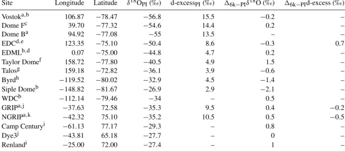
Table 1.Selected ice core records and their geographical coordinates, reported PI values ofδ¹⁸O and d-excess, and changes inδ¹⁸O and d-excess between 6k and PI. All values are given with respect to the V-SMOW scale.

Site Longitude Latitude δ¹⁸O_PI(‰) d-excess_PI(‰) 1_6k−PIδ¹⁸O (‰) 1_6k−PId-excess (‰)

Vostok^a,b 106.87 −78.47 −56.8 15.5 −0.2 –

Dome F^c 39.70 −77.32 −54.6 14.4 0.2 –

Dome B^a 94.92 −77.08 −55 13.5 – –

EDC^d,e 123.35 −75.10 −50.4 8.6 −0.3 0.7

EDML^b,d 0.07 −75.00 −44.8 4.7 0.2 –

Taylor Dome^f 158.72 −77.80 −40.5 4.9 1.5 –

Talos^g 159.18 −72.82 −36.1 3.9 −0.6 –

Byrd^h −119.52 −80.02 −32.9 4.5 −1.4 –

Siple Dome^b −148.82 −81.67 −26.9 2.9 −2.1 –

WDC^b −112.14 −79.46 −34 – 0.5 –

GRIP^a,j −37.63 72.58 −35.3 9.5 0.4 −0.2

NGRIP^a,k −42.32 75.10 −35.2 10.5 0.5 −0.5

Camp Centuryⁱ −61.13 77.17 −29.3 – 0.8 –

Dye3^j −43.81 65.18 −27.7 – 0 –

Renlandⁱ −25.00 72.00 −27.4 – 1 –

References:^areported in Risi et al. (2010b),^bWAIS Divide Project Members (2013),^cKawamura et al. (2007),^dStenni et al. (2010),^eLandais et al. (2015), fSteig et al. (2000),^gStenni et al. (2011),^hBlunier and Brook (2001),ⁱVinther et al. (2009),^jVinther et al. (2006),^kNorth Greenland Ice Core Project members (2004).

3 Results of the model–data comparison

3.1 Evaluation of MPI-ESM-wiso under PI conditions 3.1.1 Water isotopes in precipitation

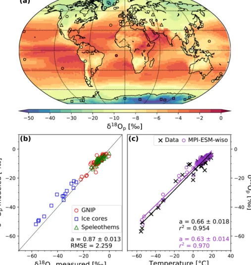
Figure 1a shows the global distribution of the simulated annual mean δ¹⁸Op values in precipitation. The main well- known patterns of the globalδ¹⁸O_pdistribution can be found in the model. They are very similar to those already observed with ECHAM5/MPIOM (Werner et al., 2016) and in agreement with present-day observations (circles: GNIP, squares:

ice cores, triangles: speleothems). Typically, enhanced¹⁸O- depleted precipitation with decreasing temperature (temperature effect) and increased altitude (altitude effect) is well simulated by MPI-ESM-wiso. The lowest simulated values of δ¹⁸O_p occur over the polar regions, with the minimum value over East Antarctica (−54.5 ‰). A decrease inδ¹⁸O_p is also observed going inland (continental effect) and with increased precipitation intensity over the low latitudes (precipitation amount effect).

In Fig. 1b, we compare our modeled δ¹⁸Opwith the observational dataset described in Sect. 2.3. The speleothem PI values ofδ¹⁸O_cin calcite are converted to δ¹⁸O_p in precipitation by using Eqs. (1) and (2). The modeled δ¹⁸O_p values are in very good agreement with the observations, with a linear regression gradient of 0.87 (1.0 being the per- fect fit) and a root mean square error (RMSE) of 2.3 ‰.

This represents an improvement compared to the modeled results from ECHAM5/MPIOM (RMSE of 3 ‰; Werner et al., 2016). The modeled globalδ¹⁸O_p–temperature relationship (for temperature below 20 ^◦C; Fig. 1c) is also improved

with a gradient 0.63 ‰^◦C⁻¹ (r²=0.97), very close to the observed one (0.66 ‰^◦C⁻¹,r²=0.95). This improvement, compared to the results from Werner et al. (2016), is mainly due to a better model–data agreement for the very low temperatures over the poles, which constitute an extreme test for isotope-enabled GCMs. This is confirmed by the good agreement of our modeledδ¹⁸Op–temperature spatial gradient over Antarctica (0.71 ‰^◦C⁻¹,r²=0.97) with the gradient of 0.8 ‰^◦C⁻¹ deduced from the Antarctic isotopic observations compiled by Masson-Delmotte et al. (2008).

However, even if the warm bias for the coldest temperatures over Antarctica is reduced, the modeledδ¹⁸O_pvalues are still too high at these locations (Fig. 1b). Concerning the δ¹⁸O_p–precipitation spatial gradient, we calculate observed and modeled values of−0.47 and−0.36 ‰ mm⁻¹d, respectively, for the nine low-latitude GNIP stations with an annual mean temperature equal or above 20^◦C. These results have to be taken with caution because of the few available tropical GNIP station records. The rather large standard errors of the gradients, estimated by using the variance–covariance matrix between the regression coefficients, illustrate this point well (0.165 and 0.145 ‰ mm⁻¹d for GNIP and MPI-ESM-wiso results, respectively).

3.1.2 Water isotopes in ocean surface waters

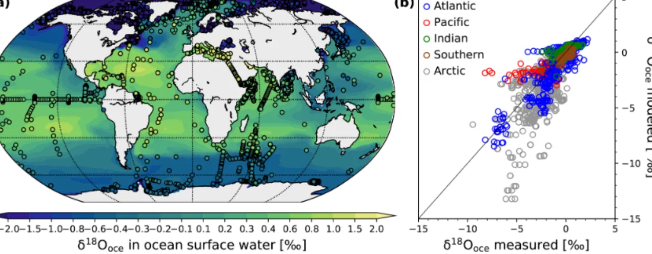
Figure 2a shows the global distribution of modeled annual meanδ¹⁸O_ocein ocean surface water (mean between 0 and 10 m of depth) and the comparison with the observations from the GISS database (colored dots). As expected from the data, we observe higher modeledδ¹⁸O_ocevalues in the low-

(8)

Figure 1.(a)Global distribution of simulated (background pattern) and observed (colored markers; see text for details) annual meanδ¹⁸O_p values in precipitation under PI conditions. The data consist of 70 GNIP stations (circles), 15 ice core records (squares; Table 1) and 33 speleothem records (triangles).(b) Modeled vs. observed annual meanδ¹⁸O_p at the different GNIP, speleothem and ice core sites.

(c) Observed (black crosses) and modeled (purple circles) spatialδ¹⁸Op–T relationship for the sites where the observed annual mean temperatures are below +20^◦C. The linear fits for the observed and modeled values are drawn as black and red lines, respectively. For both(b)and(c), the gradients of the linear regression fits are given in the legends.

latitude to midlatitude oceanic areas, which range between

−0.2 ‰ in the Malaysian area and 1.1 ‰ in the Bermuda area. The higher values in the Atlantic Ocean can be explained by a net freshwater export of Atlantic Ocean water, which is transported westwards to the Pacific (Broecker et al., 1990; Lohmann, 2003; Zaucker and Broecker, 1992).

Other highδ¹⁸O_ocevalues can be found in more localized areas like the Mediterranean Sea, the Red Sea, the Aden Gulf and the Persian Gulf, withδ¹⁸Oocevalues reaching+3.9 ‰ in the latter. The regional net freshwater export again ex- plains these increases inδ¹⁸Oocevalues. Contrary to Werner et al. (2016), who observed highδ¹⁸Oocevalues in the Black Sea, we obtain lowδ¹⁸Oocevalues between−1 and−2.7 ‰ in this small-scale area, which is in better agreement with the observations. This opposite result is due to the land–sea mask of higher resolution applied in our model (T63GR15

against T31GR30 used in Werner et al., 2016) that results in a narrower connection between the Black Sea and the Mediterranean Sea via the Aegean Sea. At high latitudes, the δ¹⁸O_ocevalues are lower than the average. In the Southern Ocean, the modeledδ¹⁸O_oce values are between −0.4 and

−1 ‰, in agreement with the observations. The most ¹⁸O- depleted ocean surface waters are in the Arctic Ocean, where theδ¹⁸O_ocevalues decrease down to−13 ‰. These very low δ¹⁸Oocevalues are mainly caused by highly¹⁸O-poor Arctic river discharges combined with a strong stratification of the simulated Arctic Ocean water masses (not shown).

In a similar way as for the atmospheric part, we compare our simulatedδ¹⁸Ooce values with the isotopic observations between 0 and 10 m of depth (GISS database; see Sect. 2.3) for a more quantitative evaluation of our model results (Fig. 2b). For the Atlantic Ocean (blue circles), the Pa-

(9)

cific Ocean (red circles), the Indian Ocean (green circles) and the Southern Ocean (brown circles), the model–data comparison does not show any systematic deviations between the modeledδ¹⁸O_ocevalues and the GISS data, characterized by RMSE values lower than 1 ‰ (Atlantic: r²=0.83, RMSE

=0.98 ‰; Pacific:r²=0.67, RMSE=0.68 ‰; Indian:r²= 0.48, RMSE=0.44 ‰ and Southern: r²=0.68, RMSE= 0.32 ‰). As already reported in Werner et al. (2016), the deviations from the observations are due to the overestimation of δ¹⁸O_oce values near river estuaries around the Amazon and the Sea of Okhotsk. For the Arctic Ocean, our simulated δ¹⁸Oocevalues are in better agreement with the observations (r²=0.57, RMSE=1.61 ‰) compared to the results from Werner et al. (2016) (r²=0.33, RMSE=2.25 ‰). However, our simulated δ values are still lower than the observations for many data entries. Because of the strong stratification of the simulated Arctic Ocean water masses, the highly ¹⁸O- depleted water inflows from Arctic rivers remain in the up- per layers of the Arctic Ocean without being well mixed with deeper waters.

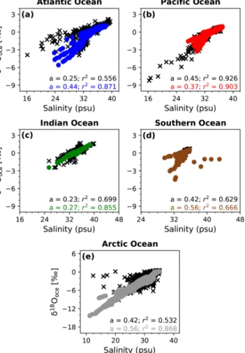
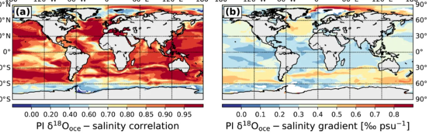
In Fig. 3, we analyze the relationship betweenδ¹⁸O_ocein ocean surface water and salinity for the Atlantic (Fig. 3a), Pa- cific (Fig. 3b), Indian (Fig. 3c), Southern (Fig. 3d) and Arc- tic Ocean (Fig. 3e). MPI-ESM-wiso is in fairly good agreement with the observations in terms of absolute values and δ¹⁸O_oce–salinity gradients, the latter varying between 0.27 and 0.56 ‰ psu⁻¹. The best agreements with the observations are in the Indian and the Pacific Ocean, even if the model is not able to reach the lowest δ¹⁸Ooce and salinity values around the Sea of Okhotsk and the Bering Sea. Ex- cept for the Pacific Ocean, the relationship betweenδ¹⁸Ooce

and salinity in the different basins, expressed by the correlation coefficients r², is stronger in the model (0.87, 0.90, 0.86, 0.67 and 0.87 for the Atlantic, Pacific, Indian, South- ern and Arctic Ocean, respectively) than in the observations (0.56, 0.93, 0.70, 0.63 and 0.53, respectively). The main disagreement in the deducedδ¹⁸O_oce–salinity gradient is in the Atlantic Ocean, with a steeper gradient in MPI-ESM-wiso than in the GISS data. The latter is due to the underestimation by the model of theδ¹⁸O_ocevalues in the northwest At- lantic along the Canadian coast (Fig. 2). ¹⁸O-depleted water inflows from Canadian rivers and the strong ocean dynamics of this area with important interconnected currents, probably not well constrained by MPI-ESM-wiso, can ex- plain the model–data mismatch. In the Arctic and Southern Ocean, even if the modeledδ¹⁸Ooce–salinity gradient is similar to the observed one, the model underestimates both the δ¹⁸O_oce and salinity values, probably because of the major roles played by river discharges and changes in sea ice in these areas.

3.1.3 Deuterium excess

The modeling of the deuterium-excess signal is challenging for GCMs. For the North Atlantic and Arctic Ocean region,

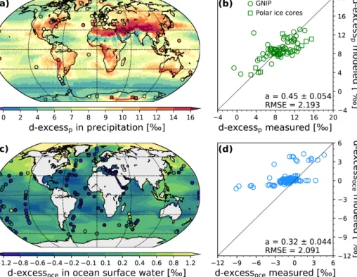
the spatial structure of the marine boundary layer water vapor isotopic composition, which greatly influences the d-excess signal in precipitation, seems to be poorly simulated by the models (Steen-Larsen et al., 2017). Model deficits might be linked to sublimation and moisture source processes over sea-ice-covered areas (Bonne et al., 2019; Klein and Welker, 2016). Moreover, in higher latitudes, the representation of d- excess is very sensitive to supersaturation in polar clouds, which is a poorly constrained empirical parameter (Jouzel and Merlivat, 1984; Risi et al., 2013). A comparison of our simulated d-excess signals with available data thus represents a good evaluation test for our model. Figure 4 shows the simulated deuterium excess in precipitation (d-excessp) and ocean surface water (d-excessoce). The modeled values of d-excessp (Fig. 4a) range between 0 ‰ and 20 ‰. The highest values are in the northern part of the Sahara and in a 25–45^◦N band going from Saudi Arabia to the Himalaya.

The lowest values are found in dry regions like the southern Sahara between the latitudes 25 and 10^◦N, Oman and Rajasthan (India), and over the Southern Ocean (between 2 and 6 ‰), which is an area with large net freshwater input (P−E). For the Antarctic continent, the contrast between the low values of d-excess_pin the west and high values in the east is well captured by the model, in agreement with the observations. The quantitative model–data comparison (Fig. 4b) shows that the modeled d-excess_pvalues are in fairly good agreement with the observations. However, MPI-ESM-wiso tends to underestimate the d-excesspvalues, especially where the observations are higher than 8 ‰.

The modeled d-excessocevalues (Fig. 4c) range between

−8 ‰ (Persian Gulf) and +7 ‰ (Baltic Sea). We can dis- tinguish between the middle to low latitudinal region of the Atlantic Ocean with lower d-excess_ocevalues (between−0.2 and−0.8 ‰), the Arctic Ocean where modeled d-excess_oce values vary from 0 ‰ in the north of the Atlantic Ocean to +7 ‰ along the northern coast of Siberia, and the remaining ocean surface waters with smoother variations in their d-excess_ocevalues (from−0.2 to 0.6 ‰). The negative d-excess_oce signal in the middle to low latitudinal Atlantic Ocean is due to the presence of a net freshwater export. As the exported water masses and the evaporation have a positive deuterium-excess value, the d-excessocein the remaining water becomes more negative due to the hydrological balance. This is the opposite for areas with positive d-excessoce

values, like in the Baltic Sea and the Arctic Ocean, where there is a surplus of precipitation (positiveP−E) with positive deuterium-excess values. The quantitative comparison with the GISS database (Fig. 4d) shows that MPI-ESM-wiso globally overestimates the deuterium-excess values in ocean surface water. The model is especially not able to reach the very low values observed in the Mediterranean Sea and overestimates the d-excess_oce values in the Baltic Sea. Potential model–data mismatches can be due to different vertical layer thicknesses, which influence the surface kinetic fractionation. The horizontal model resolution, which is too coarse,

(10)

Figure 2.(a)Comparison of the global distribution of simulated (background pattern) annual meanδ¹⁸Oocevalues in ocean surface water (mean over the first 10 m of depth) under PI conditions with observedδ¹⁸O_ocevalues of the GISS database (colored dots).(b)Scatter plot of observed vs. modeledδ¹⁸Oocevalues for the Atlantic (blue circles), Pacific (red circles), Indian (green circles), Southern (brown circles) and Arctic Ocean (grey circles). The month of sampling has been considered for this scatter plot.

can also affect the model–data comparison on a global scale, especially where strong small-scale variations in observed d- excess_oceare found.

MPI-ESM-wiso overestimates the deuterium excess in the ocean surface and underestimates the deuterium excess in precipitation, especially for the highest observed values.

However, the modeled linear relationship between the deuterium excess in water vapor above the ocean surface (d- excessvap) and the near-surface relative humidity (RH, expressed between 0 and 1) is d-excess_vap=50.12−52.81× RH, in very good agreement with the equation given by Pfahl and Sodemann (2014). One possible explanation for the positive and negative biases of modeled d-excess concentrations in the ocean surface water and precipitation, respectively, could be the description of fractionation processes during the evaporation of ocean surface water taken from Merli- vat and Jouzel (1979), which would distribute too much d- excess in ocean surface water and not enough in the water vapor (and so in the precipitation). This agrees with the studies from Steen-Larsen et al. (2014a, b, 2015); Steen-Larsen et al. (2017) and Bonne et al. (2019), which show biases in the simulated deuterium-excess signal in water vapor in Greenland, the North Atlantic and the Arctic Ocean in several GCMs compared to in situ measurements of surface water vapor isotopes.

3.2 Mid-Holocene simulation

3.2.1 Changes in near-surface air temperature and precipitation

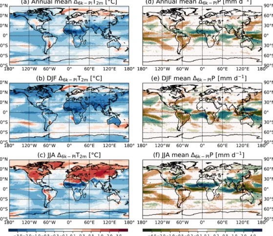
Before analyzing the 6k isotopic anomalies, we check that our modeled 6k−PI anomalies in standard climate variables, like the 2 m temperature and the precipitation rate, are consistent with previous studies. For that, we show in Fig. 5

the simulated annual mean boreal winter (DJF) and summer (JJA) changes in the 2 m temperature and precipitation rate between the 6k and PI climates. Because of the different values in orbital parameters and greenhouse gases, the mid- Holocene is characterized by a slightly colder mean global climate compared to the modeled PI (−0.42^◦C). The simulated anomalies in annual mean temperature are rather small, with 6k−PI changes of less than 1^◦C (Fig. 5a) in most regions. The exception is the Saharan area where a cooling in the range of−1 to−4^◦C can be observed due to the enhanced African monsoon. We also observe a slight increase in annual mean temperature over the western Arctic area, northern Siberia and eastern Europe. As a first result, we conclude that the 6k−PI anomalies in annual mean temperature from MPI-ESM-wiso are globally consistent with the PMIP2 and CMIP5/PMIP3 model results (Harrison et al., 2014). The annual mean change in precipitation amount is very small (less than 1 mm yr⁻¹), in agreement with the previous PMIP2 and CMIP5/PMIP3 model results (Harrison et al., 2014). The African (20^◦W–30^◦E, 10–20^◦N region) and Indian (70–100^◦E, 20–40^◦N region) monsoons are enhanced during mid-Holocene by+1.06 and+0.37 mm d⁻¹, respectively (Fig. 5d), consistent with the PMIP3 results (https://pmip3.lsce.ipsl.fr, last access: 20 September 2019).

The changes in orbital forcing lead to a northward expan- sion of the African monsoon. This is also in agreement with previous coupled model results (Braconnot et al., 2007; Har- rison et al., 2014), even if this monsoon extension is still not large enough compared to the observations (Perez-Sanz et al., 2014).

One of the characteristics of the 6k climate is the enhanced seasonal contrast in the Northern Hemisphere due to changes in the insolation, giving rise to warmer North- ern Hemisphere summers (Fig. 5c). There is a strong land–

(11)

Figure 3.Scatter plots ofδ¹⁸O in ocean surface water vs. surface salinity for the(a)Atlantic,(b)Pacific,(c)Indian,(d)Southern and (e)Arctic Ocean under PI conditions. The black crosses correspond to the data from the GISS database and the colored dots to the modeled values. The gradients and the correlation coefficients of the linear regression fits are given in the legends.

ocean contrast, with the main positive temperature anomalies on land. They range between +0.5 and +3^◦C, the highest values being over North America and Mongolia, while the 6k−PI summer temperature anomalies in middle and high latitudes over the ocean and the Arctic are lower than 0.5^◦C, except near the Greenland coasts. In lower Northern Hemi- sphere latitudes, the summer surface temperature anomalies over the ocean are generally lower (between 0 and−1^◦C).

In the Southern Hemisphere, positive mean JJA temperature anomalies (i.e., austral winter) can be observed over South America, Australia and coastal West Antarctica. The mean 6k JJA temperature anomalies over the ocean are globally lower, except for some locations in the Southern Ocean near the Antarctic coast. All these results are consistent with the previous PMIP simulations (Braconnot et al., 2007; Harrison et al., 2014). The colder 6k boreal summer in the region from West Africa to India is the consequence of increased precipitation linked to the monsoon changes (Fig. 5f) over this area

(Braconnot et al., 2007). The positive anomalies in precipitation over Africa and India are the strongest during the boreal summer, with mean values of+2.42 and+1.00 mm d⁻¹, respectively. We also find a dipole in the response of the monsoons over the Pacific–Indian area, with enhanced rainfall in the Equator sector of the Indian Ocean and reduced rainfall over the Indonesian region. For the mean DJF temperatures (Fig. 5b), we find negative anomalies over the Antarctic continent and positive anomalies over the surrounding Southern Ocean (between 0 and 0.5^◦C). Over the rest of the globe, the 6k−PI anomalies in mean DJF surface temperatures are generally negative.

3.2.2 6k changes inδ¹⁸Osignals

Even if the changes in temperature and precipitation amount are modest compared to periods like the LGM, they leave imprints on δ¹⁸O_p in precipitation values (Fig. 6a). MPI- ESM-wiso simulates a precipitation-weighted mean global decrease inδ¹⁸O_pby−0.16 ‰, which is in good agreement with the model results from LeGrande and Schmidt (2009).

Positive simulated 6k−PIδ¹⁸O_pchanges, ranging from+0.3 to+1 ‰, are found over the Arctic area including Greenland, Alaska and the northern part of Siberia. They are likely associated with higher summer temperatures and reductions in Arctic sea ice during 6k (LeGrande and Schmidt, 2009). For the distribution ofδ¹⁸Opanomalies over Antarctica, three areas can be distinguished: one region from the 180th meridian to 90^◦W with anomalies slightly negative or close to zero, another area from 90^◦W to 100^◦E with positive anomalies of δ¹⁸Op, and the remaining region between 100 and 180^◦E with negative isotopic anomalies. Except for Aus- tralia, the Indonesian area and some coastal regions in the American continent, negative 6k−PI changes occur in general over the remaining land surfaces. The strongest negative anomalies (−5.43 ‰) are located over the southern Sa- hara where a strong decrease in surface temperature and amplified African monsoon are simulated by MPI-ESM-wiso.

Strong negative changes inδ¹⁸O_palso occur over the Tibetan Plateau, with values ranging from−0.5 to−3.5 ‰. This is probably due to the lower simulated values of annual mean temperature in this area during the 6k period combined with an enhanced precipitation rate, especially in summer (Fig. 5).

Finally, MPI-ESM-wiso simulates positive 6k−PI anomalies of δ¹⁸Op between +0.2 and +1 ‰ in the western Pacific Ocean and over the Indonesian area linked to lower rainfall during mid-Holocene.

Next, we compare our simulated 6k−PIδ¹⁸O_panomalies with isotopic observations from the ice cores and speleothem records described in Sect. 2.3 (Fig. 6b). In general, our modeled isotopic anomalies are in fair agreement with the data (r²=0.38 and RMSE =0.79 ‰). The modeled posi- tiveδ¹⁸O_panomalies over most parts of Greenland are confirmed by the polar ice core measurements and the negative anomalies over the southern Greenland coast. The

(12)

Figure 4.Global distribution of simulated and observed annual mean d-excess values in precipitation(a)and ocean surface waters(c).

Scatter plots of modeled vs. observed annual mean deuterium-excess values in precipitation(b)and ocean surface waters(d)are shown. The gradients and RMSE of the linear regression fits are given in the legend.

largest deviation is found for the coastal Renland ice core (1_6k−PIδ¹⁸O_p= +1 ‰) for which MPI-ESM-wiso simulates aδ¹⁸O_panomaly of+0.25 ‰, which is too low. The modeled positive–negative contrast in the1_6k−PIδ¹⁸O_pdistribu- tion between the central and eastern parts of Antarctica is also found in the data (EDC, Vostok and Talos ice cores in the east; Dome Fuji and EDML in the central area). How- ever, there is a disagreement in the west of the continent, with modeledδ¹⁸O_panomalies close to zero, while the observations are clearly positive (WDC ice core) or negative (Byrd and Siple Dome ice cores). In the most eastern region of Antarctica (160^◦E), near the Ross Sea, MPI-ESM- wiso is not able to catch the positive 6k−PIδ¹⁸Opanomaly at the Taylor Dome site. Concerning the δ¹⁸O anomalies from calcite in speleothems, all our simulated 6k−PI isotopic changes are of the same sign as the speleothem data if we include an uncertainty of ±0.5 ‰, as in Comas-Bru et al. (2019). The model reproduces the observed negative and positive 6k−PI changes inδ¹⁸O_cwell over the Tibetan Plateau and the coastal areas of the South American continent, respectively. Disagreements with the speleothem data are found in the US and in Europe where observed positive anomalies are not captured by MPI-ESM-wiso. The largest deviations are found for two speleothems located in Ethiopia (16k−PIδ¹⁸Omodel= −0.59 ‰ and16k−PIδ¹⁸Oreconstructed=

−3.31 ‰) and in the Great Basin of western North America (16k−PIδ¹⁸Omodel= −0.28 ‰ and16k−PIδ¹⁸Oreconstructed=

+1.36 ‰). These discrepancies likely reflect an insufficient amplification of the precipitation rate (or its wrong location) over eastern Africa and an increase in temperature that is too weak over northeast America during the mid-Holocene period. More generally, the amplitude of the modeledδ¹⁸O changes at speleothem sites is underestimated by MPI-ESM- wiso. This is likely related to the underestimation by the model of the 6k changes in climate variables like the temperature and precipitation rate, as already noticed in previous model studies (Harrison et al., 2014).

Concerning the changes in d-excessp in precipitation, we find negative anomalies over Antarctica and Greenland. The modeled d-excessp value at the EDC site is of opposite sign compared to the measured value (1_6k−PId-excess_model= −0.45 ‰ and 1_6k−PId-excess_obs= +0.7 ‰), while the Greenland values are consistent with the observations (GRIP:

1_6k−PId-excess_model= −0.28 ‰ and 1_6k−PId-excess_obs=

−0.2 ‰; NGRIP: 1_6k−PId-excess_model= −0.20 ‰ and 1_6k−PId-excess_obs= −0.5 ‰).

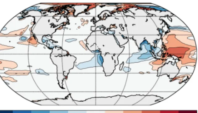
Figure 7 shows our modeled annual mean changes in δ¹⁸O_ocein ocean surface water between 6k and PI. The simulated annual meanδ¹⁸O_ocechange between 6k and PI is very small (−0.01 ‰), in agreement with previous model results (LeGrande and Schmidt, 2009). The model simulates an increase in δ¹⁸Ooce in the Arctic Ocean ranging from 0.1 to 0.7 ‰, except around the 180th meridian, which is related

(13)

Figure 5.Simulated annual, boreal winter (DJF) and boreal summer (JJA) changes in 2 m temperature(a, b, c)and precipitation(d, e, f) between 6k and PI.

to Arctic sea ice reductions and warmer summers in 6k relative to PI. Higherδ¹⁸O_pvalues in precipitation are observed, too. Enhanced runoff with lowerδ¹⁸O values (not shown) is associated with negative 6k−PI anomalies inδ¹⁸O_ocealong the coasts of central America and southwestern Africa, the Red Sea, the Persian Gulf, and the Bay of Bengal. As for the changes inδ¹⁸O_p, MPI-ESM-wiso simulates a dipole of higher–lowerδ¹⁸Oocevalues compared to the PI state in the western Pacific Ocean (from +0.05 ‰ to+0.5 ‰) and the Bay of Bengal (from−0.05 ‰ to−1 ‰), respectively. Pos- itiveδ¹⁸Ooce changes are also found in the subtropical latitudes of the eastern Pacific Ocean. The increase inδ¹⁸Ooce

values during 6k relative to PI is due to the lower annual mean precipitation rates over these areas and vice versa.

Slight positive δ¹⁸O_oce anomalies are also simulated along the western Antarctic coast related to the higher 6k summer temperatures over the Southern Ocean.

4 Temporal relationships between the water isotopes and climate variables

The classical use of water isotopes to reconstruct past variations of climate implies that the modern spatial relationship

between isotopes and climate variables, such as surface temperature, precipitation rate and salinity, can be taken as a sur- rogate for the temporal isotope–climate gradient at a given site. Such temporal relationships can be calculated from our model results. In Sect. 4.1, we first look at the interannual variability between water isotopes and 2 m temperature, precipitation rate and salinity under PI conditions. We limit the analysis to the interannual gradients from our PI simulation as they are qualitatively similar to the ones derived from our 6k simulation. The corresponding figures for the 6k period (Figs. S1 and S3) and their differences from PI results (Figs. S2 and S4) are in the Supplement. Then, we examine the long-term temporal 6k−PIδ¹⁸O gradients versus the different climate variables in Sect. 4.2.

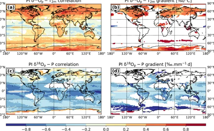
4.1 Interannual relationships of water isotopes and climate variables for the PI climate

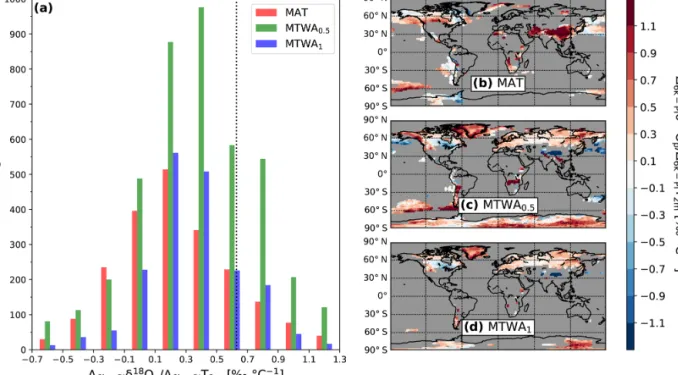
In the same way as previous studies (Schmidt et al., 2007;

Risi et al., 2010b; Roche and Caley, 2013), we calculate for each grid box the interannual relationship (correlation coefficients and gradients) between monthly anomalies ofδ¹⁸O_p and temperature and precipitation rate over the 150 years of our PI simulation. These monthly anomalies are calculated