Observed and modeled biogeochemistry of ﬁlaments oﬀ Peru

(1)

Observed and modeled biogeochemistry of filaments off Peru

A thesis submitted in fulfillment of the requirements for the degree:

Master of Science

Climate Physics: Meteorology and Physical Oceanography

Faculty of Mathematics and Natural Sciences Christian-Albrechts-Universität zu Kiel

Kiel, December 2017

Author: Jaard-Okke Frederik Hauschildt Matrikel-Nr. 5657

1. Advisor: Prof. Dr. Andreas Oschlies 2. Advisor: Dr. Sören Thomsen

(2)

(3)

Abstract

The biogeochemistry of an observed cold filament off Peru and the representation of filaments in submesoscale-permitting (1/45^◦) coupled biogeochemical model simulations are the focus of this thesis. Furthermore, we use the simulations to investigate the effect of submesoscale frontal processes on the distribution of biogeochemical tracers in the shallow oxygen minimum zone off Peru. The observed filament contains relatively cold, fresh and nutrient-rich waters originating in the coastal upwelling. Enhanced nitrate concentrations and offshore velocities of up to 0.5 m s⁻¹ within the filament suggest an offshore transport of nutrients. Despite low chlorophyll α concentrations in the core of the filament, depth integrated primary production is 40% higher than at the upwelling front and 25%

higher than offshore. The highly variable relationship of surface chlorophyll α and depth- integrated primary production highlights the inherent uncertainty of primary production estimates based on ocean-color measured by satellites. The observations are used to assess the results of two different biogeochemical model simulations (PISCES / BioEBUS). Both simulations exhibit filaments that are similar in lateral scale, horizontal and vertical structure and offshore extent to those observed, but differences exist in the biogeochemistry:

While the PISCES simulation exhibits nitrate concentrations within filaments comparable to observations, filaments are largely depleted of nitrate in the BioEBUS simulation. This difference can be related to a higher pyhtoplankton growth rate and faster nitrate uptake in BioEBUS. The importance of sufficiently slow phytoplankton growth for maintaining realistic concentrations of upwelled nutrients offshore is therefore stressed. Furthermore, the simulations suggest that submesoscale frontal processes increase subduction and offshore export of nitrate which leads to reduced primary production. An increase in oxygen that resembles the pattern of the decrease in nitrate suggests a ventilation of the shallow oxygen minimum zone off Peru by vertical and horizontal eddy-fluxes.

(4)

Die Biogeochemie eines beobachteten Kaltwasserfilaments vor Peru und die Darstellung von Filamenten in gekoppelten biogeochemischen Modellsimulationen die Teile des submesoskaligen Regimes explizit auflösen (1/45^◦) sind der Fokus dieser Masterarbeit. Zusät- zlich verwenden wir die Simulationen, um den Effekt von submesoskaligen Frontenprozessen auf biogeochemische Tracerverteilungen in der oberflächennahen Sauerstoffminimumzone vor Peru zu untersuchen. Das beobachtete Filament enthält relativ kaltes, frisches und nährstoffreiches Wasser, das dem küstennahen Auftriebsgebiet entstammt. Erhöhte Ni- tratkonzentrationen und seewärtige Strömungsgeschwindigkeiten von bis zu 0.5 m s⁻¹ innerhalb des Filaments deuten auf einen seewärtigen Transport von Nitrat hin. Trotz niedriger Chlorophyll α Konzentrationen im Kern des Filaments ist die über die Tiefe integrierte Primärproduktion um 40% höher als an der Auftriebsfront und um 25% höher als im offenen Ozean. Die sehr variable Beziehung von Chlorophyll α an der Oberfläche und der über die Tiefe integrierten Primärproduktion zeigt die Unsicherheit auf, die mit Schätzungen der Primärproduktion auf Basis von Satellitenmessungen verbunden ist. Die Beobachtungen werden benutzt um zwei unterschiedliche biogeochemische Modellsimula- tionen (PISCES / BioEBUS) zu bewerten. Beide Simulationen zeigen Filamente die den beobachteten in der seitlichen und der seewärtigen Ausdehnung sowie in der horizontalen und vertikalten Struktur ähneln, aber es existieren Unterschiede in der Biogeochemie:

Während die PISCES Simulation mit Beobachtungen vergleichbare Nitratkonzentrationen innerhalb von Filamenten zeigt, ist das Nitrat in Filamenten in der BioEBUS Simulation gröstenteils aufgebraucht. Dieser Unterschied kann mit einer höheren Wachstumsrate von Phytoplankton und damit schnellerer Nitrataufnahme in BioEBUS in Verbindung gebracht werden. Die Bedeutung von ausreichend langsamem Phytoplankton-Wachstum für das Aufrechterhalten realistischer Konzentrationen von aufgetriebenen Nährstoffen im offenen Ozean wird daher betont. Weiterhin deuten die Simulationen darauf hin, dass submesoskalige Frontenprozesse die Subduktion und den Export von Nitrat in den of-

(5)

fenen Ozean erhöhen, was zu verringerter Primärproduktion führt. Eine Zunahme von Sauerstoff die dem Muster der Abnahme von Nitrat ähnelt deutet auf eine Ventilation der oberflächennahen Sauerstoffminimumzone vor Peru durch vertikale und horizontale Wirbelflüsse hin.

(6)

(7)

1 Introduction

The eastern margins of the subtropical oceans are characterized by upwelling of cold and nutrient-rich subsurface waters, caused by persistent along-shore winds that drive an offshore Ekman transport. The nutrients supplied to the sunlit surface ocean subsequently fuel high phytoplankton growth which supports a rich ecosystem (Pennington et al., 2006).

These Eastern Boundary Upwelling Systems (EBUS) are found in all major ocean basins and named after the Canary, Benguela, California, and Peru-Chile current systems. The Peru-Chile upwelling system (PCUS) is the most productive EBUS in the world ocean accounting for 10 % of the global fishery production while occupying only 0.1 % of the ocean surface (Chavez et al., 2008). Furthermore, the high productivity and export of organic matter from the euphotic zone and its subsequent remineralization at depth by oxygen-consuming organisms lead to - in conjunction with poor ventilation by sluggish currents - the presence of the shallowest and most intense oxygen minimum zone (OMZ) in the world ocean which in turn affects marine life (Wyrtki, 1962;Paulmier et al., 2006;

Karstensen et al., 2008; Stramma et al., 2010). Because of the shallow oxycline that varies between only 10 m - 80 m depth and is often around 30 m (Hamersley et al., 2007), submesoscale frontal processes could potentially be important for its ventilation. The Peru upwelling ecosystem and the fisheries that depend on it thus have immense economical importance for the local population. Global relevance is given to EBUS by their role as natural sources of climate relevant trace gases to the atmosphere such as N₂O (Friederich et al., 2008; Arévalo-Martínez et al., 2015) and CO₂ (Chavez et al., 2007; Gruber, 2015).

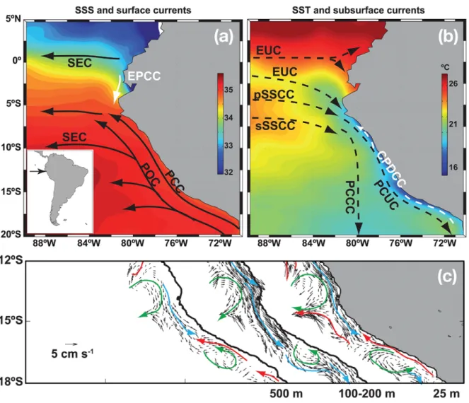
Two main along-shore currents off Peru are relevant for this study (Fig. 1): At the subsurface, the Peru-Chile Undercurrent flows poleward with a velocity of 10 - 15 cm s⁻¹ at 100 m - 150 m depth along the shelf (Wyrtki, 1963, 1967;Brink, 1983; Huyer et al., 1991;

Strub et al., 1998;Penven et al., 2005;Colas et al., 2012;Chaigneau et al., 2013). At the surface the Peru Coastal Current flows equatorward (Penven et al., 2005), but not continuously: Between 11^◦S - 16^◦S, southward surface velocities of 10 - 15 cm s⁻¹ are observed, related to a near-surfacing of the PCUC (Chaigneau et al., 2013). At 14^◦S a persistent eddy-like feature is observed, which results in mean offshore velocities at this latitude

(10)

Figure 1: (a) Sea-surface salinity and surface circulation. (b) Sea-surface temperature and subsurface circulation. Relevant currents for this study are the Peru Coastal Current (PCC) at the surface and the Peru-Chile Undercurrent (PCUC) (c) Mean current along the coast of Peru at 25 m, between 100 m and 200 m, and at 500 m depth.

Red and blue arrows represent the equatorward and poleward flows. Green arrows indicate mesoscale cyclonic (14^◦S) and anticyclonic (17^◦S) features. Figures taken from Chaigneau et al.(2013).

(11)

(Fig. 1c).

Mesoscale eddies, upwelling filaments and strong sea-surface temperature (SST) gradients at the upwelling front separating cold coastal from warm offshore waters are ubiquitous features in the PCUS (Penven et al., 2005; Colas et al., 2012; Thomsen et al., 2016a,b).

When the upwelling front meanders and eventually becomes unstable, an ageostrophic secondary circulation develops in order to restore geostrophic balance (Thomas et al., 2008; Mcwilliams et al., 2009;McWilliams et al., 2015). This ageostrophic flow field can drive large vertical velocities and thus impact the physical-biogeochemical coupling by modifying vertical and lateral transports of nutrients and organic matter (Lapeyre and Klein, 2006; Lévy et al., 2012; Mahadevan, 2015). Furthermore, frontal processes may provide an effective conduit for vertical fluxes of heat and gas between the subsurface ocean and the atmosphere (Ferrari, 2011;D’Asaro et al., 2011). While the submesoscale comprises of filaments, fronts, mixed-layer instabilities and symmetric instabilities, we focus here on filaments and fronts which constitute the upper end of the submesoscale variability spectrum with length scales of O(1 - 10) km.

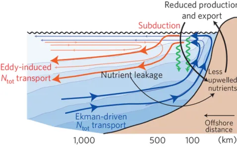
Eddies have in the past been assumed to generally enhance biological productivity by either exposing nutrient-rich subsurface water to the well-lit euphotic zone or by lateral advection of nutrients. They are considered a major source of nutrients to the oligotrophic subtropical gyres, although the magnitude of this supply and the processes involved have been discussed controversially (Falkowski et al., 1991; Oschlies and Garçon, 1998; Os- chlies, 2001, 2002; McGillicuddy et al., 1998, 2003, 2007; Mahadevan et al., 2008; Branni- gan, 2016). It has since become clear that the eddy-flux of any tracer strongly depends on the standing stock and its lateral and vertical gradients. In the highly productive EBUS, eddies and filaments have been shown to decrease productivity by exporting nutrients and organic matter offshore and downward below the euphotic zone (Rossi et al., 2008, 2009; Lévy, 2003;Lathuilière et al., 2010;Gruber et al., 2011; Nagai, 2015) as illustrated in Figure 2.

However, all of these studies are purely based on models and the quantification of submesoscale eddy-fluxes from observations has proven difficult. Submesoscale frontal processes

(12)

Figure 2: Conceptual diagram of the impact of mesoscale eddies on coastal circulation, nitrogen transport, and organic matter production and export. Figure taken from Gruber et al. (2011).

are intermittent and occur on small temporal scales of O(days) and horizontal scales of O(1 - 10 km), making them inherently difficult to observe. In order to capture these processes synoptically and separate temporal from spatial variability, towed underway systems (Pollard and Regier, 1992; Rudnick and Luyten, 1996;Thomas et al., 2013;Hosegood et al., 2017) or multiplatform adaptive sampling approaches using glider fleets (Thomsen et al., 2016a) are increasingly being used for high-resolution hydrographic measurements.

Horizontal currents can be measured by vessel-mounted acoustic doppler current profiler (ADCP), but vessel draft and ADCP blanking distance of around 20 m combined often exceed the mixed-layer depth (MLD) and thus do not capture the surface boundary layer where the strongest submesoscale flows are expected. Furthermore, the vertical velocities that characterize frontal processes and determine the associated vertical tracer fluxes can at present not be measured by ADCP at all, a deficit that some studies have overcome using acoustically-tracked neutrally buoyant floats providing Lagrangian estimates of the vertical velocity (Vélez-Belchí and Tintoré, 2001; D’Asaro et al., 2011). Satellite images allow for an identification of SST fronts, but satellite altimetry is limited to mesoscale

(13)

geostrophic current estimates that do not reveal the complex ageostrophic velocity structure associated with them. Observing submesoscale flows and their temporal variability thus remains challenging and technical as well as practical limitations preclude the quantification of submesoscale eddy-fluxes based on observations alone for the foreseeable future.

Here we conducted an integrated study in an attempt to close the gap between observations and models. We combine targeted shipboard observations of a cold filament and submesoscale-permitting coupled biogeochemical model simulations to address two main questions:

1. How does the observed biogeochemistry of cold filaments off Peru compare with their representation in submesoscale-permitting biogeochemical model simulations?

2. What is the role of filaments for primary production and the export of nutrients and oxygen into the shallow OMZ off Peru?

This thesis is structured as follows: First, an overview of historical measurements in the upwelling near 15^◦S off Peru is presented (Sec. 2), after which the filament survey that was carried out in this study is described (Sec. 3). A description of the coupled physical-biogeochemical model is given in section 4 along with an assessment of the impact of horizontal resolution on the simulations (Sec. 4.3) and differences between the two biogeochemical models (Sec. 4.4). An observed cold filament is characterized in section 5 and compared with the representation of filaments in biogeochemical model simulations in section 6, followed by a synthesis of observed and modeled filament characteristics that concludes the results (Sec. 6.3). The relevance of our results with respect to the questions above and in the context of the existing literature is discussed in section 7. A summary of this thesis and an outlook on future work and possible improvements of the model simulations is given in section 8.

(14)

2 Historical measurements in the upwelling off Peru

The coldest and most persistent upwelling in the PCUS is located near 15^◦S off Pisco (Zuta and Urquizo, 1972). Several studies have focused on this persistent upwelling in the past using integrated physical and biogeochemical, shipboard and airborne observations carried out off the coast of Peru during the years 1966, 1969, 1976 and 1977 (Armstrong et al., 1967; Minas et al., 1974; Walsh et al., 1971; Dagg et al., 1980; Brink et al., 1981;

Nelson et al., 1981;Brink, 1983;Boyd and Smith, 1983;Smith, 1983;Packard et al., 1983;

Dengler, 1985;Macisaac et al., 1985). Even though these studies were conducted at a time well before satellite measurements and digital communication were ubiquitous, adaptive sampling strategies were implemented with a technical effort that is still impressive 30 - 50 years later. Macisaac et al.(1985) acquired biogeochemical measurements in a lagrangian framework following surface drogues. They planned their measurements according to sea- surface temperature with the support of an aircraft that mapped the area every other day and delivered maps of the previous day’s temperature field to the ship by air drop.

Underway measurements by autoanalyzer of nitrate, nitrite, ammonium, phosphate and silicate with a horizontal resolution of 250 m were carried out by Dengler (1985).

Cold water plumes extending offshore from the upwelling patch at distinct topographic features of the coastline, with an offshore extent related to the observed wind speed were also described by most of the early studies in underway measurements and infrared images taken by aircraft, features that would some years later be termed upwelling filaments (Flament and Washburn, 1985). Also consistently described are low phytoplankton concentrations within ~ 20 km from the coast despite an abundance of nitrate in the recently upwelled water, a feature that is also observed in satellite images during our survey (Fig. 12b). Three factors were proposed over the years to contribute to these high-nutrient, low-chlorophyll (HNLC) conditions in the upwelling center and generally in the eastern tropical Pacific, which will be outlined in the following: (1) A time lag of phytoplankton growth after upwelling (Armstrong et al., 1967; Boyd and Smith, 1983; Macisaac et al., 1985), (2) grazing pressure by herbivorous zooplankton (Minas et al., 1974; Walsh, 1976;

Whitledge, 1981) and (3) nutrient limitation of phytoplankton growth by a lack of sil-

(15)

ica (Nelson et al., 1981) or iron (Hutchins et al., 2002; Bruland et al., 2005). Macisaac et al. (1985) investigated the timescale of phytoplankton growth in the upwelling center near 15^◦S in a lagrangian framework and found that the time required to complete a full growth cycle of upwelling, increase of nutrient uptake and finally nutrient depletion was 8 - 10 days. The growth cycle in their study is completed in the near-shore upwelling and maximum nutrient uptake already occurs at 10 km from the coast, indicating that the phytoplankton growth timescale cannot explain HNLC conditions further offshore. However, the trajectories of their drogues show a large along-shore component of the flow, suggesting that the HNLC area that is influenced by the phytoplankton growth timescale may be larger in conditions where a stronger offshore flow is present. Minas et al. (1974) first suggested that grazing by herbivorous zooplankton immediately after upwelling keeps the phytoplankton concentrations low, thereby slowing down the initial phytoplankton growth and reducing nutrient uptake which is an effective way to spread upwelled nutrients to the open ocean. The slowly growing phytoplankton standing stock observed in the PCUS was explained by a higher abundance of zooplankton in the euphotic zone due to the suboxic waters below and thus higher grazing pressure. This grazing hypothesis (Walsh, 1976) was the generally accepted explanation for the occurrence of HNLC conditions until it was discovered that a lack of iron can limit phytoplankton growth in the PCUS upwelling system (Hutchins et al., 2002;Bruland et al., 2005). Given the many possible explanations for HNLC conditions, Pennington et al. (2006) in their review of primary production in the Pacific arrive at the conclusion that not a single but multiple interdependent processes - mainly iron limitation and grazing - are likely responsible for the observed low Chlα concentrations. A possible interaction between different processes would be that iron limitation favors small phytoplankton which may be more susceptible to zooplankton grazing pressure which then limits the growth rate. A recent modeling study by Vergara et al. (2017) revisited the question of nutrient limitation of phytoplankton growth in the PCUS and found that iron is the limiting nutrient in winter and a co-limitation of silica and nitrate exists in summer. Dengler (1985) found both nitrate and silica to be above limiting levels in the PCUS during a survey in April - June 1976.

(16)

This brief literature review shows that HNLC conditions are ubiquitous in the PCUS and that the generating mechanisms are - although complex and still not fully understood - likely a combination of multiple interdependent biogeochemical processes. Furthermore, the timescale of phytoplankton growth following upwelling can be expected to impact the amount of nitrate and carbon that is subducted by filaments. Given a slowly growing phytoplankton standing stock, upwelled nutrients can be subducted below the euphotic zone before they are taken up by phytoplankton. It is therefore crucial that biogeochemical models represent these processes in order to obtain realistic near-surface distributions of nutrients and organic matter.

(17)

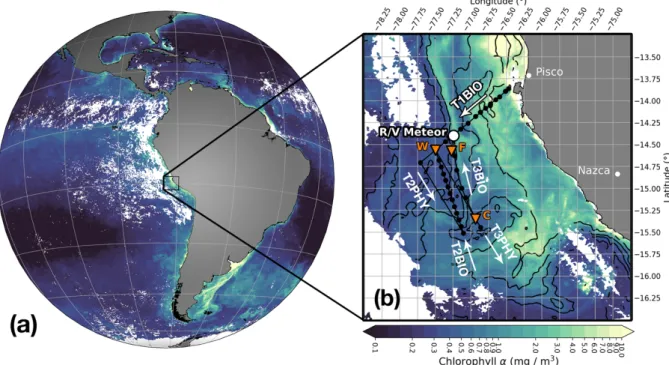
Figure 3: Surface chlorophyllαmeasured from satellite (a) in April 2017 (monthly composite) and (b) on April 14, 2017 at 18:25 UTC with the position of R/V Meteor and names of transects superimposed. Black lines with black circles mark the track of the filament survey with CTD stations and orange triangles indicate CTD stations where primary production was measured. Black contours represent the 20.98^◦C, 22.15^◦C, 23.1^◦C, and 24^◦C isotherms of smoothed (2.5 km gaussian window) satellite sea- surface temperature, white areas indicate missing data due to cloud cover.

3 Filament survey

Observing the biogeochemistry of coastal upwelling regions is challenging due to the inherent intermittency of multi-scale physical processes like eddies, filaments and fronts that interact with the biogeochemical cycles. A survey designed to investigate the biophysical coupling at a cold filament near 14^◦S off the coast of Peru was carried out on April 12- 17, 2017 using an adaptive sampling strategy guided by real-time satellite images. The field work was conducted during R/V Meteor cruise M136 which started on April 11 and ended on April 29, 2017 in Callao, Peru and carried out as part of the "SFB754 - Climate-Biogeochemistry Interactions in the Tropical Ocean" project. The cruise track

(18)

during the survey consisted of five transects (Fig. 3b). The first transect (T1BIO) mapped the upwelling region in cross-shore direction with conductivity, temperature and depth (CTD) measurements including biogeochemical parameters (O₂, NO⁻₃, NO⁻₂, NH⁺₄) determined from water samples. On subsequent along-shore transects, a cold filament present

~ 100 km southeast of transect T1BIO was crossed byR/V Meteor four times in a zigzag pattern: Twice with high-resolution physical underway CTD measurements heading in southeast direction (T2PHY, T3PHY; Fig. 15) and two more times with station-based lowered CTD measurements including biogeochemical parameters heading in northwest direction (T2BIO, T3BIO; Fig. 14; 17). A dense sampling strategy with 8 - 10 km horizontal spacing between stations and 5 - 10 m vertical spacing between samples was applied for the biogeochemical transects. The physical underway transects were completed in under 8 hours and thus closely represent a synoptic view of the surface ocean.

3.1 Hydrographic and meteorological measurements

Hydrographic data was obtained from lowered conductivity, temperature and pressure (CTD) measurements using SeaBird SBE 9-plus CTD system equipped with two sets of pumped sensors. Water samples for oxygen, nutrients and salinity were taken using 24 Niskin bottles (10 l) mounted on a General Oceanics rosette. Salinity samples were analyzed on board with a Guildline Autosal 8 model 8400B salinometer to cali- brate conductivity measurements to practical salinity (PSS-78) with an uncertainty of 0.003 g kg⁻¹. Practical salinity was converted to absolute salinity (TEOS-10) using rou- tines of the Gibbs Seawater toolbox (https://github.com/TEOS-10/GSW-Python). The CTD was also equipped with an oxygen sensor and a WET Labs (USA) fluorometer.

The oxygen sensor was calibrated to an accuracy of 1.5 µmol using Winkler titration.

Because Winkler titration is not reliable in the core of the OMZ and results in too high values (Thomsen et al., 2016b), a concentration of 0µmol l⁻¹was assumed and the profiles corrected accordingly. As the Chlα concentrations determined from water samples were not significantly different from those measured by the fluorometer, the original factory calibration provided by the sensor manufacturer WET Labs (USA) was used. For more

(19)

3.2 Biogeochemical measurements

details on calibration of Chlα fluorescence measurements, the reader is referred to Logi- nova et al. (2016). Underway subsurface temperature and salinity were measured using a Teledyne Oceanscience (Poway, USA) RapidCAST system acquiring profiles of the upper 70 m of the water column every 2 minutes resulting in a horizontal resolution of 500 - 900m depending on the vessel speed. Subsurface current velocities on R/V Meteor were recorded by a vessel-mounted acoustic Doppler current profiler (vmADCP). The system used was a Teledyne RD Instruments OceanSurveyor 75kHz ADCP capable of reaching a maximum depth of ~ 700m. The shallowest velocity measurements were acquired in a bin centered 18 m below the sea-surface. On transects T2PHY and T3PHY the vessel speed was kept nearly constant at ~ 5 m s⁻¹ to obtain high-quality velocity measurements (Fig.

15g,h). Wind speed and direction on R/V Meteor were measured at 35.5 m height with a temporal resolution of one minute.

3.2 Biogeochemical measurements

Nutrient concentrations were determined onboard the ship by a QuAAtro autoanalyzer (SEAL Analytical, Southampton, UK) using standard photometric methods (Grasshoff et al., 1983). Primary production rates were measured by incubation from water samples taken at three CTD stations (orange triangles in Fig. 12) and three depths per station (Fig. 14c; 18c). Samples were taken in quadruplicate into 4.5 l polycarbonate bottles and subsequently in one of three incubators with continuously flowing surface sea water between -4/+10^◦C of the in-situ temperature shaded to 20% , 10% and 1% surface irra- diance (Lee Filters, Seattle, WA, USA) depending only on the sampling depth and not on the in-situ photosynthetically available radiation (PAR). The samples were incubated for a total of 48 hours. After 24 hours of incubation, three bottles were amended with

13C labeled bicarbonate solution (H¹³CO⁻₃) while one bottle was amended with unlabeled bicarbonate solution and air to determine background natural abundance of ¹³C. After another 24 hours of incubation, the samples were filtered, dried and pelletized. Particu- late organic C and the relative abundance of¹³C was then determined through continuous

(20)

flow isotope ratio mass spectrometry coupled to an elemental analyzer. For a more detailed description of the sample processing and the equations used to calculate the carbon fixation rate from the relative abundance of ¹³C , the reader is referred to Krupke et al.

(2015).

3.3 Satellite measurements

To guide the shipboard measurements and put them into a regional context MODIS (Mod- erate Resolution Imaging Spectroradiometer) Level 2 along-track sea-surface temperature (SST) and chlorophylla(Chlα) products with an approximate resolution of 1 km from the TERRA and AQUA satellites were used (https://oceandata.sci.gsfc.nasa.gov/).

We restricted our analysis to daylight images of SST and used the cloud mask based on ocean color because of obvious deficiencies of the cloud mask based on infrared SST data alone. In addition, the April 2017 composite of Chlα images was downloaded from NASA (https://neo.sci.gsfc.nasa.gov). SST data from AVHRR (Advanced Very High Resolution Radiometer) at 25 km resolution was downloaded from NOAA (ftp://

eclipse.ncdc.noaa.gov/pub/OI-daily-v2/NetCDF/). To relate the shipboard current velocity measurements to the synoptic mesoscale circulation during the cruise, geostrophic surface velocities derived from satellite altimetry processed by the SL-TAC multimission altimeter data processing system (SEALEVEL_GLO_PHY_L4_NRT_OBSERVATIONS_008_046) were downloaded from CMEMS (Copernicus Marine Environment Monitoring Service, http://marine.copernicus.eu). Primary production estimates based on the VGPM model (Behrenfeld and Falkowski, 1997) and Chlαmeasurements from the VIIRS satellite at weekly resolution were downloaded from the Oregon State University Ocean Produc- tivity website (http://www.science.oregonstate.edu/ocean.productivity/).

(21)

3.3 Satellite measurements

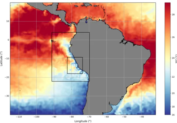
Figure 4: Modeled sea-surface temperature (SST) on April 14, 2017 in the coarse- (1/9^◦) and high-resolution (1/45^◦) simulations superimposed on AVHRR satellite SST. Black rectangles indicate model domains of the coarse- and high-resolution nests.

(22)

4 Coupled Physical-Biogeochemical Model

4.1 Physical model

ROMS (Regional Oceanic Modeling System) is a free-surface, terrain-following coordi- nate model that solves the Primitive Equations using the Boussinesq approximation and a hydrostatic vertical momentum balance. A detailed description including the numerical schemes is given in Shchepetkin and Mcwilliams (2004). The model was configured as a nested set of two spatial domains using an offline, one-way embedding procedure (Fig. 4). The outer domain has a resolution 1/9^◦ over a region of 2207 km in zonal direction by 2911 km in meridional direction (24.4^◦x 26.2^◦), and the inner domain has a resolution of 1/45^◦ over a region of 918 km in zonal direction by 973 km in meridional direction (8.69^◦x 8.76^◦). There are 32 vertical sigma-levels, the resolution varies with water depth and amounts at the surface to 1 - 2 m on the shelf and 5 m offshore. The model topography was derived from the GEBCO (General Bathymetric Chart of the Oceans, http://www.gebco.net) product, interpolated onto the model grid and smoothed to re- duce pressure gradient errors. The lateral open boundary conditions of the outer domain for temperature, salinity, velocities and sea-level were provided at 1/12^◦ resolution by the MERCATOR model (https://www.mercator-ocean.fr) which assimilated in-situ data transmitted fromR/V Meteor during cruise M136, as well as satellite SST and sea-level measurements. The open boundary conditions for oxygen, nitrate, phosphate and silicate were provided at 1/2^◦ resolution by the CARS (CSIRO Atlas of Regional Seas) climatology (Ridgway et al., 2002); for dissolved inorganic carbon (DIC), dissolved organic carbon (DOC) and iron, model output from a global 2^◦x 2^◦ NEMO-PISCES simulation was used (Aumont et al., 2015b). The model was forced with surface wind stress derived from the daily level-2 wind product provided by the ASCAT scatterometer flying on the MetOp-B satellite (https://podaac.jpl.nasa.gov/dataset/ASCATB-L2-25km).

The net surface heat flux Q is given by the COADS (Worley et al., 2005) climatology relaxed toAVHRR(Advanced Very High Resolution Radiometer;ftp://eclipse.ncdc.

noaa.gov/pub/OI-daily-v2/NetCDF/) daily SST according to

(23)

4.2 Biogeochemical models

Q=Q_COADS− dQ

dT ·(SST_ROMS−SST_AVHRR) (1)

where ^dQ_dT represents the additional heat flux that is imposed per degree of temperature difference between model SST and observed SST.

After a spinup of 14 years for the 1/9^◦simulation withPISCES biogeochemistry, the 1/9^◦ simulation withBioEBUS biogeochemistry and both 1/45^◦ simulations were started from this model state and run from January 2013 until April 2017.

4.2 Biogeochemical models

The concentration of a tracer C_i in ROMS is given by

∂C_i

∂t =−∇ ·(uC_i) +K_h∇²C_i+ ∂

∂z(K_z∂C_i

∂z ) +BIO(C_i) (2) with terms on the right-hand side representing (1) advection (2) horizontal diffusion (3) vertical mixing and (4) a residual caused by biogeochemical processes.

The biogeochemical models that ROMS was coupled to in our different simulations were PISCES and BioEBUS, both of which will be described in the following. The config- uration of the physical model was identical with two exceptions: (1) The lateral tracer mixing acted on isopycnal surfaces (TS_MIX_ISO) in the PISCES simulations and on geopotential surfaces (TS_MIX_GEO) in the BioEBUS simulations. (2) A newer version of the surface boundary layer mixing parameterization (LMD_SKPP2005) was used in the BioEBUS simulations than in the PISCES simulations. While no rigorous testing on the effects of these differences has been done, the seasonal cycle of the average mixed-layer depth was similar in all simulations and we assume effects to be small. The mesoscale variability (i.e. the position of mesoscale eddies) was different in the PISCES and BioEBUS simulations, which may also be related to the choice of parameterizations. However, in the turbulent mesoscale regime large differences resulting from small perturbations such as those generated by numerical errors are generally expected. The differences between simulations that were run on separate machines can thus likely be attributed to these

(24)

numerical differences.

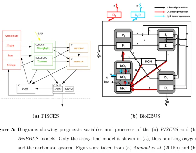
ThePISCES (Pelagic Interaction Scheme for Carbon and Ecosystem Studies) model simu- lates the biogeochemical cycles of carbon and the main nutrients (P, N, Si, Fe). It includes two phytoplankton compartments (nanophytoplankton and diatoms), two zooplankton size classes (microzooplankton and mesozooplankton), two detritus classes termed small particulate organic carbon (1 - 100µm, POC) and big particulate organic carbon (100 - 5000 µm, GOC) and a description of the carbonate chemistry. The sinking velocities for the detritus classes are constant for POC (3 m d⁻¹) and increasing from a minimum value (50 m d⁻¹) at the surface to a maximum value (200 m d⁻¹) at 5000 meters depth for GOC. In our configuration,PISCES is not coupled to a sediment model which could act as a reservoir for POC and DOC. Particles that reach the bottom are immediately converted to dissolved organic carbon (DOC) and subsequently remineralized. A detailed model description is given in Aumont et al.(2015b).

The BioEBUS (Biogeochemical model for the Eastern Boundary Upwelling Systems) model is nitrogen-based and includes nitrate, nitrite and ammonium as prognostic variables. The complex nitrogen cycle allows nitrification, denitrification and annamox, which are important processes in oxygen minimum zones (Kalvelage et al., 2013) to be explicitly represented. However, the model lacks the nutrients phosphate, silicate and iron which are present inPISCES. Similar to PISCES, BioEBUS includes two phytoplankton compartments (nanophytoplankton and diatoms), two zooplankton size classes (microzooplankton and mesozooplankton) and two types of detritus (POC and GOC). The sinking velocities for the detritus classes are constant at 1 m d⁻¹ (POC) and 40 m d⁻¹ (GOC) respectively.

BioEBUS includes a sediment model and a cumulative layer exists at the sediment-water interface where sinking particles are stored without further interaction with the water column. A detailed model description is given inGutknecht et al. (2013).

Both biogeochemical models have in common that they use two compartments each for

(25)

4.3 Impact of increased horizontal resolution

(a) PISCES (b) BioEBUS

Figure 5: Diagrams showing prognostic variables and processes of the (a) PISCES and (b) BioEBUS models. Only the ecosystem model is shown in (a), thus omitting oxygen and the carbonate system. Figures are taken from (a)Aumont et al.(2015b) and (b) Gutknecht et al.(2013), respectively.

the representation of phytoplankton, zooplankton and detritus. The main advantages of each model are a more complex nitrogen cycle and a sediment model inBioEBUS and the explicit representation of phosphate, silicate, iron and carbonate chemistry in PISCES.

4.3 Impact of increased horizontal resolution

Two simulations at coarse (1/9^◦) and high (1/45^◦) horizontal resolution with the same 32 vertical levels were run with each of the two biogeochemical models. To assess the effect of increased horizontal resolution, we interpolated the high-resolution simulations on the coarse-resolution grid and analyzed the difference. Mesoscale eddies dominate the differences between the BioEBUS and PISCES simulations on timescales of several months. We identified 2 years as a useful averaging period to compare simulations that exhibit substantial differences on the mesoscale. Because the BioEBUS simulations were

(26)

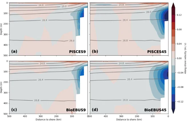
Figure 6: Along-shore currents in the (a) PISCES9 (c) BioEBUS9 (b) PISCES45 and (d) BioE- BUS45 simulations, averaged on depth levels in along-shore direction with 25 km cross-shore bins in a coastal band of 500 km width between 10.5^◦S and 17.5^◦S over the period 2015 - 2016.

only started in 2013 from the PISCES9 initial conditions, the first two years were not used and all following analysis is based on averages over the period 2015 - 2016, assuming a sufficient adjustment of the relatively fast near-surface biogeochemistry by this time.

The mean kinetic energy (MKE) increased between the coarse- and high-resolution simulations especially near the coast (not shown), which manifests most notably as an increase in the mean along-shore currents (Fig. 6). The poleward undercurrent that is seen near the shelf break at ~ 100 m depth extends ~ 20 km further offshore and is ~ 4 cm s⁻¹stronger in its core in the 1/45^◦ compared with the 1/9^◦ simulations. This result is consistently found in both sets of simulations (PISCES & BioEBUS) and the stronger undercurrent is closer to observed values of 10 - 15 cm s⁻¹ (Chaigneau et al., 2013). No substantial

(27)

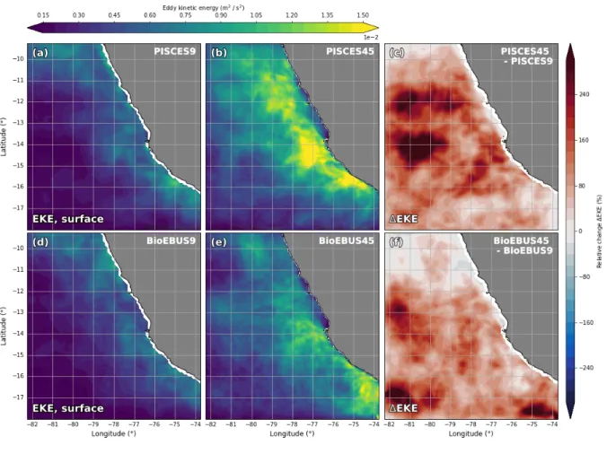
changes in the cross-shore circulation are discernible (not shown). Two factors are likely responsible for the changes in strength and shape of the poleward undercurrent in our simulations: Firstly, the smoothing of the model topography can be reduced at higher resolution, leading to a steeper shelf break. Secondly, numerical diffusion is reduced at higher resolution i.e. previously subgrid-scale precesses are explicitly resolved a contribute to the average kinetic energy. In addition to the mean circulation, the eddy kinetic energy (EKE) increased in the 1/45^◦ compared with the 1/9^◦ simulations as apparent in surface EKE fields (Fig. 7). The change in EKE between the coarse- and high-resolution simulations is positive almost everywhere, small areas of negative EKE change are only found in the BioEBUS45 simulation north of 12^◦S and in the PISCES45 simulation in the southeast corner of the model domain. The strongest absolute change is seen in a coastal band 100 km in width with a maximum near Pisco (2·10⁻³ m²s⁻²). The EKE increase in the BioEBUS simulations (1·10⁻³ m²s⁻²) is smaller than in the PISCES simulations (2·10⁻³ m²s⁻²) and the highest EKE values occur in different locations, at 14.5^◦S in PISCES and near the coast at 17^◦S in BioEBUS. In contrast, the largestrelative changes are found between 100 - 200 km offshore where low EKE (< 2·10⁻⁴ m²s⁻²) is found in the coarse-resolution simulations and range from -75 % to 500 % locally. Averaged over the model domain an increase in surface EKE by 89% and 113% is observed in the PISCES and BioEBUS simulations, respectively. A band of ~ 200% EKE increase around 12^◦S in the PISCES simulations (Fig. 7c) coincides with a persistent filament that formed there repeatedly (not shown). The increases in MKE (not shown) and EKE (Fig. 7) around 12^◦S could be related to a topographic bend in the coastline that favors the generation of filaments in this area in the high-resolution simulations but is not present due to smoothed topography in the coarse-resolution simulations. EKE of > 1.2·10⁻³m²s⁻² is not found north of 13^◦S in the BioEBUS45 simulation, which is where the strongest EKE increase occurred in the PISCES45 simulation, the reason of which remains unclear. In general, the PISCES and BioEBUS simulations agree qualitatively on the result of increased EKE in the high-resolution simulations, but magnitude and locations of these changes exhibit considerable differences. Although only the changes in surface EKE are described here,

(28)

similar changes in EKE were found at the subsurface (not shown).

Consistent vertical patterns of relative changes in the biogeochemical fields emerge when we subtract average cross-shore sections of the coarse-resolution simulations from the corresponding sections in the high-resolution simulations (Fig. 8). Note that in contrast to Figure 7, only the changes in the mean fields and not the mean fields themselves are shown.

The effect on the distribution of oxygen and nitrate is greatest around theσ_θ= 25.6 kg m⁻³ isopycnal that approximately coincides with the 10µmol l⁻¹ NO⁻₃ nutricline (not shown), where an O₂ increase by ~ 20µmol l⁻¹ and a nitrate decrease by 2.5µmol l⁻¹ is observed.

An area of negative change in oxygen (−15 µmol l⁻¹) with a vertical extent of ~ 100 m is found slightly deeper around the 26 kg m⁻³ isopycnal at 350 - 500 km offshore. An O₂ increase (+5 µmol l⁻¹) and NO⁻₃ decrease (−0.75 µmol l⁻¹) is found 100 m below the pycnocline within 300 km from the coast. Between 200 - 300 m changes in O₂ are positive but small (< 2.5µmol l⁻¹) while changes in NO⁻₃ are negative (−0.75µmol l⁻¹) in BioEBUS but inconclusive in PISCES. At first glance, considerable differences in the NO⁻₃ changes from coarse to high resolution seem to exist between the PISCES and BioEBUS simulations: While both postitive and negative NO⁻₃ changes are visible in PISCES, negative changes dominate in the BioEBUS simulations (Fig. 8e,f). On closer inspection the patterns of NO⁻₃ change appear very similar in PISCES and BioEBUS but exhibit an offset of ~ 1.5µmol l⁻¹, which could be related to differences in the mean NO⁻₃ fields between the two biogeochemical models (Fig. 10e,f). The pattern correlation between the opposing O₂ and NO⁻₃ changes around the nutricline is therefore high. An increase in Chlα concentration (+ 0.3 mg m⁻³) centered around the nutricline coincides with the changes in O₂ and NO⁻₃ described above. A surface Chlα decrease of ~ 0.6 mg m⁻³ in PISCES and ~ 0.3 mg m⁻³ in BioEBUS is apparent, which coincides with a NO⁻₃ increase (+1µmol l⁻¹) in PISCES but a NO⁻₃ decrease(−0.5µmol l⁻¹) in BioEBUS. Chlαchanges below ~ 100 m are negligible (< 0.05 mg m⁻³) due to low mean Chlα concentrations at these depths (not shown).

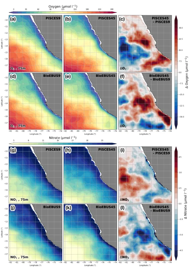
In order to identify horizontal patterns associated with the O₂and NO⁻₃ changes described above (Fig. 8a,b,e,f) their average distributions at 75 m depth are investigated (Fig. 9a-l).

(29)

Figure 7: Surface eddy kinetic energy for the (a) PISCES9 (d) BioEBUS9 (b) PISCES45 and (e) BioEBUS45 simulations, averaged over the period 2015-2016. Panels (c,f) show the relative change in EKE with increased resolution calculated as ∆EKE = EKE1/45^◦ - EKE1/9^◦ for the (c) PISCES and (f) BioEBUS simulations. The velocity fields were interpolated at the given depths using ROMSTOOLS (Penven et al., 2007) functions translated from the original Matlab code into the Python programming language (https://github.com/jaard/romstools-visual). Eddy velocities were calculated using a Reynolds decomposition with u⁰ = u− hui_30d and v⁰ = v− hvi_30d, where u and v are the daily (PISCES) / 3-day (BioEBUS) average zonal and meridional velocity components, respectively and hi_30d denotes a 30-day moving average. The eddy kinetic energy per unit mass is then given by EKE = ¹₂ ·(u⁰²+v⁰²).

(30)

Figure 8: Relative changes in (a,b) Oxygen (c,d) Chlorophyll a and (e,f) Nitrate between the 1/9^◦ and 1/45^◦ simulations calculated as (a,c,e) ∆PISCES = PISCES45 - PISCES9 and (b,d,f) ∆BioEBUS = BioEBUS45 - BioEBUS9, respectively. All fields were averaged on depth levels in along-shore direction with 25 km cross-shore bins in a coastal band of 500 km width between 10.5^◦S and 17.5^◦S over the period 2015 - 2016. Grey lines represent potential density averaged over BioEBUS9 / BioEBUS45 and PISCES9 / PISCES45, respectively.

(31)

4.4 Impact of biogeochemical model choice

An oxygen increase (+35 µmol l⁻¹) is apparent at 14^◦S about 50 km offshore and at 16^◦S within 20 km from the coast (Fig. 9c,f) in both PISCES and BioEBUS simulations. In precisely the same locations a nitrate decrease in PISCES (−3 µmol l⁻¹) and BioEBUS (−5 µmol l⁻¹) is found (Fig. 9i,l). A decrease in oxygen (−35µmol l⁻¹) occurs ~ 200 km offshore at 14^◦S in PISCES and ~ 100 km offshore near 17^◦S in BioEBUS. Again, nitrate changes of opposing sign (+5 µmol l⁻¹ PISCES / +4 µmol l⁻¹ BioEBUS) are present in the same locations. Thus, the changes in NO⁻₃ and O₂ at 75 m depth show a very high spatial correlation similar to the vertical sections and and exhibit a ratio of approximately 8 : 1.

Summarizing, an increased horizontal resolution from 1/9^◦ to 1/45^◦ leads to an average increase in eddy kinetic energy by about a factor of 2 in our simulations. While the PISCES and BioEBUS simulations agree qualitatively on this result, they differ in the magnitude of the increase. Mean kinetic energy likewise increases, manifesting as an increase in velocity of the poleward undercurrent by 30% which is closer to observations.

An increase in the cross-sectional area of the undercurrent seems to be related to changes in the model topography. The effect of horizontal resolution on the biogeochemical fields is greatest around the nutricline within 250 km from the coast, where an oxygen increase by +20 µmol l⁻¹, a nitrate decrease by −2.5 µmol l⁻¹ and a Chlα increase by +0.3 mg m⁻³ are present. High vertical and horizontal pattern correlation of the opposing changes in O₂ and NO⁻₃ is seen in the simulations with the ∆O₂: ∆NO⁻₃ ratio between these changes being approximately 8 : 1. While an offset exists between PISCES and BioEBUS especially for NO⁻₃, the characteristic patterns of the changes in average vertical sections and horizontal fields are remarkably similar for the PISCES and BioEBUS, suggesting independence of the biogeochemical model used and thus encouraging some confidence in the robustness of the results.

4.4 Impact of biogeochemical model choice

The same method as above is applied to quantify the differences between the PISCES and BioEBUS biogeochemical models at both 1/9^◦and 1/45^◦ horizontal resolution. Similarly,

(32)

Figure 9: (a,b,d,e) Oxygen and (g,h,j,k) nitrate at 75 m depth averaged over the period 2015 - 2016 and their relative changes between the 1/9^◦ and 1/45^◦ simulations calculated as (c,i) ∆PISCES = PISCES45 - PISCES9 and (f,k) ∆BioEBUS = BioEBUS45 - BioEBUS9, respectively.

(33)

consistent vertical patterns of relative changes in the biogeochemical fields emerge when average cross-shore sections of the PISCES simulations are subtracted from the corresponding sections in the BioEBUS simulations, which can be understood as the effect of choosing BioEBUS over PISCES.

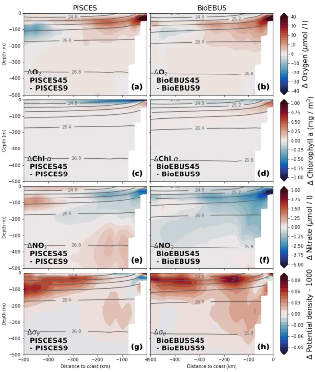
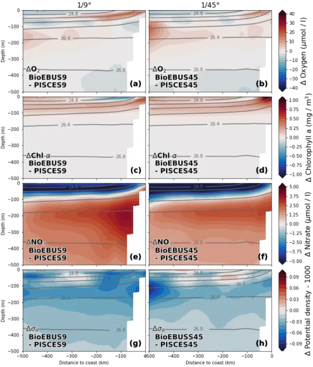
The choice of a particular biogeochemical model can have a similarly strong impact on the average cross-shore distributions of oxygen, chlorophyll α and nitrate as horizontal resolution (Fig. 10). A positive difference in oxygen (+20 µmol l⁻¹) Between BioEBUS and PISCES, centered around the σ_θ = 25.6 kg m⁻³ isopycnal is present within 100 km and 250 km from the coast in the coarse- and high-resolution simulations, respectively (Fig. 10a,b). O₂ concentrations in the oxygen minimum zone below 300 m depth are 2 - 5 µmol l⁻¹ lower in BioEBUS than in PISCES, with largest difference of 5 µmol l⁻¹ occurring at 500 m depth near the shelf. On average, positive and negative differences in O₂ approximately compensate each other. The difference in Chlα between the two biogeochemical models exhibits a horizontal dipole pattern with high (+0.75 mg m⁻³) values within 50 km from the coast, indicating a difference in the cross-shore gradient and suggesting that primary production occurs closer to the shore in BioEBUS than in PISCES (Fig. 10c,d). On average, Chlαconcentrations in the upper 100 m are higher (+

0.3 mg m⁻³) in BioEBUS than in PISCES. A substantial difference in the vertical NO⁻₃ gradient (±5 µmol l⁻¹/100 m) between the two biogeochemical models is apparent, with NO⁻₃ concentrations in the BioEBUS simulations being lower (−5 µmol l⁻¹) in the upper 100 m and higher (+5 µmol l⁻¹) at 200 m depth compared with the PISCES simulations, resulting in a distinct dipole pattern across the nutricline (Fig. 10e,f). The area of lower NO⁻₃ and higher Chlαin BioEBUS than in PISCES coincide. Subsurface potential density is on average lower (−0.02 kg m⁻³) in BioEBUS than in PISCES, pointing to unintended physical differences between the simulations, e.g. (numerical) diffusion or surface heat flux (Fig. 10g,h). Differences in potential density on scales of O(10) km between PISCES and BioEBUS which could be related to mesoscale differences between the simulations exhibit patterns that are correlated with differences in oxygen concentration (Fig. 10a,b,g,h).

(34)

In summary, the differences in the simulated biogeochemical fields due the use of either the PISCES or BioEBUS model are of similar magnitude as the impact of increased horizontal resolution. Oxygen locally exhibits positive and negative differences between PISCES and BioEBUS simulations which cancel out on average. A stronger cross-shore surface Chlαgradient and higher Chlαconcentrations above the nutricline are present in BioEBUS compared with PISCES. Nitrate shows the most pronounced differences between the PISCES and BioEBUS simulations, which reveal a substantial bias in the vertical NO⁻₃ gradient. Lower NO⁻₃ concentrations above the nutricline in BioEBUS coincide with the area of higher Chlα concentrations.

(35)

Figure 10: Relative change in (a,b) Oxygen (c,d) Chlorophyll a and (e,f) Nitrate between the BioEBUS and PISCES simulations so that positive changes represent higher values of the respective variables in the BioEBUS simulations (BioEBUS minus PISCES).

Averaging procedure similar as in Figure 6. Grey lines represent potential density averaged over BioEBUS9 / PISCES9 and PISCES45 / BioEBUS45, respectively.

(36)

5 Characterization of an observed cold filament

5.1 Oceanographic setting

The upwelling region along the coast is characterized by relatively steady equatorward winds that are largely parallel to the shore and sustain upwelling over the entire year (Strub et al., 1998). The coldest and most persistent upwelling center along the coast is located near 15^◦S off Pisco (Zuta and Urquizo, 1972) and characterized by distinct maxima in mean and variance of the wind speed (Stuart, 1981; Rahn and Garreaud, 2013; Astudillo et al., 2017) and wind stress curl (Bakun and Nelson, 1991). Sea-surface temperature near the coast is inversely correlated with the strength of these predominant along-shore winds and follows their seasonal cycle (Stuart, 1981; Dewitte et al., 2011), consistent with the mechanism of wind-induced upwelling through Ekman transport and Ekman pumping (Sverdrup et al., 1942). The wind-driven gyre circulation maintains a generally northward surface flow within the Humboldt current, but the near-surface limb of the poleward undercurrent centered at 150 m depth near the shelf may outcrop

~ 100 km from the coast (Penven et al., 2005). The strongest upwelling-favorable winds near Pisco occur in Austral fall and winter (Dewitte et al., 2011;Rahn and Garreaud, 2013) and are out of phase with the most intense phytoplankton blooms that occur in Austral summer, when a shallow mixed-layer concentrates phytoplankton near the well-lit surface and thus prevents dilution and light limitation (Echevin et al., 2008). With respect to this seasonal cycle, the filament survey that was carried out on April 12 - 17, 2017 at the end of Austral summer falls in a period of moderate but increasing wind speed and mixed-layer depth. Moderate winds (5 - 6 m s⁻¹) from south-southeast were observed close to the coast (~ 30 km) during transit ofR/V Meteor from Callao to the study area near Pisco on April 11-12 (Fig. 11). The wind speed increased to 8 m s⁻¹ at ~ 50 km distance to the first CTD station near the Paracas peninsula. Once the vessel escaped the immediate influence of the coast and started moving offshore on transect T1, the wind turned slightly onshore to southerly directions and highly variable winds with maxima of > 12 m s⁻¹ were observed within ~ 50 km from the coast. The fluctuations in wind speed and direction in this near-

(37)

5.1 Oceanographic setting

shore area seem to approximately correspond to a diurnal cycle and suggest the influence of the land-sea wind, which has been shown to be an important type of variability in the area (Burt et al., 1973). Offshore of the coastal wind speed maximum the winds diminished again to ~ 8 m s⁻¹ from southeasterly directions. The highest wind speeds of the survey (11 - 14 m s⁻¹) from southeasterly directions were observed on April 14 - 15 at 100 - 160 km distance from the coast on cross-shore transect T1 and the northern half of along-shore transect T2PHY. It is quite striking that the areas of high wind speed and high sea-surface temperature (> 24^◦C) approximately coincide and that the transition from moderate (9 m s⁻¹) to high (14 m s⁻¹) winds occurs almost exactly at the upwelling front, which points to the possible relevance of SST-wind coupling (Oerder et al., 2016).

A layer of clouds that is confined to the warm offshore waters downwind of transect T1 (Fig. 11, pink contour) supports this hypothesis. Between April 15 - 17 on a zigzag course that is formed by transects T2BIO, T3PHY and T3BIO southeasterly winds of 7 - 9 m s⁻¹ were present, only briefly increasing to > 11 m s⁻¹ on April 16 over the warm water close to transect T1. Throughout the survey, winds were directed approximately parallel to the coastline. Changes in the mean wind speed during the survey are difficult to estimate due to the high spatial variability. However, two later crossings of transect T1 suggest that the mean wind decreased by ~ 2 m s⁻¹ between April 14 and April 16 - 17.

The cold upwelling center near 15^◦S is readily discernible in satellite images of sea surface temperature (SST) and chlorophyll α(Chlα) taken on April 14th at 18:25 UTC (Fig.

12b). The dominant feature is a strong cross-shore temperature gradient between warm (24.5^◦C) offshore waters and the cold (17^◦C) upwelling region along the coast between Pisco and Nazca. Protruding offshore from the upwelling region are two cold filaments with temperatures of 21.5^◦C and ~ 20.5^◦C in their respective centers, separated by a

~ 30km wide intrusion of 1^◦C warmer water between them. The along-shore temperature difference compared to the waters surrounding both filaments is 2.5^◦C. The location of the filaments in along-shore direction resembles the location of the two upwelling patches near Pisco and Nazca, suggesting that they carry recently upwelled water originating in these patches. The northern filament is extending southwestward from 15^◦S, 77.75^◦W

(38)

Figure 11:Direction and velocity of 1-minute wind measured at 35.5 m height between April 9 - 17, 2017. Color and length of arrow indicate wind speed, data is subsampled so that spacing between arrows is ~ 8 km. The black line indicates the cruise track, black circles mark the position of R/V Meteor at 00:00 UTC on the given dates.

The grayscale image represents satellite sea-surface temperature (SST) on April 14 (see Fig. 12a), with black and white colors corresponding to < 16^◦C and > 24.25^◦C, respectively. The light pink contour indicates missing data due to cloud cover.

(39)

to 15.5^◦S, 77.3^◦W, its width being ~ 20km on average and less than 10km at its narrow- est point near 15.5^◦S, 77^◦W. The southern filament is more than twice as wide, so that the along-shore extent of the two filaments combined is > 100km. Here we focus on the smaller northern filament, because numerous in-situ measurements exist there. The cross- shore gradient in SST is reflected by a similar gradient of Chlα concentration between the coastal upwelling (5 mg m⁻³) and the offshore waters (< 0.2 mg m⁻³), suggesting an inverse correlation of SST and Chlα (Fig. 12b). This correlation does not exist in the bay of Pisco (13.5^◦S, 76.3^◦W), where very high Chlαconcentrations of > 10 mg m⁻³ but similarly high SST (> 24^◦C) are present. The maximum Chlα values associated with the northern and southern filaments are ~ 1 mg m⁻³ and ~ 3 mg m⁻³, respectively. Another Chlα maximum (~ 3 mg m⁻³) is found along the main upwelling front ~ 100 km offshore, marked by a high SST gradient and a temperature of ~ 22.5^◦C. The Chlα maximum of the northern filament is located at its northern edge as opposed to its core. It is in- distinguishable from the Chlα maximum associated with the upwelling front offshore of transect T2PHY. The relative location of the associated Chlα maximum to the southern filament is unclear.

So far, the surface structure of the coastal upwelling and the associated filaments was discussed. In the following we will first describe the cross-shore structure of the upwelling region and then move on to a characterization of the observed filament in terms of both physical and biogeochemical variables based on 5 vertical transects.

The vertical cross-shore structure of the upwelling region from the coast to ~ 160 km offshore is seen Figure 14. Both maximum (25^◦C) and minimum (12^◦C) temperatures on the transect occur offshore, at the surface and at 100m depth, respectively (Fig. 14b).

Maximum (35.5 g kg⁻¹) and minimum (34.75 g kg⁻¹) salinity are found at the same respective locations (Fig. 14d). These extreme values are separated by a sharp transition between 20 m - 50 m depth. The vertical gradient weakens towards the shelf as both variables show opposite cross-shore gradients at the surface and at depth. Below ~ 80 m depth

(40)

Figure 12:Satellite images of (a) SST and (b) Chlorophyll α from MODIS, taken at 18:25 UTC on April 14, 2017 (c) the absolute gradient of smoothed SST (3 km window) and (d) the geostrophic velocity on April 14, 2017 based on satellite altimetry with streamlines of the flow superimposed. The position of R/V Meteor at this time is marked by the white filled circle. Note the power law and logarithmic scaling for SST and Chlα, respectively. Black contours in (a,b,d) represent the 20.98^◦C, 22.15^◦C, 23.1^◦C, and 24^◦C isotherms of a smoothed SST field (2.5 km gaussian window). Black lines with filled circles indicate the cruise track and locations of CTD stations, orange triangles in (b) mark three CTD stations (W - warm, F - front, C - cold filament) where primary production was measured in addition to the regular parameters (Fig. 16). White areas in (a,b,c) were covered by clouds during overpass of the MODIS satellite and are therefore masked, grey areas are land.

(41)

both temperature and salinity are higher near the shelf (14^◦C, 35 g kg⁻¹) than in the open ocean (13^◦C, 34.75 g kg⁻¹). The lowest sea-surface temperature (SST) of 17^◦C occurs on the shelf in the upwelling patch near Pisco (Fig. 14b). SST in the survey area almost continuously increases offshore, accompanied by an increase in mixed-layer depth from 5 m to 30 m and a decrease in density from 1025.5 kg m⁻³ to 1024 kg m⁻³. An exception from this average cross-shore gradient is a 10 km wide cold anomaly of 1^◦C at 40 km cross-shore distance, coinciding with both an upward displacement of the 1025 kg m⁻³ isopycnal and a deepening of the mixed-layer by 10m, respectively (Figs. 14b). The cold anomaly can be related to a small filament discernible in Figure 12a extending northward across transect T1 from the upwelling patch. The filament is associated with a small northward velocity anomaly in a predominantly southward current, resulting in high horizontal velocity shear (0.6 m s⁻¹/ 20 km) on its offshore side (Fig. 14h). The prevailing southward flow of 0.2 - 0.3 m s⁻¹ within 120 km from the coast is in good agreement with geostrophic current estimates from satellite altimetry (Fig. 12d). The strongest cross-shore SST gradient (0.2 ^◦C km⁻¹) occurs 20 km from the coast. A slightly smaller peak (0.15^◦C km⁻¹) is found 110 km offshore, approximately at the outcrop of the 1024 kg m⁻³ isopycnal.

This is the location of the main along-shore upwelling front separating cold coastal and warm offshore waters (Fig. 12a). Low SST gradients (< 0.05 ^◦C km⁻¹) are present within 20 km on both sides of the front (Fig. 14b). The presence of several distinct peaks in stratification between 10 - 30 m depth could indicate that the vertical temperature drop by 0.2^◦C in the top 10 m is due to day-time restratification and that the night-time mixed-layer is deeper. The lowest sea-surface salinity (SSS) of 35 g kg⁻¹ occurs at 20 km offshore, just eastward of the cold anomaly described above (Fig. 14d). SSS between 40 km and 100 km offshore is almost uniform at ~ 35.25 g kg⁻¹ in the upper 30 m, one exception being a slight fresh anomaly of 0.05 g kg⁻¹ along the 21^◦C isotherm. Another narrow (~ 1 km) fresh anomaly of the same magnitude appears just east of the main SST front 100 km along the transect. Below the mixed-layer (45 m) in the middle of the transect (70 km) there is a 30 m thick layer of relatively homogeneous temperatures between 17^◦C and 19^◦C, coinciding with a downward displacement of the 1025.5 kg m⁻³