Methane and sulfate dynamics in sediments from mangrove-dominated tropical coastal lagoons, Yucatán, Mexico

(1)

www.biogeosciences.net/13/2981/2016/

doi:10.5194/bg-13-2981-2016

Methane and sulfate dynamics in sediments from mangrove-dominated tropical coastal lagoons, Yucatán, Mexico

Pei-Chuan Chuang¹, Megan B. Young², Andrew W. Dale³, Laurence G. Miller², Jorge A. Herrera-Silveira⁴, and Adina Paytan^1,5

1Department of Earth and Planetary Sciences, University of California Santa Cruz, 1156 High St., Santa Cruz, CA 95064, USA

2US Geological Survey, 345 Middlefield Rd, MS 434, Menlo Park, CA 94025, USA

3GEOMAR Helmholtz Centre for Ocean Research Kiel, Wischhofstr. 1–3, 24148 Kiel, Germany

4CINVESTAV-IPN, Unidad Mérida, A.P. 73 CORDEMEX, Mérida, Yucatán, Mexico

5Institute of Marine Sciences, University of California Santa Cruz, 1156 High St., Santa Cruz, CA 95064, USA Correspondence to:Pei-Chuan Chuang (pchuan2@ucsc.edu)

Received: 14 October 2015 – Published in Biogeosciences Discuss.: 10 November 2015 Revised: 26 April 2016 – Accepted: 27 April 2016 – Published: 23 May 2016

Abstract. Porewater profiles in sediment cores from mangrove-dominated coastal lagoons (Celestún and Chelem) on the Yucatán Peninsula, Mexico, reveal the widespread co- existence of dissolved methane and sulfate. This observation is interesting since dissolved methane in porewaters is typically oxidized anaerobically by sulfate. To explain the observations we used a numerical transport-reaction model that was constrained by the field observations. The model suggests that methane in the upper sediments is produced in the sulfate reduction zone at rates ranging between 0.012 and 31 mmol m⁻²d⁻¹, concurrent with sulfate reduction rates between 1.1 and 24 mmol SO²⁻₄ m⁻²d⁻¹. These processes are supported by high organic matter content in the sediment and the use of non-competitive substrates by methanogenic microorganisms. Indeed sediment slurry incubation experiments show that non-competitive substrates such as trimethylamine (TMA) and methanol can be utilized for microbial methanogenesis at the study sites. The model also indicates that a significant fraction of methane is transported to the sulfate reduction zone from deeper zones within the sedimen- tary column by rising bubbles and gas dissolution. The shallow depths of methane production and the fast rising methane gas bubbles reduce the likelihood for oxidation, thereby allowing a large fraction of the methane formed in the sediments to escape to the overlying water column.

1 Introduction

Wetlands are the largest natural source of methane (CH₄) to the atmosphere, accounting for between 20 and 25 % of the global atmospheric methane budget (Fung et al., 1991;

Whalen, 2005). Methane produced in wetlands is primarily biogenic, originating from microbial activity in anaerobic sediments and soil. Since sulfate-reducing bacteria outcompete methanogens for common substrates (Oremland and Polcin, 1982), freshwater wetlands typically have much higher methane fluxes to the atmosphere than brackish to fully marine wetlands (Bartlett et al., 1985, 1987; Segarra et al., 2013). Marine and estuarine sediments are generally characterized by comparatively low rates of methanogenesis with a methane production and accumulation zone located deeper within the sediment below the sulfate reduction zone (Holmer and Kristensen, 1994; Martens and Klump, 1984;

Poulton et al., 2005; Segarra et al., 2013). In these marine or estuarine systems methane that diffuses upwards towards the sediment surface can be oxidized both anaerobically (AOM) and aerobically within the sediments and in the water column, reducing emissions to the atmosphere (Whalen, 2005).

Despite brackish to marine salinities, methane fluxes com- parable to those measured in freshwater wetlands have been reported for coastal mangrove-dominated lagoon systems in several places around the world, including Florida (Barber

(2)

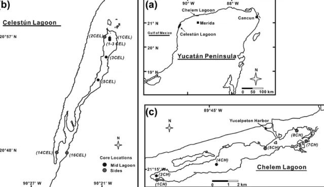
Figure 1.Maps of(a)the Yucatán Peninsula with lagoon locations,(b)Celestún Lagoon and(c)Chelem Lagoon showing the sampling stations (circles) of sediment cores.

et al., 1988), Puerto Rico (Sotomayor et al., 1994), India (Biswas et al., 2004, 2007; Purvaja and Ramesh, 2000, 2001;

Ramesh et al., 1997, 2007; Verma et al., 1999), Tanzania (Kristensen et al., 2008), Thailand (Lekphet et al., 2005), China (Alongi et al., 2005), the Andaman Islands (Linto et al., 2014) and Australia (Call et al., 2015). The anaerobic and organic-rich sediments found in these systems provide a suitable environment for methanogenesis, yet the extensive supply of sulfate from seawater should favor sulfate reducers over methanogens in the shallow sections of the sediments (Kristensen et al., 2008; Lee et al., 2008). There are, however, several possible ways for coastal mangrove lagoons to sustain relatively high methane fluxes despite high sulfate concentrations. For example, if the microbial activity of sulfate reducers is high and sulfate replenishment from the overlying water is slow, sulfate may become depleted in the upper centimeters of the sediment, thus allowing methanogenesis to occur close to the sediment surface. Additionally, methanogens can co-exist with sulfate reducers when non- competitive substrates (those used only by methanogens and not by sulfate reducers) are available. Moreover, in some systems methane may migrate from deeper in the sediment to shallower depth and to the water column. Typically, a large percentage of the methane produced in sediments is oxidized prior to reaching the atmosphere, and in shallow-water systems, the oxidation takes place primarily in the sediments and not in the water column (Martens and Klump, 1980;

Mitsch and Gosselink, 2000; Weston et al., 2011; Segarra et al., 2013, 2015). However, accumulation and transport of

methane in gas bubbles reduces the exposure time of methane to oxidants such as oxygen and sulfate, allowing a large fraction of gas to escape the sediment (Barnes et al., 2006;

Martens and Klump, 1980).

The objective of this study was to examine porewater methane distributions within the sediments of two mangrove- dominated coastal lagoons in Mexico and relate them to sulfate concentrations in sediment porewaters. We aim to gain a better understanding of the factors controlling the methane flux from coastal mangrove-dominated lagoon sediments. To this end, we applied a numerical transport-reaction model based on Wallmann et al. (2006) and Chuang et al. (2013) to simulate porewater methane and sulfate concentration profiles. We also performed sediment slurry incubation experiments to test the effect of competitive and non-competitive substrates on methanogenesis in the lagoon sediments. The results provide quantitative data on methane dynamics in coastal mangrove-dominated lagoon systems and highlight their importance as methane sources to the atmosphere.

2 Study sites

Fieldwork was conducted in two mangrove-dominated coastal lagoons located on the western Yucatán Peninsula, Mexico (Fig. 1). The typical climatological pattern for this area consists of a dry season (March–May), a rainy season (June–October) during which the majority of the an- nual rainfall (> 500 mm) occurs, and the “nortes” season (November–February), which is characterized by moder-

(3)

ate rainfall (20–60 mm) and intermittent high wind speeds greater than 80 km h⁻¹(Herrera-Silveira, 1994).

Celestún Lagoon (20^◦52⁰N, 90^◦22⁰W) is long, narrow, and relatively shallow (average depth=1.2 m). The inner and middle sections of the lagoon always have lower salinities than the section near the mouth due to year-round discharge of brackish groundwater from multiple submarine springs (Young et al., 2008). Salinity within the lagoon fluctuates seasonally, with salinity in the inner zone ranging from 8.9 to 18.2 during the course of this study, grading out to marine salinities at the mouth of the lagoon (Young et al., 2008). The lagoon is surrounded by 22.3 km²of a well-developed mangrove forest, and has experienced relatively little disturbance from human development and/or pollution such as wastew- ater discharge (Herrera-Silveira et al., 1998). Sediments in Celestún consist primarily of autochthonous carbonate ooze.

Chelem Lagoon (21^◦15⁰N, 89^◦45 W; average depth=0.7 m), in contrast, receives very little groundwater input and the surrounding area has been heavily impacted by urban development. Salinity in Chelem ranged from brackish to hypersaline (24.8–40.3 during the study period), and vegetation surrounding the lagoon consists of scrub mangrove forest (Herrera-Silveira et al., 1998). The construction of Yucalpeten Harbor in 1969 (Valdes and Real, 1998) increased the circulation and resulted in sandy marine sediments entering the lagoon. Sediments in Chelem deposited since 1969 consist of a heavily bioturbated mix of sands and autochthonous carbonate ooze, with a large number of shells of living and dead burrowing organisms (Valdes and Real, 1998). In the following text, CEL and CH denote Celestún Lagoon and Chelem Lagoon, respectively.

3 Sampling and analytical methods 3.1 Porewater solutes

Sediment cores were collected along lengthwise transects in both lagoons during the three different seasons; April 2000 (dry season), December 2000 (nortes season), and October 2001 (late rainy season). Duplicate samples (1_1CH_Oct01 and 1_2CH_Oct01) were collected at station 1CH in Chelem lagoon. Sediments were sampled using hand-held acrylic push cores (7 cm inner diameter) either 30 or 60 cm in length.

The push cores had holes drilled along the side at 2 cm intervals, which were sealed with electrical tape prior to sampling. Subsamples for porewater methane analysis were collected in the field immediately after core collection from the holes along the sides of the push cores, using plastic 3 mL syringes with the needle attachment end removed. The sediment plugs from the syringes were immediately extruded into 20 mL glass Wheaton bottles and sealed with blue butyl stoppers and aluminum crimp caps. 3 mL of degassed Milli- Q water and 0.3 mL of saturated mercuric chloride (HgCl₂)

solution were added to create a slurry and halt all biological activity within the sample.

After subsampling, the cores were capped, the holes were resealed, and the cores were transported back to the lab for sectioning and porewater extraction. The cores were extruded and sliced into 2.5 cm depth intervals in an anaerobic glove bag under an N₂atmosphere and transferred into centrifuge tubes for porewater extraction. Core length was measured immediately after collection and just prior to extrusion in order to correct for compaction during transport. Average compaction was 6 % of the total core length, and never exceeded 20 %.

Porewater for sulfate (SO²⁻₄ ) and chloride (Cl⁻) analyses was extracted by centrifuging all the sediment from each depth interval and filtering the porewater through sterile 0.20 µm syringe filters. Samples were kept frozen in 20 mL acid-cleaned glass scintillation vials until analysis. Porewa- ter sulfate and chloride concentrations were measured by ion chromatography using a Dionex DX-500 IC equipped with an Ionpac AS9-HC column (4 mm) and AG9-HC (4 mm) guard column. The samples were diluted 5-fold with Milli- Q water prior to analysis in order to bring the sulfate and chloride within the appropriate analytical range for the ion chromatograph.

Methane concentrations for all samples were measured on an SRI 310 Gas Chromatograph (GC) equipped with a flame ionization detector and an Alltech Haysep S 100/120 column (6⁰×1/8⁰⁰×0.085⁰⁰). Helium was used as the carrier gas at a flow rate of 15 mL min⁻¹and the column and detector temperatures were maintained at 50 and 150^◦C, respectively. Peak integration was performed using Peak Sim- ple NT software. Methane gas standards were prepared by diluting 100 % methane in helium, and five standards brack- eting the range of sample concentrations were measured at the beginning, middle, and end of each set of analyses. Aver- age standard error of repeat injections of standards throughout a sample run (between 2 to 6 h of continuous analysis) was 1.8 % (n=152). Porewater methane concentration in the sediment core subsamples was determined after vigor- ously shaking the sealed serum bottles containing the sediment slurries to ensure complete mixing, followed by at least 3 min of standing equilibration time to ensure that the porewater methane was fully equilibrated with the headspace in the serum bottles. A small volume of headspace (0.25–

0.5 µL) was drawn out of each serum bottle using a gas-tight syringe, and analyzed for methane concentration on the SRI 310 GC. The total volume of porewater in each sample was calculated using the difference between the total wet weight of the sediment minus the dry weight of the sediment, cor- recting for the added water and HgCl₂solution.

3.2 Sediment slurry incubation experiments

Sediment slurry incubations were performed in order to examine changes in methane production over different time in-

(4)

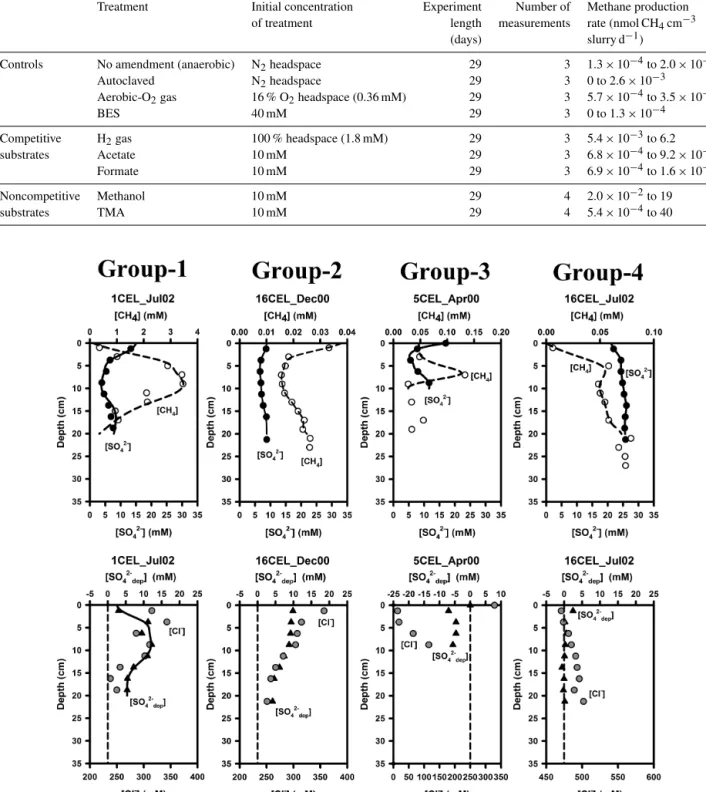
Table 1.Experimental conditions and sampling time intervals for methane headspace concentration analyses of sediment slurry incubations.

Treatment Initial concentration Experiment Number of Methane production of treatment length measurements rate (nmol CH₄cm⁻³

(days) slurry d⁻¹)

Controls No amendment (anaerobic) N2headspace 29 3 1.3×10⁻⁴to 2.0×10⁻³

Autoclaved N₂headspace 29 3 0 to 2.6×10⁻³

Aerobic-O₂gas 16 % O₂headspace (0.36 mM) 29 3 5.7×10⁻⁴to 3.5×10⁻³

BES 40 mM 29 3 0 to 1.3×10⁻⁴

Competitive H2gas 100 % headspace (1.8 mM) 29 3 5.4×10⁻³to 6.2

substrates Acetate 10 mM 29 3 6.8×10⁻⁴to 9.2×10⁻²

Formate 10 mM 29 3 6.9×10⁻⁴to 1.6×10⁻¹

Noncompetitive Methanol 10 mM 29 4 2.0×10⁻²to 19

substrates TMA 10 mM 29 4 5.4×10⁻⁴to 40

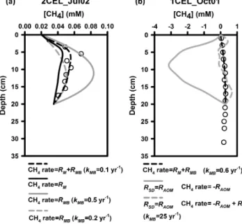
Figure 2.Depth profiles of modeled (lines), measured (circles) and calculated (triangles) concentration of dissolved methane (dashed lines;

open circles), sulfate (solid lines; solid circles) in the upper panel and sulfate depletion (solid lines; solid triangles), zero sulfate depletion (dashed lines) and chloride concentration (gray circles) in the lower panel for each profile type (Groups 1–4, see text). One selected profile per group is shown here for illustration and the other profiles for each group (9 cores for Group-1, 6 cores for Group-2, 2 cores for Group-3 and 3 cores for Group-4) are presented in the Appendix A (Fig. A1). CEL and CH represent cores collected from Celestún Lagoon and Chelem Lagoon.

(5)

tervals and at different substrate concentrations (Table 1). In- cubations consisted of three competitive substrates (H₂, acetate, formate), two non-competitive substrates (methanol, trimethylamine (TMA)), and four types of controls. The controls (preparation methods are described below) consisted of an un-amended sediment control under anaerobic conditions, an un-amended aerobic control (partial oxygen headspace), a killed control in which the sediment was autoclaved to kill all living organisms in the sediment, and a chemical control in which biological methanogenesis was inhibited through the addition of 2-bromoethanesulfonic acid (BES) to a final concentration of 40 mM within the slurry. Triplicate bottles were prepared for each condition (controls and substrate additions), and methane headspace concentrations were measured at 3–4 time intervals over the course of 29 days.

All the sediment slurries were prepared semi- anaerobically by homogenizing the sediment in a blender with an artificial seawater mixture in a 1:1 ratio under continuous flow of nitrogen gas. Large pieces of leaves, twigs, and shells were removed from the sediment prior to homogenization. 70 mL glass Wheaton bottles were flushed with nitrogen gas for 1 min prior to the addition of the sediment slurry. 30 mL of slurry was then added to each bottle under continuous nitrogen flow, and the bottles were sealed using blue butyl rubber stoppers and aluminum crimp seals. Substrate additions were made by injecting the substrate solution into the bottle immediately after sealing the bottles, except for the H2 gas treatment and the aerobic control. For the addition of H2, the entire headspace of the bottles was flushed with 100 % H2gas. After each headspace sampling the H2 gas removed by microbial activity in the sediment was replaced by inserting a gas tight syringe filled with 100 % H₂gas into the bottles, and allowing the gas to be drawn into the bottles until equilibrium pressure was reached. The aerobic controls were prepared like the anaerobic un-amended controls, except that 8 mL (20 % of the total headspace) of 100 % O₂ was added to the bottles immediately after they were sealed. In order to ensure that the sediment slurries remained aerobic, 100 % O₂was added to the bottles throughout the incubation period. The sediment slurries were kept at room temperate (22^◦C) and agitated continuously on a shaker table throughout the course of the incubations.

Headspace samples (0.25 mL) were extracted from the bottles at each time interval using a gas-tight syringe.

Methane concentrations were measured on an HP 5730A GC equipped with a flame ionization detector. GC calibration and creation of standard curves were based on successive dilu- tions of 100 % methane. Analytical error was approximately 5 % for methane concentrations below 10 ppm-v (446 nM), and less than 3 % for methane concentrations above 10 ppm- v as determined by repeat analyses of standards and samples.

4 Results

4.1 Porewater concentrations of dissolved species Representative porewater methane profiles were plotted alongside sulfate profiles in Figs. 2 and A1 in Appendix A.

Profiles were assigned to one of four profile types based on the relation between methane and sulfate distributions down core (see below). Considerable spatial and temporal variability in porewater chemistry was observed with no systematic seasonal differences in concentration trends. For example, porewater methane concentrations varied by up to 3 orders of magnitude in both lagoons, even between sites in close proximity to each other (i.e. 1CEL and 2CEL, Oct01; 1CH and 2CH, Dec00), and at the same station sampled during different seasons (i.e. 2CEL Dec00, Oct01; 1CH Apr00 and Oct01). No consistent differences were evident between the stations at the sides of the lagoons and those located in the center of the lagoons, or between stations located in the inner zone of the lagoons and those located near the mouth.

For instance, supersaturated methane concentrations of 1.1 and 1.3 mM were observed in cores 1CEL_Jul02 (the inner zone of Celestún lagoon) and 14CEL_Dec00 (near the mouth of Celestún lagoon), respectively. This is particularly interesting because the water column at the mouth of the lagoon has much higher salinities than the water of the inner zone (Young et al., 2008). The variability (both spatial and temporal) in the porewater methane concentrations and in profile types suggests a very dynamic system where both concentration and distribution patterns in the porewater vary con- stantly. Such variability is indicative of rapid methane production and efflux rates.

Porewater sulfate concentrations ranged from 0.21 to 35.3 mM in Celestún lagoon and from 4.13 to 33.5 mM in Chelem lagoon and showed different trends (Figs. 2, A1). In many of the cores a negative relation between methane and sulfate was observed. Specifically, higher sulfate was associated with lower methane in cores located near the mouth of the lagoons (16CEL_Jul02, 16CEL_Oct01, 14CEL_Oct01, 14CEL_Jul02 and 5CH_Apr00) and lower sulfate with high methane in the inner zone of the lagoons (e.g. cores 1CEL_Jul02, 1CEL_Dec00, 3CEL_Jul02, 3CEL_Apr00, 1_1CH_Oct01, and 1_2 CH_Oct01).

The relationship between porewater salinity (represented by chloride concentration), methane and sulfate concentrations was spatially and temporally variable (Fig. 3). Gen- erally, higher sulfate concentrations were associated with higher chloride in cores located near the mouth of the lagoons and lower sulfate with lower chloride in the inner zone of the lagoons (Fig. 3a). Despite these general trends there were no clear consistent relationships between methane and chloride (Fig. 3b) and sulfate and methane (Fig. 3c) when the data were considered collectively. The lack of consistent trends suggests multiple processes impacting the distribution of methane and sulfate. These include physical processes,

(6)

Figure 3.Relationship between(a)[Cl⁻] and [SO²⁻₄ ],(b)[Cl⁻] and [CH₄] and(c)[CH₄] and [SO²⁻₄ ] in porewater samples.

such as mixing and dilution by seawater or groundwater, and biological processes such as sulfate reduction, methanogenesis and methane oxidation. Brackish groundwater enters Ce- lestún lagoon through at least 30 subsurface discharge points (Young et al., 2008), and the chloride profiles suggest that some of this groundwater may seep through the sediments, resulting in localized decline in porewater salinities.

To account for mixing with seawater or freshwater and to extract information on the biological and chemical processes controlling the distribution of porewater solutes, the observed sulfate depletion ([SO²⁻₄

dep]_OBS)relative to seawater was calculated as the difference between the expected sulfate concentration contributed by seawater (based on porewater chloride concentration) and the measured sulfate concentration:

[SO²⁻₄

dep]_OBS=

[SO²⁻₄ ]_(SW)

[Cl⁻]_(SW) × [Cl⁻]_(measured)− [SO²⁻₄ ]_(measured) (1) where 0.05171 is taken as the^[SO

2−

4 ]_(SW)

[Cl⁻]_(SW) ratio (Pilson, 1998).

Positive values indicate that sulfate has been removed from the porewater, most likely through sulfate reduction, while negative values indicate an external source of sulfate not associated with chloride, in this case groundwater (see discussion below).

Based on the observed trends in sulfate depletion, when considered together with methane, four different porewater trends can be described, referred to as Groups 1 through 4 (Figs. 2, A1). The majority of profiles fell into Group-1 (ten cores); these profiles showed positive sulfate depletion profiles (e.g. sulfate consumption or loss) with methane profiles mirroring the sulfate concentration profiles (methane production or input). The peaks for methane and sulfate depletion occurred at the same depth as the lowest measured sulfate concentrations. In Group-2 (seven cores), sulfate depletion also showed positive values (sulfate consumption) but not throughout the core. In some cores sulfate depletion was close to zero at shallow depths and then increased with depth and in other cores positive sulfate depletion values appeared at the surface of the sediments and then decreased to almost zero at deeper depths. Methane concentrations for this group showed no clear relation to the sulfate profiles. In Group-3 (three cores), sulfate depletion showed negative values (e.g.

sulfate addition). The values became more negative toward the deeper sediment starting from zero right at the surface suggesting that sulfate was being added from the bottom of the sediment section. In Group-4 (four cores), there was almost no sulfate depletion (sulfate concentrations similar to seawater) from the surface to the deeper depths and methane concentrations were low (< 0.25 mM) increasing at depth, in- dicating a deeper source of methane.

4.2 Sediment slurry incubation experiments

All the sediment slurries with added substrates showed an increase in headspace methane concentration that was sig-

(7)

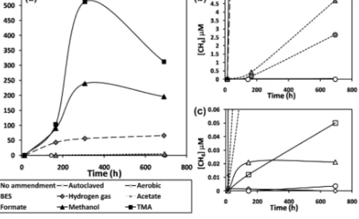
Figure 4. (a)Headspace methane concentrations in sediment slurry incubations.(b)Expansion of(a), showing results for acetate, formate, and controls.(c)Expansion of(a), showing results for controls only. Error bars represent 1 standard deviation for triplicate sample bottles.

nificantly greater than those observed with either the un- amended aerobic and anaerobic controls or the treated controls (Fig. 4). The greatest increases in headspace methane concentration were seen with additions of the two non- competitive substrates, TMA and methanol. The H₂ treatment showed the next highest methane production rate, followed by formate and acetate. Of the four control conditions, the un-amended, anaerobic treatment had the highest over- all increase in headspace methane concentration. The aerobic treatment had an initial higher increase in headspace methane concentration than the un-amended, anaerobic treatment, although there was no detectable change in the headspace methane concentration in the aerobic treatment between 150 and 700 h. Both the autoclaved and BES treatments did not show any changes in headspace methane concentration greater than the instrumental detection limits. The maximum methane production rates for each treatment are listed in Ta- ble 1.

5 Discussion

5.1 Co-existence of methane and sulfate in sediments Seawater transport into the sediment by diffusion and bioir- rigation due to the activity of burrowing animals has clear effects on porewater solutes. These processes are a source of seawater sulfate and mask sulfate loss by microbial reduction. Although, as indicated above, considerable variability in porewater profile distribution trends was observed, and different profile types were found throughout the lagoons, certain trends were more common at distinct locations. Specifically, sites characterized by sulfate addition from input of seawater into the sediment (cores in Group-4) were found primarily near the mouth of both lagoons where

low methane was associated with near-zero sulfate depletion. Negative sulfate depletion (Group-3), on the other hand, which indicates the presence of porewater that is enriched in sulfate relative to chloride, was seen primarily in the middle zone of Celestún Lagoon where groundwater springs rich in sulfate due to anhydrite dissolution are present, as reported by Perry et al. (2002, 2009). Positive sulfate depletion profiles co-occurring with methane (Groups 1 and 2) were seen throughout the lagoons but mostly at sites in the inner zone of both lagoons, suggesting significant sulfate reduction at rates higher than the replenishment from sulfate rich groundwater or from the overlying seawater and a source of methane to the shallow sections of the sediment.

It is surprising that at many sites, particularly within Groups 1 and 2 in the inner zone of both lagoons (1CEL, 2CEL, 3CEL and 1CH), high concentrations of methane and sulfate co-occurred at the same depth in the sediment.

Co-existence of methanogenesis and sulfate reduction is not normally observed because sulfate reduction is more ener- getically favorable than methanogenesis, and sulfate reducers should outcompete methanogens for common substrates such as hydrogen and acetate (Oremland and Polcin, 1982;

Jørgensen and Kasten, 2006). Moreover, anaerobic oxidation of methane (AOM) coupled with sulfate reduction at the base of the sulfate reducing zone should further deplete methane (Capone and Kiene, 1988; Valentine and Reeburgh, 2000). There are several possible explanations for these observations: firstly, the high methane concentrations measured in the sulfate rich porewater may be supplied by a rapid non-diffusive mechanism from below the sulfate reduction zone (like rising gas bubbles), limiting the exposure time to AOM. Secondly, methane may be produced in situ at these depths supported by a high abundance of competitive substrates in the sulfate reduction zone hence sustain- ing both methanogenesis and sulfate reduction (Holmer and Kristensen, 1994). Thirdly, methanogens may instead be able to thrive on various non-competitive substrates (Oremland and Polcin, 1982; Wellsbury and Parkes, 2000; Lee et al., 2008; Taketani et al., 2010). Indeed, use of non-competitive substrates by methanogens, including methanol, trimethy- lamines and dimethylsulfide, has been reported for mangrove sediments, coastal lagoons and continental shelf sediments (Ferdelman et al., 1997; Lyimo et al., 2000; Mohanraju et al., 1997; Purvaja and Ramesh, 2001; Torres-Alvarado et al., 2013; Maltby et al., 2016). Our slurry incubation experiments demonstrated that the methanogenic community at Celestún is capable of using a wide range of substrates, including H₂, acetate, formate, methanol, and trimethylamine (Fig. 4). Both methanol and trimethylamine are not utilized by sulfate reducers, which could allow methanogens to thrive in the sulfate reduction zone (Fig. 4). The use of non- competitive substrates by the methanogenic community has important implications for methane fluxes to the atmosphere as it allows for methane production at shallow depths in the sediment and reduces the potential for complete oxidation

(8)

of methane. Although processes and trends similar to those described above have been reported for other mangrove sediments (e.g., Lee et al., 2008; Purvaja and Ramesh, 2001), the co-occurrence of sulfate and methane and related bio- geochemical reactions in these reports remain qualitative in nature. In the following section, we use a transport-reaction model to better quantify the processes controlling methane fluxes from the sediments in these mangrove-dominated tropical coastal lagoons.

5.2 Model set-up and application to

mangrove-dominated coastal lagoon sediments In order to understand methane production and consumption and how these processes relate to sulfate dynamics in the lagoon sediments, we used two different approaches to simulate methane and sulfate porewater profiles.

In the first approach, a transport-reaction model was applied to profiles of Group-1 where methane and sulfate co- occur with no indication of groundwater sulfate input and where sulfate reduction surpasses sulfate addition from seawater (Figs. 2; A1). Data in Group-1 have positive net sulfate depletion rates indicative of sulfate reduction. The sulfate depletion is seen within the zone where methane concentrations are high. In these cores the net sulfate depletion rates can be used to derive the minimum methanogenesis rates (see model details in the Appendix A). Reactions considered in this first approach include organic matter degradation via heterotrophic sulfate reduction, methane production via methanogenesis and methane addition from gas bubble dissolution (Haeckel et al., 2004; Chuang et al., 2013).

A second approach (detailed in the Appendix A) was used for simulating the profiles for Group-2, Group-3 and Group- 4 which show no positive net sulfate depletion rates when integrated over the core length. These sites are affected by groundwater input or by considerable irrigation and input of seawater. Here, the link between sulfate and methane reactions is less clear and hard to quantify directly.

The following equation was solved to quantify the rates of reaction and transport of dissolved methane and sulfate in the upper 20 cm of the sediments in both approaches (Berner, 1980; Boudreau, 1997):

8·∂C

∂t =∂ 8·D_s·^∂C

∂x

∂x −∂ (8·v·C)

∂x +8·R_c, (2) where x is sediment depth, t is time, 8 is porosity, Ds is the solute-specific diffusion coefficient in the sediment,Cis the concentration of methane or sulfate in the porewater, v is the burial velocity of porewater andR_C is the sum of reactions affecting C (Table A1 in the Appendix A). Solutes were simulated in moles L⁻¹ of porewater (M). Details of all the reaction terms and parameters and how they were derived for each of the two approaches are given in the Ap- pendix A. The model assumes steady-state conditions to con- strain methanogenesis rates at each site. Considering the ob-

Figure 5.Model sensitivity analysis of methane concentrations for cores in Group-1 to the different processes controlling methane concentrations in porewaters. Black dashed lines denote the standard simulation results: CH₄production rate= +RMB+RM.RM is methanogenesis,R_MBis methane bubble dissolution,R_AOMis anaerobic oxidation of methane andR_SDis net sulfate depletion.

served variability in porewater distributions non-steady state simulations would be desirable, yet this would require continuous monitoring of porewater sulfate, methane and chloride concentrations to evaluate temporal changes in sulfate depletion at each site. These time series data are unavailable, hence the modeled “instantaneous” rates bear uncertainties that currently cannot be quantified accurately.

Model derived sulfate depletion and sulfate and methane concentrations are shown in Figs. 2 and A1. Modeled porewater data for Group-1 (the most common trend) show that methane generated from organic matter degradation within the upper sediments is a more important methane source than methane diffusing from below and gas bubble dissolution, as further seen in the results of 1CEL_Jul02 and the sensitivity analysis from 2CEL_Jul02 (Fig. 5a). In 1CEL_Jul02, for example, gas dissolution of methane transported from deeper sediments is not necessary at all to achieve a good model fit to the data, and in-situ methanogenesis alone can reproduce methane concentrations similar to the measured data even though methane concentrations are oversaturated (> 1.1 mM (in situ solubility); Fig. 2). In contrast, the modeled methane profile for 2CEL_Jul02 (black dashed line) ar- guably does require the inclusion of methane from gas dissolution (R_MB; Fig. 5a). In Fig. 5a, the gray dashed and solid lines represent only gas dissolution in the methane reaction terms (no methanogenesis within the modeled 20 cm column) using different gas dissolution constants (k_MBvalues are 0.2 and 0.5 yr⁻¹respectively). The model results shown

(9)

as the gray dashed line simulate the methane concentrations below 10 cm depth, whereas those shown by the gray solid line reproduce methane concentrations in the upper 5 cm, but neither reproduces the data throughout the whole core.

Comparing results considering methanogenesis and gas dissolution (black solid line) and methanogenesis only (black dashed line), it is clear that both methanogenesis and some gas dissolution are needed for reproducing the methane distribution observed in core 2CEL_Jul02. This illustrates the complexity of controlling processes and the dynamic nature and resulting temporal variability in methane fluxes at this and the other sites in the lagoons.

5.3 Model derived depth-integrated turnover rates and fluxes

Table 2 lists the calculated depth-integrated turnover rates and fluxes for the individual cores. For profiles in Group- 1, methane sources include methanogenesis within the upper 20 cm and/or methane transported from deeper sections (> 20 cm) via bubble transport and dissolution.

Methane can be supported fully by methanogenesis without gas bubble dissolution within the modeled upper 20 cm in cores 1CEL_Dec00, 1CEL_Jul02, 1_1CH_Oct01 and 1_2CH_Oct01. Gas bubble transport from deeper sediments and its dissolution contributes more methane than methanogenesis in cores 1CEL_Apr00, 1CEL_Oct01, 2CEL_Dec00 and 3CEL_Jul02.

Methane sinks include fluxes into the water column or methane diffusion into deeper sediments (> 20 cm) and methane oxidation. Our model shows that the major sink for methane is efflux to the water column accounting for over 90 % of methane produced within the upper 20 cm (e.g. 1CEL_Apr00, 1CEL_Oct01, 3CEL_ Apr00 and 3CEL_Jul02). Model-derived methane fluxes to the water column are listed in Table 2 (Fmethane (top)) and range from 0.012–20 mmol CH₄m⁻²d⁻¹. These rates are similar to or up to 2 orders of magnitude larger than fluxes reported for other mangrove lagoon systems in Florida (0.02 mmol CH₄m⁻²d⁻¹, Barber et al., 1988; Harriss et al., 1988), Australia (0.03–

0.52 mmol CH4m⁻²d⁻¹, Kreuzwieser et al., 2003), and India (5.4–20.3 mmol CH4m⁻²d⁻¹, Purvaja and Ramesh, 2001). Since all methane depth profile types were observed throughout the year with no obvious trends in spatial and temporal distribution (seasons and sampling locations), our results support the idea that methane fluxes in coastal mangrove lagoon systems respond very dynamically to environmental stimuli.

Sulfate sinks include heterotrophic sulfate reduction and AOM, although the model suggests that AOM plays a minor role compared to heterotrophic sulfate reduction. Sulfate reduction ranges from 1.1 to 24 mmol SO²⁻₄ m⁻²d⁻¹and is the major sink for both sulfate and organic carbon in most cores.

Sulfate reduction accounts for 2.2 to 48 mmol C m⁻²d⁻¹of

total anaerobic carbon respiration, which is in the same range of values listed in Kristensen et al. (2008) for other mangrove sediments.

Mangrove forests are known to be highly productive systems with the capacity to release high concentrations of dissolved organic matter (DOM) to surrounding sediments and porewaters (Kristensen et al., 2008). Tree litter and subsurface root growth provide further significant inputs of organic carbon to mangrove sediments which are unique for this type of system. The rate of organic matter mineralization (R_POC; Eq. A6 in the Appendix A) derived from sulfate depletion ranges from 3.2 to 110 mmol C m⁻²d⁻¹. Although our modeling approach for determining degradation rates is not without uncertainty, it is more accurate than rates derived from down-core trends in organic matter content because of temporal variability in accumulation rates in this area (Gonneea et al., 2004). Particulate organic matter will also contain a high amount of refractory carbon that is not easy to quantify and separate from the bulk pool. The derived degradation rates likely represent the more labile particulate components and labile DOM that was not considered (or measured) in this study. The high calculated organic carbon oxidation rates derived here are thus not unexpected since mangrove systems in general (e.g. Dittmar and Lara, 2001; Dittmar et al., 2006;

Lee, 1995; Odum and Heald, 1975) and the lagoons in Yu- catán in particular are dominated by high concentrations of DOM, a large fraction of which is likely to be labile (Young et al., 2005).

Depth-integrated methane production or consumption rates (RCH₄)and net sulfate inputs (R_SO2−

4 )calculated from Eqs. (A9) and (A10) for cores in Group-2, Group-3 and Group-4 are listed in Table 2. The methane and sulfate net production/consumption rates ranged from −0.060 to 11 mmol CH4m⁻²d⁻¹ and−69 to 21 mmol SO²⁻₄ m⁻²d⁻¹ (negative values indicate net sulfate or methane consump- tions while positive values indicate production or addition from external sources). Although sulfate depletion values for cores in Group-2 are positive (e.g. net sulfate reduction), sulfate concentrations at some depths of the porewater are relatively high, suggesting continuous sulfate input from deeper within the sediments or from seawater. Cores in Group-3 and Group-4 show negative or zero sulfate depletion that likely results from high rates of sulfate addition from groundwater (Group-3) or seawater (Group-4), thus prohibiting accurate calculation of sulfate reduction and methanogenesis rates. Although, in theory, H2S oxidation is a possible source for the excess sulfate, we believe that sulfate-rich groundwater input is a more likely source due to correlation between excess sulfate and excess Sr which has been previously described for groundwater in this region (Young et al., 2008).

Perry et al. (2002) identified dissolution of evaporites within the freshwater lens at some Yucatán sites as a probable source of excess sulfate in groundwater using the sulfate-to-chloride ratio (100×^[SO

2−

4 ]

[Cl⁻]). Ratios higher than seawater (average

(10)

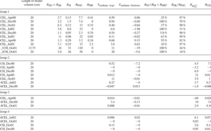
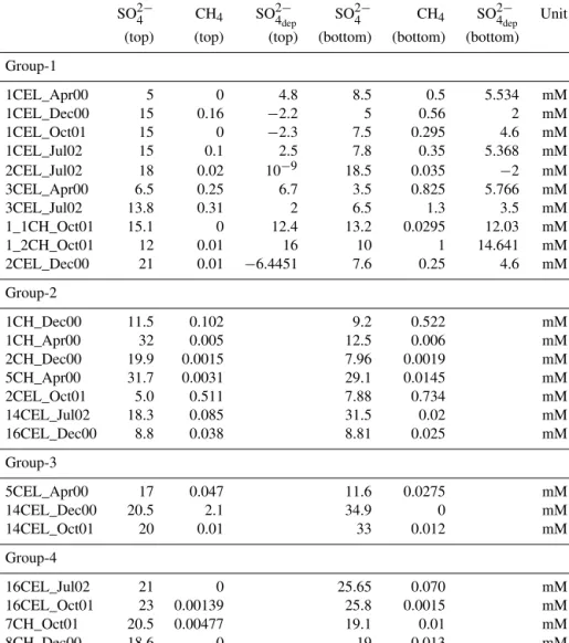
Table 2.Model-derived depth-integrated turnover rates (mmol m⁻²d⁻¹), dissolved methane fluxes to the water column (mmol m⁻²d⁻¹) and contributions of methanogenesis to net methane production (%) and heterotrophic sulfate reduction to POC degradation (%). CEL and CH represent cores collected from Celestún Lagoon and Chelem Lagoon.

Length of model

column (cm) R_SD=R_SR R_M R_POC R_MB Fmethane (top) Fmethane (bottom) R_M/(R_M+R_MB) R_SR/R_POC R_SO2−

4

R_CH₄

Group-1

1CEL_Apr00 20 3.7 0.13 7.7 0.41 0.59 0.06 25 % 97 %

1CEL_Dec00 20 2.2 1.5 7.4 0 0.94 −0.60 100 % 59 %

1CEL_Oct01 20 6.2 0.12 13 0.32 0.40 −0.04 27 % 98 %

1CEL_Jul02 20 3.6 8.0 23 0 6.0 −1.98 100 % 31 %

2CEL_Dec00 20 1.1 0.05 2.3 0.76 0.54 −0.27 5.8 % 96 %

2CEL_Jul02 20 11 0.08 22 0.05 0.11 −0.02 63 % 99 %

3CEL_Apr00 20 1.3 0.29 3.2 0.24 0.68 0.15 55 % 82 %

3CEL_Jul02 20 7.1 0.25 15 2.2 3.0 0.63 10 % 97 %

1_1CH_Oct01 13.75 24 31 110 0 11 −19 100 % 44 %

1_2CH_Oct01 20 3.0 26 58 0 20 −5.6 100 % 10 %

Group-2

1CH_Dec00 20 0.52 −7.2 4.5 7.8

1CH_Apr00 20 ∼0 ∼0 −3.2 ∼0

2CH_Dec00 20 ∼0 ∼0 6.9 ∼0

5CH_Apr00 20 0.012 ∼0 21 0.013

2CEL_Oct01 20 11 −0.01 3.9 11

14CEL_Jul02 20 0.27 ∼0 3.7 0.27

16CEL_Dec00 20 −0.047 0.013 −1.8 −0.060

Group-3

5CEL_Apr00 10 0.014 −0.01 −69 0.028

14CEL_Dec00 20 3.4 −0.13 10 3.6

14CEL_Oct01 20 0.088 −0.01 2.9 0.10

Group-4

16CEL_Jul02 20 0.096 0.02 6.1 0.072

16CEL_Oct01 20 ∼0 ∼0 0.83 ∼0

7CH_Oct01 20 0.13 ∼0 2.6 0.14

8CH_Dec00 20 ∼0 ∼0 0.85 0.012

R_SDis net sulfate depletion (mmol m⁻²d⁻¹of SO²⁻₄ ).R_SRis heterotrophic sulfate reduction (mmol m⁻²d⁻¹of SO²⁻₄ ).R_Mis methanogenesis (mmol m⁻²d⁻¹of CH₄).R_POCis total POC mineralization (mmol m⁻²d⁻¹ of C).RMBis gas dissolution (mmol m⁻²d⁻¹of CH₄).Fmethane(top)is the methane flux across the sediment surface (mmol m⁻²d⁻¹of CH₄). Negative values inFmethane(top)represent methane flux into the sediments from the water column and vice versa.Fmethane(bottom)is the methane flux across the 20 cm lower boundary (mmol m⁻²d⁻¹of CH4). Negative values inFmethane(bottom)represent methane flux to deep sediments and vice versa.

RSO2−

4

is net sulfate input (mmol m⁻²d⁻¹of SO²⁻₄ )andR_CH4is net methane production (mmol m⁻²d⁻¹of CH₄)for cores in Group-2 to Group-4. See Appendix A for further model details.

seawater is 10.3) are expected where gypsum/anhydrite dissolution occurs (Perry et al., 2002). Another indicator is the Sr/Cl ratio, which is invariably higher in the Yucatan groundwater than in seawater and indicates dissolution of ce- lestite (from evaporite) and/or aragonite (Perry et al., 2002).

The region east and south of Lake Chichancanab, referred to as the Evaporite Region by Perry et al. (2002), is characterized by distinctive topography and high sulfate groundwater concentrations (Perry et al., 2002). The groundwater from the Lake Chichancanab area flows northward into the Celestún Estuary which can be recognized by the progressive decrease in the ratio

[SO2−

4 ] [Cl− ]groundwater

[SO2−

4 ] [Cl− ]seawater

in water from southeast to north- west (Perry et al., 2009). Some groundwater samples with sulfate concentrations as high as 32 mM were reported in Young et al. (2008) and the Sr and sulfur trends for Celestún lagoon (Young et al., 2008) are consistent with our interpre- tation that gypsum/anhydrite dissolution in groundwater is the source of excess sulfate in the porewater of Group-3 in

Celestún lagoon. Due to the impact of groundwater, our sulfate reduction and methanogenesis rates estimated using the model are minimum rates and independent rates of groundwater discharge into each core are needed for obtaining more realistic estimates in these sites.

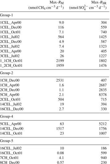
In addition to depth-integrated rates, Table 3 also includes maximum methanogenesis/methane production (Max-RM) and sulfate reduction/consumption (Max-R_SR)rates solved by Eq. (2) in the model. It is encouraging that the maximum methane production rates estimated from TMA, methanol and H₂ additions to sediments in the slurry incubations (Table 1) are similar to model-derived Max-R_M at station 16CEL (Table 3), which is the site from which sediments were collected for the slurry incubations. The rates in the TMA, methanol and H₂treatments from the slurry incubations (Table 1) and in some of our stations are higher than methane production rates from previously reported coastal freshwater and brackish wetland sediments that were measured using radiolabeled acetate and bicarbonate in slurries (Segarra et al., 2013).

(11)

Table 3.Maximum model-derived rates of methanogenesis and sulfate reduction for cores in Group-1 and maximum model-derived rates of methane production and sulfate consumption for cores in Group-2, Group-3 and Group-4. CEL and CH represent cores collected from Celestún Lagoon and Chelem Lagoon.

Max-R_M Max-R_SR

(nmol CH₄cm⁻³d⁻¹) (nmol SO²⁻₄ cm⁻³d⁻¹) Group-1

1CEL_Apr00 9.0 304

1CEL_Dec00 116 559

1CEL_Oct01 7.1 740

1CEL_Jul02 564 1425

2CEL_Dec00 4.9 587

2CEL_Jul02 7.4 1323

3CEL_Apr00 20 405

3CEL_Jul02 26 1227

1_1CH_Oct01 2199 1802

1_2CH_Oct01 1959 1476

Group-2

1CH_Dec00 2531 407

1CH_Apr00 1.6 2687

2CH_Dec00 1.1 2835

5CH_Apr00 2.1 8378

2CEL_Oct01 504 715

14CEL_Jul02 19 394

16CEL_Dec00 2.7 330

Group-4

5CEL_Apr00 63 5212

14CEL_Dec00 1517 1756

14CEL_Oct01 23 1007

Group-5

16CEL_Jul02 10 186

16CEL_Oct01 0.08 599

7CH_Oct01 4.1 940

8CH_Dec00 0.57 230

Modeled Max-R_M in some cores were 1–2 orders of magnitude higher than rates derived from the sediment slurry incubations (e.g., cores 1CEL_Jul02, 1_1CH_Oct01, 2CEL_Oct01 and 14CEL_Dec00). Although heterotrophic sulfate reduction generally dominates organic matter degradation, Max-RM values are even higher than the maximum sulfate reduction rates in some cores (1_1CH_Oct01, 1_2CH_Oct01 and 1CH_Dec00). Both the methanogenesis rates measured in the sediment slurry incubations and the modeled maximum methanogenesis rates in this study area were much higher than those reported for some mangrove systems (e.g., Thailand, Kristensen et al., 2000; Malaysia, Alongi et al., 2004; Australia, Kristensen and Alongi, 2006) but similar to other sites in India (Ramesh et al., 2007).

AOM is expected to play an important role in oxidizing methane in tropical porewaters with abundant methane and sulfate (Biswas et al., 2007). However, our model results and sensitivity analyses indicate that AOM is insufficient to pre-

vent methane from escaping to the bottom water, probably because of the abundant organic matter available for sulfate reducers to use instead of methane. In our sensitivity tests (using core 1CEL_Oct01 as an example), if AOM is allowed to be responsible for sulfate and methane consumption (no heterotrophic sulfate reduction and methanogenesis;

R_SD=R_AOM)then methane concentrations would decrease to negative values (gray solid lines in Fig. 5b), which is in- consistent with observations. Although based on our data it is not possible to accurately quantify methane oxidation by calculating the relative proportion of sulfate loss due to heterotrophic sulfate reduction and/or AOM, our model results suggest AOM plays a minor role in this setting. It is also possible to have high rates of methane production and also AOM in the sediments but this is not captured as methane loss because there is more production than depletion. In addition the formation of gas bubbles and short residence time in the sediment due to shallow formation depth, low gas dissolution and fast release all contribute to lowering the relative impact of AOM. Other studies such as Lee et al. (2008) also detected the co-existence of porewater sulfate and methane in dwarf red mangrove habitats (Twin Cays, Belize) and and in that setting, like our study site, it was not possible to spatially separate the methanogenesis and AOM zones. Future inves- tigations on the role of AOM in these dynamic mangrove- dominated tropical coastal lagoons are needed (e.g., Thalasso et al., 1997; Raghoebarsing et al., 2006; Lee et al., 2008;

Kristensen et al., 2008; Beal et al., 2009; Silvan et al., 2011;

Segarra et al., 2013).

6 Conclusions

The variable trends observed in sediment methane porewater chemistry from mangrove-dominated tropical coastal lagoons in Yucatán, Mexico, indicate a very dynamic system spatially and temporally throughout the year. This can be explained by multiple controlling parameters including physical processes such as mixing and dilution with seawater or groundwater, gas bubble rise and dissolution and microbial processes which operate at different rates during different times at all sites. Although our modeling suggests that organic carbon degradation rates are dominated by heterotrophic sulfate reduction in these cores, methanogenesis both in shallow and deeper sediments is also prevalent. The co-occurrence of methane and sulfate reduction (documented by sulfate depletion) in shallow sediments in this system is explained by high methane production rates supported by some combination of non-competitive substrates and ample dissolved and labile organic matter in the shallow sediments as well as the additions of methane from deeper sediment through gas rise and dissolution. Model results demonstrate that the largest sink for the methane in these sediments is efflux to the water column. Build-up of methane at shallow depths may reduce the fraction of methane that is oxidized

(12)

prior to entering the water column, thereby increasing the flux at the sediment-water interface. This shallow methane pool may also encourage methane flux through bubble release, which can result in a larger fraction of the methane reaching the atmosphere without being lost to oxidation.

Specifically, the ability of the microbial community in these sediments to use non-competitive substrates may allow for methane production in the upper sections of the sediment, po- tentially contributing to the higher than expected atmospheric methane flux measured from mangrove-dominated tropical coastal lagoons.

(13)

Appendix A: Modeling procedure used in the evaluation of porewater observations from sediments in

mangrove-dominated tropical coastal lagoons, Yucatán, Mexico

Details of the modeling procedure and parameters used are described here. The following reactions are considered in the model:

Heterotrophic sulfate reduction (R_SR):

2CH₂O+SO²⁻₄ →2HCO⁻₃ +H₂S (AR1) Methanogenesis (R_M):

2CH₂O→CO₂+CH₄ (AR2)

Gas bubble dissolution (RMB):

CH4(g)→CH4(aq) (AR3)

The net reaction terms (R_C in Eq. 2) are given in Table A1, boundary conditions are listed in Table A2, best-fit model parameters are given in Table A3 and model-derived concentration profiles are shown in Figs. 2 and A1.

In Eq. (2), sediment porosity decreases with depth due to steady-state compaction:

8=8_f+ 80−8_f

·e^−px, (A1)

where 8_f is the porosity below the depth of compaction (0.78 for Celestún and 0.83 for Chelem),8₀ is porosity at the sediment surface (0.90 for Celestún and 0.89 for Chelem) andp(1/15 cm⁻¹)is the depth attenuation coefficient. These parameters were determined from the measured porosity data at each site or at a nearby site (Eagle, 2002).

Under the assumption of steady-state compaction, the burial of porewater was calculated as in Berner (1980):

v=8_f ·w_f

8 , (A2)

wherewf is the sedimentation rate of compacted sediments calculated from excess²¹⁰Pb data (0.25 cm yr⁻¹for Celestún and 0.35 cm yr⁻¹ for Chelem; Gonneea et al., 2004). Sedi- ment burial results in the downward movement of both sediment particles and porewater relative to the sediment water interface.

The sediment diffusion coefficient of each solute (D_s) was calculated according to Archie’s law considering the effect of tortuosity on diffusion (Boudreau, 1997):

D_s=8²·D_M, (A3)

whereD_Mis the molecular diffusion coefficient at the in situ temperature, salinity and pressure (Table A1) calculated according to Boudreau (1997). We used the same tortuosity coefficient (8²corresponding tom=3 in Archie’s law) as reported by Wallmann et al. (2006) for fine-grained sediments.

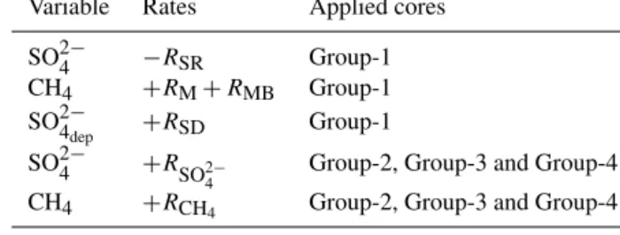
Table A1.Rate expressions applied in the differential equations (R_Cin Eq. 2).

Variable Rates Applied cores

SO²⁻₄ −R_SR Group-1

CH₄ +R_M+R_MB Group-1 SO²⁻₄

dep +R_SD Group-1

SO²⁻₄ +R

SO²⁻₄ Group-2, Group-3 and Group-4 CH₄ +R_CH₄ Group-2, Group-3 and Group-4

Since net sulfate consumption is observed in Group- 1 profiles (Figs. 2, A1), we used the following calculations to obtain net sulfate depletion rates (R_SD; mmol SO²⁻₄ cm⁻³yr⁻¹). RSD is proportional to the difference between modeled (C(SO²⁻₄

dep))and measured concentrations (C(SO²⁻₄

dep)OBS):

R_SD=k_SD· C

SO²⁻₄

dep

OBS

−C SO²⁻₄

dep

(A4) The corresponding kinetic constant is set to be high (k_SD≥100 yr⁻¹)to ensure that simulated concentrations are very close to measured values.R_SDimplicitly includesR_SR as well as anaerobic oxidation of methane (R_AOM):

CH₄+SO²⁻₄ →HCO⁻₃ +HS⁻+H₂O (AR4) The numerical modeling procedure outlined in Wallmann et al. (2006) is used as a basis to simulate the rate of sedimen- tary organic carbon degradation (R_POC)by sulfate reduction and methanogenesis. Since the measured organic matter content in both lagoons showed evidence for a change in deposi- tional pattern over time (Gonneea et al., 2004; Eagle, 2002), these measurements cannot be used for reliable organic matter degradation calculations. Hence,RSR(Eq. A5 below) was first calculated and then used to estimateRPOC(Eq. A6) and subsequently to deriveRM (Eq. A7). Here, we assume the three Reactions (R1), (R)2 and (R4) co-occur in the sulfate reduction zone such that the net reaction for methanogenesis and AOM (Reactions R2 and R4) is equal to carbon respiration by heterotrophic sulfate reduction (Reaction R1). In other words,R_SD=0.5R_POC.

To approximate the fraction ofR_POCdue toR_MandR_SR, a Michaelis–Menten kinetic limitation term is applied to Eqs. (A5)–(A7) (Wallmann et al., 2006):

R_SR=R_SD=0.5·R_POC·f_SO2−

4

(A5) R_POC= RSD

0.5·fC·f_SO2−

4

(A6) RM=0.5·RPOC·

1−f_SO2−

4

(A7) where f_SO2−

4

=

CSO2−

4

CSO2−

4

+K_SR is the Michaelis–Menten rate- limiting term for sulfate reduction.

(14)

Figure A1.

(15)

Figure A1.

At sites where methanogenesis was insufficient to simulate the measured methane data, methane was added as an external source by dissolution of gas bubbles (Chuang et al., 2013). Gas bubbles were observed in the field. The rate of dissolution of the gas bubbles (Reaction R3) rising through the sediment (CH_4(g)→CH₄)was also considered as (Haeckel et al., 2004)

RMB=kMB· LMB−CCH₄

if CH₄≤LMB, (A8) whereL_MB is the in situ methane gas solubility concentration calculated using the algorithm of Duan et al. (1992a, b) and the site-specific salinity, temperature and pressure.R_MB depends on the first-order rate constantkMB, which is a fit- ting parameter that lumps together gas dissolution in addition to diffusion of dissolved gas in the bubble tubes and walls.

Since sulfate depletion profile trends in Group-2, Group- 3 and Group-4 show evidence of groundwater or seawater input with no positive depth integrated net sulfate depletion rates, the second approach for determining net methane and sulfate reaction rates for porewater data in these three groups is summarized as

RCH₄=kCH₄· CCH_4OBS−CCH₄

, (A9)

R_SO2−

4

=k_SO2−

4

·

C_SO2−

4 OBS

−C_SO2−

4

(A10)

Net methane and sulfate reaction rates are set to be proportional to the difference between modeled (C_CH₄ andC_SO2−

4

) and measured concentrations (C_CH_4OBS andC_SO2−

4 OBS

). The corresponding kinetic constantsk_CH₄ andk_SO2−

4

are listed in Table A3.

Methane fluxes at the boundaries were calculated using the model as follows:

FCH₄(x)=8(x)·

v(x)·CCH₄−Ds·dC_CH₄(x) dx

, (A11) wherex=20 cm is the bottom of the simulated core andx=0 cm is the sediment–water interface.

Fixed concentrations were imposed for all solutes at the upper and lower boundaries to values measured at or near the sediment–water interface and at 20 cm. The method-of- lines was used to transfer the set of finite difference equations of the spatial derivatives of the coupled partial differential equations to the ordinary differential equation solver (NDSolve) in MATHEMATICA v. 7.0, using a grid spacing which increased from ca. 0.015 cm at the sediment surface to 0.38 cm at depth. Since most of the porewater profiles were fitted directly, only a few years of simulation time (5 years) was needed to achieve steady state. Mass balance was typically better than 99.9 %.

(16)

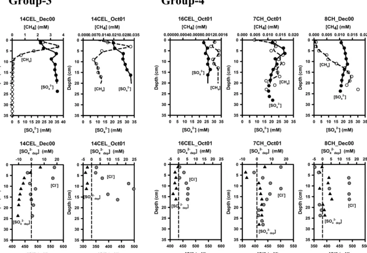
Figure A1.Depth profiles of modeled (lines), measured (circles) and calculated (triangles) concentration of dissolved methane (dashed lines;

open circles), sulfate (solid lines; solid circles) in the upper panel and sulfate depletion (solid lines; solid triangles), zero sulfate depletion (dashed lines) and chloride (gray circles) in the lower panel for each profile type (Groups 1–4, see text). One selected profile per group is shown in Fig. 2 for illustration and here the other profiles are shown (9 cores for Group-1, 6 cores for Group-2, 2 cores for Group-3 and 3 cores for Group-4). CEL and CH represent cores collected from Celestún Lagoon and Chelem Lagoon.