A STATE SPACE MODEL FOR BERLIN HOUSE PRICES ∗
Rainer Schulz
Ph.D. Program “Applied Microeconomics”
Humboldt-Universit¨at zu Berlin, Freie Universit¨at Berlin SFB 373, Humboldt-Universit¨at zu Berlin
Axel Werwatz
Institute for Statistics and Econometrics Department of Economics
Humboldt-Universit¨at zu Berlin August 2001
Abstract
How risky are investments in residential real estate? To answer this question, information is needed about the behavior of house prices.
The hedonic methodology has become a standard approach for mod- elling the prices of heterogeneous assets. Although intuitively appeal- ing, it is often criticized that this approach has no sound theoretical background. We have developed a model that partly circumvents this criticism. Based on an approximation for the present value, our model delivers a state space form for the determination of house prices. Thus,
∗ We would like to thank H. Herwatz and S.J. Koopman for helpful comments, the Gutachterausschuß f¨ur Grundst¨uckswerte in Berlin for providing us the data and for fruit- ful discussions. In addition, the first author would like to thank S.G. Athanasoulis, H.
L¨utkepohl, R.J. Shiller, and J. Wolters. Financial support from the Deutsche Forschungs- gemeinschaft, SFB 373 is gratefully acknowledged.
we can incorporate in an economically meaningful way other economic variables like the inflation rate, mortgage rates and returns of other assets. Under some restrictive conditions, our model reduces to the standard hedonic approach. We use the EM algorithm with a final scoring step to estimate our model with monthly data of single-family house sales from the four South-West districts of Berlin for the years 1982:7 to 1999:12.
JEL Codes: C32, C43, G12
Keywords: Present value, Hedonics, Kalman Filter, EM Algorithm, Model Selection, Cross-Validation Criterion
1 Introduction
In most industrial countries real estate is the greatest component of private household’s wealth. For example, in Germany real estate’s share of total wealth is about 53% (Deutsche Bundesbank 1999, p.43). For many house- holds, owner-occupied housing is the single most important asset in their portfolios. As a consequence, private households’ real estate investments are at center stage in the ongoing discussion about private pension schemes and optimal portfolio composition. Questions arising in this discussion are: How risky are investments in residential real estate? How is this risk related to the risk of other assets like stocks and bonds? Does real estate provide a hedge against inflation? Potential house buyers, sellers and developers of new houses are all interested in answers to these questions. Also banks want to know more about the risk of real estate because they use houses as collat- eral for mortgages. To answer these questions, a careful analysis of the time series properties of real estate prices is needed.
In this paper, we study the movement of house prices in Berlin, Germany, during a twenty year span. Our primary data source is a data base consisting of all transactions of single-family homes in Berlin between January 1980 and December 1999. Studying the development of house prices, though, is complicated by the fact that houses are heterogeneous assets. Indeed, it has been said that no two houses are ever identical. It is thus imperative in the empirical model to include variables that measure house characteristics. We
therefore make ample use of the rich information in our data set describing the properties of each unit sold.
The standard approach for constructing a model of the prices of hetero- geneous assets is hedonic regression (e.g. Shiller 1993, Cho 1996, Sheppard 1997, Hill, Knight, and Sirmans 1997). Due to the fact that the so-called repeat-sales approach derives from the hedonic methodology, we incorporate it under this heading (Dombrow, Knight, and Sirmans 1997). A hedonic model starts with the assumption that on average the observed price can be explained by some function f(It,xn,t,βt). Here, It is a common price component that “drives” the prices of all houses, the vector xn,t comprises the characteristics of house n and the vector βt contains all—possible time variable—coefficients of the functional form. Most studies assume a log-log functional form and that Itis just a period specific constant term. However, although there is some theoretical work on the derivation of functional forms (see the seminal paper of Rosen 1974), it is sometimes difficult to interpret the hedonic coefficients in a plausible way. We build on this work but go beyond the conventional specification in several important respects.
In our paper, we propose the well-known present value relation as a means to explain the behavior of house prices. Our approach is quite similar to the one used in Engle, Lilien, and Watson (1985). We generalize their approach.
First, we derive a hedonic regression equation from the well-known present value model of asset prices, thus providing theoretical motivation and aiding interpretation of the hedonic model. Still, present value theory does not ex- actly pin down the functional form of the hedonic regression equation. We therefore use a cross-validation criterion to choose between various possi- ble transformations of the continuous explanatory variables in the empirical work. Moreover we augment the hedonic equation by a model of the un- observable component of house prices reflecting the general tendency of the market for residential real estate. This component is assumed to be common to all prices in a certain period after controlling for the heterogeneity of house attributes. It is specified as an autoregressive process that also depends on financial variables such as the spreads between mortgage and interest rates with the same maturity or the returns of other assets such as stocks and
bonds. Our economic model associates this component of house prices with (expected) deviations from the long run rate of return of single-family homes.
The key to handling an hedonic model that has been augmented by an equation with an unobservable dependent variable is to write the model in state space form. Once the model has been put into this form, the Kalman filter can be used to estimate the unobservable price component and the EM algorithm can be used to calculate maximum likelihood estimates of the unknown coefficients of the model. Finally, we perform a scoring step to improve the efficiency of the EM algorithm estimates and to obtain estimated standard errors.
We estimate the augmented hedonic model using a subsample of the data base of all transactions that contains 4410 sales of single-family houses in the four South-West districts of Berlin between July 1982 and December 1999.
Our estimates of the coefficients of the hedonic equation provide plausible and easily interpretable values of the premiums or rebates that different house characteristics command. The estimated process of the common price component is highly persistent and sluggish.
The remainder of this paper is organized as follows: we motivate and derive a hedonic regression model in Section 2 with the help of present value theory. Because the present value formulae are highly non-linear, we use a well-known approximation. We also propose an equation for the unobservable price component. In the following section the empirical model is put into state space form and the estimation strategy is laid out. It basically consists of combining the Kalman filter and the EM algorithm to get estimates of the unknowns in our model. Section 4 contains the empirical part of the paper.
Section 5 interprets the results. The last Section concludes. An Appendix contains some derivations of used expressions.
2 Present Value Relation
We start with the assumption that the sales price of a house is equal to the sum of the discounted net proceeds that the investor expects in the
future. The economic reasoning for the relation is as follows: the buyer of a house accrues a “dividend” from holding the house whereas the seller incurs opportunity costs of not receiving this “dividend”. The dividend is simply the rent of the object. The process of the rent gives the cost of “shelter”.
This process must be discounted with a rate that compensates for the risk of holding a house. The discount rate is identical to the marginal return of other investments with the same level of risk. Due to this fact, we use “discount rate” and “return rate” as synonyms. That is the standard framework of the well-known present value relation (see Cochrane 2001)
Pn,t = X∞
j=1
Et
"
Dn,t+j
Qj
i=1(1 +Rt+i)
#
. (1)
HerePn,t denotes the sales price of housen that is sold in period t. Et[·] is a shorthand notation for the expectation taken conditional on the information available at time t. The net proceeds are given by the net rents Dn,t for the house. Given the gross rents, one can derive the net rents by accounting for maintenance and running costs. The net rents are discounted with time- varying rates Rt+j. Due to the last assumption, the above stated relation can be seen as a pure identity. Later on, we have to put structure on the process of the discount rate.
Instead of working with equation (1) directly, we use a log-linearized version of it (cf. Campbell, Lo, and MacKinlay 1997, Cochrane 2001). Let rt denote the log of one plus the return rate and dn,t the log rent. The first order approximation for the log price is
pn,t = k
1−ρ +dn,t+ X∞
j=0
ρj
Et[∆dn,t+1+j]−Et[rt+1+j]
(2) with ρ≡ 1/(1 +θ), k ≡ ln (1 +θ)−θlnθ/(1 +θ). Here, θ is the geometric average of the rent-price ratio during the sample period. We haveθ > 0 and ρ < 1. It is easy to see from (2) that ρ can be interpreted as a discount factor. The discount rate is given by θ. As usual, ∆ denotes the difference operator. So, ∆dn,t gives approximately the growth rate of the rents.
Under the assumptions of the well known Gordon growth model (cf.
Campbell, Lo, and MacKinlay 1997, p.256) the approximation of the log
price is exact. The assumptions of this model are that the discount rate and the growth rate of the expected rents are constant. Thus, (1) boils down to
Pn,t = (1 +G)Dn,t
R−G (3)
with the rent growth rate G and the discount rate R. With the constant rent-price ratio θ= (R−G)/(1 +G) we obtain
pn,t =dn,t−lnθ . (4)
It is easy to check that (2) reduces to this equation with rt+1+j = ln (1 +R) and ∆dn,t+1+j = ln (1 +G). Here, θ is the inverse of the so-called capital- ization rate. To derive the price one merely needs to capitalize—that is: to multiply—the rent with this rate.
Because we have data on owner-occupied houses it is impossible for us to observe the rents for the different objects. However, we have data on the rent index for Berlin. We will refer to the notional object that corresponds to this index as reference house. Let d0t denote this rent index. We assume that there exists a close connection between the unobservable rents of house n and the rent for the reference house. This connection is given by
dn,t=δ+d0t + (xn,t−x0)Tβ+εn,t (5) where εn,t is white noise. The constant δ absorbs the normalization of the rent index. xcomprises the—possibly transformed—characteristics for every object such as its age or its floor size. The characteristics of the reference dwelling, x0, are unobservable whereas the characteristics of house n, xn,t, are observable. The rent for housenis thus given by the rent for the reference dwelling plus a premium for differences in characteristics. The differences are evaluated with the implicit pricesβ. If we assume that the differences remain constant over time or that the characteristics switch to the characteristics of the reference object immediately after the sale we obtain with (5)
Et[∆dn,t+j] = Et[∆d0t+j] for j >0. (6) The assumption that the differences in characteristics remain constant is problematic if the reference object does not age. In that case, the valuation
coefficient for the age appears as a constant in (6). An example for a switch in characteristics is easily given: the house is vacant at the date of sale but the reference house is an occupied one. However, immediately after the sale the new owner will move in.
We derive now for (2) with (5) and (6) pn,t =κ+p0t −
X∞ j=0
ρjEt[rt+1+j] +xTn,tβ+εn,t (7) where κ absorbs all constants. Here,
p0t ≡d0t + X∞
j=0
ρjEt[∆d0t+1+j] (8)
is up to a constant equal to the fundamental value of the reference house.
This value would equal the price if the return rate deviation is zero. As such, it is just the sum of expected future rents, discounted at a constant rate. With a slight abuse of terminology, we will designate p0t directly as fundamental value.
To make the model empirically applicable we need to find expressions for the unobservable conditional expectations in expression (8). We propose that the growth rate of the rent can be modelled with a VAR(1) that incorporates lagged growth rates of the rent and perhaps other variables (building activity, income development etc.). Letvtcontain at least the current and some lagged observations of the rent growth rate. Then we have
vt+1 =c+Avt+ut+1 , (9) where c and A contain unknown coefficients, and ut+1 is noise. The first element invtis the current observation of the rent growth rate. Thus we get with the unit vector e1T = [1 0 · · · 0]
Et
∆d0t+1+j
=eT1 j
X
i=0
Ai
!
c+eT1Aj+1vt for j >0. (10) If the roots of ρA are inside the unit circle we obtain
X∞ j=0
ρjEt
∆d0t+1+j
= 1
1−ρeT1(I−ρA)−1c+eT1A(I−ρA)−1vt. (11)
The expression for the constant term is derived in Appendix A.1. To replace A and c, we estimate (9) for the whole sample period. After that, we are able to calculate the value of the discounted expected rent growth rates.
Thus far we have not considered the pure benefit of being the owner of a house. We have only controlled for the the differences in characteristics with respect to the reference house. It can be argued that house-ownership generates “value” per se, because it gives the owner the right to model the object in accordance to her own taste. But ownership also means incurring costs like transaction or property taxes. Furthermore, if the house is rented out the owner has to expend maintenance cost. In addition to that, there exists a principal agent problem between lessor and lessee. The unobservable renter will handle the dwelling with less care than the owner. However, the lessor commands a remuneration for this adverse effect and this will increase the rent relative to the notional rent for owner occupied housing (Homburg 1993). If all those influences remain constant during our sample period, they are captured in the constant κ. But, if they change during the sample period—for example, because of changes in tax rates—we have to control for them explicitly. Furthermore, there might be unusual circumstances—
e.g. personal relationship between buyer and seller, annuity payments—that influence the price. We will consider such changes and unusual circumstances explicitly through dummy variables in the vectors xn,t.
Finally, we must make assumptions about the behavior of the unobserv- able return rate rt. One possible specification for the process of the return rate is
rt+1+j =φrt+j + (1−φ)r∗+sTt+jγ+νt+1+j . (12) The random component νt is white noise. The required return depends on its own lagged values and on the long run rate r∗. Furthermore, the return is influenced by shocks st of some financial indicators. These indicators are spreads between mortgage and interest rates, the inflation rate, changes in interest or tax rates, and returns of stock indexes. We assume that these shocks are incorporated immediately into the return rate and thus Et[st+j] =
0 for j >0. We obtain after some manipulations
Et[rt+1+j] =r∗+φjEt[rt+1−r∗] for j >0. (13) It is easy to see that the long run required rate is equal to r∗ for |φ| <1. If we substitute (13) into the present value (7), define ret+1 ≡Et[rt+1−r∗] and assume |φ|<1/ρwe get (where—once again—all constants are absorbed by κ)
pn,t=κ+p0t − 1
1−ρφrt+1e +xTn,tβ+εn,t . (14) The expected changes in the return rate, re, are unobservable. However, rewriting (12) in deviation form forj = 0, taking expectations att and using rt−r∗ =ret +νt, we derive
ret+1=φrte+sTtγ+ ˜νt (15) with ˜νt≡φνt.
Letψ denote 1/(1−ρφ) and multiply the above equation with this term, one obtains eventually
∆0pn,t =κ−rψ,t+1e +xTn,tβ+εn,t . (16a) and
reψ,t+1 =φrψ,te +sTtγψ + ˜νψ,t (16b) Here, ∆0pn,tdenotespn,t−p0t. The subscript in the return equation indicates the transformation. The first equation is easy to interpret: the deviation between the current price and the fundamental price for the reference house is a linear function of the characteristics of the object, and the cumulative effect of the current return rate deviation. The second equation shows that the cumulated return deviations are influenced by their previous value and the shocks in the financial indicators. Because reψ,t is unobservable, we can not use OLS to estimate the price equation. However by writing down the system (16) as a state space model, we can apply the Kalman filter to estimate rψ,te .
3 State Space Form and Estimation Algorithm
The general state space form (SSF) is given as (withstate andmeasurement) αt=Ttαt−1+εst (17a)
yt=Ztαt+εmt . (17b)
withεst ∼ N(0,Rt) andεmt ∼ N(0,Ht) (this notation mainly follows Harvey 1989). The disturbance vectors are distributed independently.
If the disturbance terms in (16) satisfy the above stated distributional assumptions our model is easily arranged into SSF. LetNtdenote the number of all houses sold at timet. There areKβ house characteristics, andKγ short run influence variables. K = Kβ +Kγ + 1 is the number of constant state variables and S =K+ 1 is the number of all state variables. We obtain
αt ≡
rψ,t+1e
γ κ β
, Tt≡
"
φ sTt 01×(Kβ+1)
0K×1 IK
#
, εst ≡
"
˜ νψ,t
0K×1
#
(18a)
yt ≡
∆0p1,t
...
∆0pNt,t
, Zt≡h
−iNt 0Nt×Kγ iNt Xt
i , εmt ≡
ε1,t
... εNt,t
. (18b) Thus, whereas the number of state variables per period is equal to S and fixed, the number of observations per period—i.e. Nt—varies.
We are primarily interested in calculating the unobserved state vectors αt. They contain the cumulated discount rate deviations reψ,t+1, the coeffi- cients of the financial indicators γ, and the influences of the characteristics β. If we knew all parameters of the SSF (17), we could use the Kalman smoother to figure out the state vectors. On the other hand if we knew αt
the parameters could be readily estimated by maximum likelihood. In our model the variances of the disturbances and φ are unknown. To estimate
these coefficients we use the EM algorithm (Dempster, Laird, and Rubin 1977) and one subsequent step of scoring.
There is a vast literature about both methods and about some efficient ways to combine both methods (cf. Engle and Watson 1983). Normally, one should start with the EM algorithm and iterate until the parameter es- timates converge. After this is done, these estimates can be used as starting values for the scoring algorithm. This algorithm delivers as a by-product an estimate of the information matrix. Both algorithms start with the log- likelihood function of the state space form (17) and make extensive use of the Kalman filter and the Kalman smoother. The filter equations are given in Appendix A.2. However, we need some start values to initialize the esti- mation algorithm. We use OLS for this task. Furthermore, we carry out the necessary model selection for the rent equation (5) in the OLS framework.
In the next Subsection we discussion the estimation algorithm for the SSF.
Subsection 3.2 presents our model selection procedure.
3.1 The Estimation Algorithm for the SSF
To set up the log-likelihood we multiply the system of the state equations with theS dimensional unit vectore1. The log-likelihood is, up to a constant (cf. Wu, Pai, and Hosking 1996)
lnL(ψ) =− 1
2ln|Σ| − 1
2εT0Σ−1ε0
− 1 2
XT t=1
ln|R˜t| − 1 2
XT t=1
˜
εsTt R˜−t1ε˜st
− 1 2
XT t=1
ln|Ht| −1 2
XT t=1
εmTt H−t1εmt
(19)
with ε0 =α0−µ, ˜Rt ≡eT1Rte1, ˜εst =eT1(αt−Ttαt−1) andεmt =yt−Ztαt. However, we do not observe the state vectors. The idea of the EM algorithm is to maximize instead the expected value of the log-likelihood function. To derive the expected value of (19), let us define for t 6T
at|T ≡ET[αt] (20a)
Pt|T ≡ET[(αt−at|T)(αt−at|T)T] (20b)
Pt,t−1|T ≡ET[(αt−at|T)(αt−1−at−1|T)T]. (20c) Furthermore we rewrite
ε0 = (α0−a0|T) + (a0|T −µ),
˜
εst =eT1
(αt−at|T)−Tt(αt−1−at−1|T) + (at|T −Ttat−1|T) and
εmt = (yt−Ztat|T) +Zt(αt−at|T).
We have for our model Ht =σε2INt and ˜Rt=σ2˜νψ. The assumption of uncor- related errors in the discount rate and the price equation allows identification of the two variances (see Schwann 1998). After all, we obtain for (19) with E[εTΩ−1ε] = tr{Ω−1E[εεT]}
ET[lnL(ψ)] =− 1
2ln|Σ| − 1 2tr
Σ−1(P0|T + (a0|T −µ)(a0|T −µ)T)
− T
2 lnσ2˜ν− 1 2σν2˜
XT t=1
eT1Ste1− 1 2lnσε2
XT t=1
Nt
− 1 2σε2
XT t=1
tr{Mt}
(21)
where
St ≡ET[εstεsTt ] =Pt|T −Pt,t−1|TTTt −TtPt,t−1|T +TtPt−1|TTTt + (at|T −Ttat−1|T)(at|T −Ttat−1|T)T
and
Mt ≡ET[εmt εmTt ] =ZtPt|TZTt + (yt−Ztat|T)(yt−Ztat|T)T .
Due to the fact that the number of houses sold per period varies through time the filter procedure has to handle missing values. Generally, the Kalman
filter is well suited for handling missing observations (e.g. Harvey 1989, p.
144). One can either replace the missing observations with zeros and adjust the covariance matrix accordingly (see Shumway and Stoffer 2000, 4.4) or one can cancel out the missing observations from all matrices (Koopman, Shephard, and Doornik 1999). It is possible to show that both methods deliver equivalent results. We use the second method in our algorithms.
The unknown parameters—collected inψ—are µ, vechΣ, φ, σ2ε and σν2˜ψ. We have to choose these parameters in such a manner that the value of the expected log-likelihood is maximized. It is easy to see that ˆµ=a0|T and that there is no way to derive an optimal choice vech ˆΣ. So we use the covariance matrix derived for the OLS estimates. For the other unknown coefficients we obtain with the help of the first order conditions
ˆ
σν2˜ψ = 1 T
XT t=1
eT1Ste1 (22a)
ˆ
σ2ε = 1 PT
t=1Nt
XT t=1
tr{Mt} (22b)
φˆ= PT
t=1eT1(Pt,t−1|T +at|TaTt|T −Tt,−φ(Pt−1|T +at−1|TaTt−1|T))e1
PT
t=1eT1(Pt−1|T +at−1|TaTt−1|T)e1 , (22c) where Tt,−φ is Tt, but φ is replaced by a zero. The derivation of the last expression is given in Appendix A.3. The EM algorithm consists of the follow- ing iterative procedure: start with some reasonable values for the unknown coefficients (see Subsection 3.2), evaluate the matrices in the expected log- likelihood function with the Kalman smoother, and estimate the unknown coefficients. Use these estimates for a new evaluation of the expected log- likelihood and so on. Our algorithm stops if the relative change of the log- likelihood is below some prescribed convergence level. As Harvey (1989, p. 126) shows, it is possible to rewrite the log-likelihood (19) function in the prediction error decomposition form
lnL(ψ) =−1 2
XT t=1
ln|Ft| − 1 2
XT t=1
vTtF−t1vt (23)
with vt≡yt−Ztat|t−1. The matrixFt is a by-product of the Kalman filter.
In the above log-likelihood function we have omitted the expression fort = 0 and a constant term that depends solely on the number of observations.
The EM algorithm guarantees that the value of the likelihood increases for every iteration. However, it is a drawback of the algorithm that it does not deliver an estimate of the information matrix. This matrix is necessary to calculate standard errors for the estimated coefficients. Thus, we complete the estimation procedure with a final scoring step for (23) evaluated at the estimates of the EM algorithm. As Engle and Watson (1981) have shown, the elements of the information matrices are given by (with i, j = 1, . . .3)
Iij = XT
t=1
1 2tr
F−t1∂Ft
∂ψi
F−t1∂Ft
∂ψj
+
∂vt
∂ψi
T
F−t1∂vt
∂ψj
!
. (24) The derivatives are evaluated numerically with forward differences in the following way (see Fletcher 1987, p.23): run the filter with the estimated coefficients of the EM algorithm. Then rerun the filter three times, where in every pass one of the coefficients is perturbed slightly. We label such a pass for coefficient i with the superscript (i). For example, assume that the change of every coefficient is given by δ% (that is, ψ(i)i = (1 +δ)ψi). Then one obtains
∂Ft
∂ψi ≈(δψi)−1
F(i)t −Ft
and ∂vt
∂ψi ≈(δψi)−1
v(i)t −vt
. (25)
3.2 Model Selection and Initial Values
Economic theory does not suggest a particular functional form for the depen- dency of the rent on the explanatory characteristics of the respective house.
Most variables in (5) are dummies representing various qualitative charac- teristics of the houses such as their location or the presence of a swimming pool. These discrete explanatory variables naturally enter the model in a linear way. For the continuous variables the following Box-Cox type trans- formations are considered
Tλ(x) =
λ−1n
s−1(xλ+aλ)λ
−1o
for λ∈Λ, ln{s−1(x+a0)} for λ= 0
(26)
with Λ ={−2,−1,−0.5,0.5,1,2}. Here x denotes any of the continuous ex- planatory variables,aλ is a constant depending onλ,sis the sample standard deviation of variable xand λ is the parameter that determines the transfor- mation. A particular value of λ implies a value of the constant aλ. These constants are computed according to the suggestions made in Bunke, Droge, and Polzehl (1999) and aim to make, for any given λ, the transformation as nonlinear as possible.
If we rewrite the price equation (16a) withIt+1 ≡κ−rψ,t+1e we obtain
∆0pn,t =It+1+xTitβ+εit . (27) We choose λj for each of the J variables simultaneously by the following cross-validation criterion
λ∗ = arg min
XT t=1
Nt
X
n=1
∆0pn,t−∆\0p−n,t(λ)2
, (28)
where λ is the vector comprised of the λj for the different variables. Here,
∆\0p−n,t(λ) denotes the predicted value of ∆0pn,t from an OLS fit of regres- sion (27) using the transformations of the continuous explanatory variables according to the value of λ under consideration but omitting the observa- tion indexed (n, t) from the regression fit. By omitting an observation from the regression used for predicting that very observation the cross validated choice of λ∗ is optimal in the sense of minimizing an estimate of the ex- pected squared prediction error (see Bunke, Sommerfeld, and Stehle 1997, Bunke 1998). Given the best transformations, we can estimate the series for It, β, σε2 with OLS and use them and their covariances for the initializa- tion of our estimation algorithm. Furthermore, we can regress ˆIt+1 on own lagged realizations and other financial indicators to derive start values of the unknown coefficients of the discount rate equation.
4 Data and Estimation
The data sets are provided by the Gutachterausschuß f¨ur Grundst¨uckswerte in Berlin. This commission collects information on all real estate transac- tions in Berlin. The main data set contains about 22000 observations of
all transactions of single-family houses in Berlin between January 1980 and December 1999. Besides the price, we observe about 100 characteristics of each house such as the size of the lot, floor space, age of the house, location, availability and numerous qualitative variables indicating specific conditions of the house, the neighborhood or the transaction (e.g. transaction between relatives). We also have data for 5065 sales of apartment houses for the years 1980 to 2000. For every sold object we know the price and the yearly rent of the object. We use these data to calculate a proxy for the discount factor ρ that is used in the approximation (2) of the present value.
Before we characterize the sample we use for estimation, we want to give a brief description about Berlin’s market for real estate. According to the fig- ures of Berlin’s bureau of statistics (Statistisches Landesamt Berlin, StaLa), Berlin had 1.82 million dwellings in 1998. Here, dwellings comprise apart- ments, single family houses—detached, semi-detached, and row houses—, and condominiums. 11.04% of all non-vacant dwellings were privately owned.
The ratio between the floor space of the privately owned dwellings and rented dwellings was 1.55, where the average floor space for a rented apartment was 66.6 square meters in 1998. About 71% of all privately owned dwellings were condominiums (Statistisches Landesamt Berlin 1999).
For the estimation of our model, we take the observations of the four South-West districts Zehlendorf, Wilmersdorf, Steglitz, and Charlottenburg.
These districts cover 19% of Berlin’s area. In 1998 they accounted for 17%
of Berlin’s total population of about 3.4 million. The ratio of inhabitants to area lies a little bit above the average for all districts, but is much lower than the ratio for the inner city districts. 20% of all Berlin dwellings lay in the four South-West districts. 15% of the dwellings there—that is an absolute number of 48 600 dwellings—were privately owned. The average floor space in 1998 was about 81 square meters and was thus 15% higher than the average for the whole city. The unemployment rate in these districts is lower than the average for the whole city. All four districts are of high- quality and relatively homogeneous. Especially Wilmersdorf (Grunewald) and Zehlendorf (Wannsee) have very nice sections with forests and lakes. It is quite reasonable that houses in these districts share the same market risk,
so that yields of house ownership will be discounted by the same rate.
We measure the rent of the reference house,d0t,by the monthly rent sub- aggregate of the consumer price index for Berlin, provided by the StaLa.
However, the construction principle of this index changed slightly in the year 1995. All values of this index before 1995 are calculated for four person house- holds with middle income living in the Western part of Berlin. Thereafter, the values are calculated for all households. We assume, that this change does not influences the rent index as a measure of the opportunity cost.
Furthermore, in our model some information is not specific to the house but rather describe the opportunities of the investor. We have collected information about tax rates and government housing programs during the relevant time period. As financial indicators we have different monthly mort- gages rates (with varying degrees of interest rate fixedness), the range of these rates offered by different banks, the monthly consumer price index for Berlin West, monthly interest rates given by returns on bonds, the return of the DAX stock index (a performance index) and the return of the CDAX stock index (a price index). The different mortgage rates and the ranges are avail- able only since June 1982. Before that date, the Deutsche Bundesbank has calculated merely an average mortgage rate. Because we want to include the subdivided rates and also some lags, we let our sample begin in August 1982.
After that, our sample contains 4410 observations for the four South-West districts and covers 209 months. There are at least 6 observations per month, at most 43 observations, and on average 21 observations. The median price for the whole period is 600000.- Deutsche Mark and the average price is about 757163.- Deutsche Mark.
4.1 The Fundamental Value
To calculate the time series of the fundamental value that is defined in (8), we need an estimation of the right-hand-side of (11). To estimate this expression, we take the following steps: First, take the logarithm of the rent index and calculate the first differences in the transformed variables. The new variable
∆d0t approximates the growth rate of the rent index. After that, we fit the
following regression
∆d0t =δ0+δ1∆d0t−1+δ2∆d0t−12+ut (29) to the data. The results are given in Table 1. The Q-test shows that the
Table 1: Regression results for the process of the rent index Coefficient t-Statistic Prob.
δ0 0.0012 3.0857 0.0023
δ1 0.1448 2.5993 0.0099
δ2 0.5056 8.9812 0.0000
Regression Diagnostics
R2 0.3005 mean of ∆d0 0.0038 R2 0.2946 F-statistic 50.6940 DW 2.0231 Prob(F-statistic) 0.0000
Note: data are 251 monthly observations for the growth rate of the rent index from 1979:2 to 1999:12. Due to the lags, the estimated series starts at 1980:2. DW is the Durbin Watson statistic.
simple and the squared residuals are uncorrelated. We can rewrite (29) as vt=c+Avt−1+ut (30) where the (13 ×1) vector vt contains the observations of ∆d0t from t to t−12. For c we have c1 =δ0 and all other elements are zero. Furthermore, a1,1 = δ1, a1,13 = δ2, aj,j−1 = 1 for j = {2, ..,13} and all other elements are zero. Finally, the first element in ut is the noise term ut and all other elements are zero. The matrix A has 13 distinct eigenvalues which all have modulus less than 1.
To calculate ρ, we use our data set on apartment houses. We have in- formation on the rent receipts for the different houses. However, we have to adjust these receipts in several ways to get the net rent payments that accrues to the owner of the house. We calculate that about 35% of the gross rents are maintenance costs. Furthermore, we check the sensitivity of ρwith respect to different figures of administration costs. We calculate the monthly
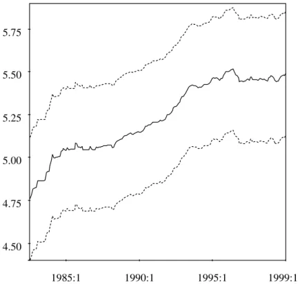
Figure 1: Fundamental value. Plot of the fundamental value of the reference house, ˆp0t, from 1982:7 to 1999:12. The series is calculated according to the fundamental value relationship given in equation (8). Confidence intervals are calculated with the delta method (see for example Greene 2000, p.357).
4.50 4.75 5.00 5.25 5.50 5.75
1985:1 1990:1 1995:1 1999:12
inverse capitalization rate θ with different relative administration costs that range from 0% up to 12.5%. According to these figures, the inverse capital- ization rate lies between 0.39% and 0.44%. If we round up to the third digit we obtain for any of these values
ˆ
ρ = 0.996. (31)
With this result at hand, we can calculate the fundamental value p0t with d0t and the relationship given in equation (11). The series from 1982:7 to 1999:12 is plotted in Figure 1. We see immediately that the value soars in the first years of the Eighties and in the first half of the Nineties. It reaches its peak in 1995. After then, the value remains on at a relatively constant level. Starting in 1985 the value resembles roughly the shape of the yearly single-family house price index of the Ring Deutscher Makler (RDM). The
RDM is an association of German realtors and valuers that conducts every year an inquiry of its members about the situation of the real estate market.
The index can be used as an rough market indicator. For the first years of the Eighties, this index shows a behavior that is different from the fundamental value. Whereas this index remains on a plateau, the fundamental value tightens during that period. However, this behavior of the fundamental value is in accordance with the RDM rent index, which was increasing during that period.
4.2 Model Selection for the Data
The size of the lot, the size of the floor space and the age of the building are the continuous variables in our model selection procedure. λ∗ chosen for our data consists of λ1 = 1 (size of the lot), λ2 = −2 (size of the floor space), andλ3 =−0.5 (age of the building). The value of the cross-validation criterion in (28) for these transformations is 0.7583. Furthermore, we obtain for our regression—where we have included an overall constant— a degree of determination of R2 = 0.7852 and an adjusted degree of ¯R2 = 0.7736.
The final model contains, in addition to the three continuous characteris- tics, sixteen characteristics. The additional characteristics are: dummies for detached house and row house (excluded category is semi-detached house), dummies for Wilmersdorf, Zehlendorf, and Steglitz (Charlottenburg is ex- cluded), dummies for houses ingood condition or inbad condition (excluded category is normal condition), a dummy fornoise in the environs of the house (e.g. the object lies in the air lane or near a railway track), a dummy for a indoor pool, a dummy for houses with valuable inventory (e.g. built-in kitchen, furniture, sauna), a dummy if the house isvacant and not occupied by the seller, a dummy for houses still under construction at the date of the sale, a dummy if the object is rented out (and thus, the buyer is an investor who wants to accrue rent payments), a dummy if the house is purchased by former tenant, a dummy if personal circumstances exist (e.g. sale between relatives or a divorced couple), and eventually a dummy if the transaction shows unusual—legal or financial—circumstances (e.g. payment by install-
ments, right of residence for the former owner).
We want shortly explain the different tax and assistant dummies that we have incorporated in the selection procedure. Before 1987, the notional rent of owner-occupied housing was taxed—just like ownership of rented objects—
through the income tax. On the other hand, it was possible to deduct de- preciation cost from the tax bill. In 1987, the taxation of the notional rent for owner-occupied housing was repealed. However, the deduction possibili- ties were modified only slightly. To catch up possible effects of this change in taxation we have generated a dummy for all owner-occupied houses that are sold before 1987. But the estimated coefficient is not significant at the 5% level. A plausible explanation is that the value of the notional rent was a (low) flat sum and that the owner had many possibilities to decrease his tax bill. So, in most cases the net effect was zero or even positive and the repealing of the tax in 1987—combined with the slight modification in the deduction possibilities—had no positive effect at all on the present value of a owner-occupied house.
In 1993, the maximal amount of purchase cost that is deductible from the income tax was halved for objects that were older than 3 years. We have captured this effect with a dummy for all objects that were sold after 1992 and were older than three years at the date of the purchase. The coefficient for this dummy is also insignificant. One possible explanation is that the overall effect is only marginal or is not identifiable because most sellers had not the right to claim for the deduction (because their income was too high or because they have already claimed the deduction in former years).
In 1996, the whole system to promote owner-occupied housing was changed.
Instead of assisting through deduction possibilities, the law Eigenheimzula- gengesetz introduced direct allowance for owner-occupied houses. However, it was the intention of that law to continue the pre-existing rules. We have generated a dummy for all owner-occupied houses that were sold after 1995.
The coefficient for the dummy is insignificant. That shows that the new law really continues the old arrangements.
Eventually, the rate of the sales tax—Grunderwerbssteuer—was increased in 1997 from 2% to 3.5%. Due to the fact that sales between direct relatives
and couples are exempted from this tax, we have generated a dummy for this change in taxation. But even for this dummy, the respective coefficient is insignificant. A possible explanation is that we have used the variable personal circumstances as indicator for sales between relatives and couples.
This variable contains also sales between companies and employees and we are unable to distangle such sales.
Furthermore, there are some other taxes that influence the net rent of a house. An example is the Grundsteuer—real estate tax—that is collected by the Federal State. However, there were no large changes of this tax and there are only few exemptions from this tax, so that we neglect it.
Perhaps, there is also a generalized explanation for the failure to identify effects of taxes and subsidies. The amount of assistance depends on the specific characteristics of the household (for example the number of kids) and not on the house per se. It is impossible to identify any effect without detailed information on sellers and buyers.
To select the financial indicators, we run a regression of the estimated coefficients of the time dummies from (27). Let ˆIt denote the estimated coefficient multiplied with minus one (recall that It≡κ−rψ,te ). Then we fit
Iˆt+1 =c+φIˆt+sTtγ+νt (32) and select the significant financial indicators. The vector of the financial indicators contains lagged values of the inflation rate for Berlin, the return of the DAX, the range of mortgage rates from different banks, and spreads between mortgage and interest rates with different interest rate fixedness and—respectively—maturities (for a study, which explores the behavior of the spreads in detail, see Nautz and Wolters 1996). For the selected model the p-value of the F-test is 0.000 and R2 = 0.7835. The estimated value of φ is 0.788 and that of σ2ν is 0.0048. The only indicators with significant coefficients at the 5% level are the spread with a fixedness of two years and the range with interest rate fixedness of five years. We have tested both series for a unit root with the augmented Dickey-Fuller test. For the test, we have included a constant and the one period lag. We can reject the hypothesis of a unit root for the spread at the 10% level. The test statistic is -2.81 and
thus very close to critical value for the 5% level, -2.87. For the range, we can reject the unit root hypothesis at the 5% level.
4.3 Results from the Estimation Procedure
We use the selected transformed variables, the two financial indicators and the estimated coefficients to initialize the EM algorithm. After each iteration, the value of the log-likelihood function in the prediction error decomposition form (23) is calculated. The results are given in Table 2. If we compare these
Table 2: Estimation output for the coefficients in the system matrices Coefficient t-Statistic Prob.
φ 0.9408 35.526 0.0000
σ2˜ν 0.0002 0.61131 0.3309 σ2ε 0.0560 45.985 0.0000
Note: convergence of the EM algorithm is reached after 5 iterations. Results are calculated with a final scoring step. The value of the log-likelihood is 1.5% higher compared with the value evaluated at the OLS estimates.
result with the OLS estimates we see immediately that the AR-coefficient of the return equation has increased substantially. On the other hand, the variance of the expected return deviations is not different from zero. It seems as if the AR-coefficient has soared much of the variance. The estimated variance of the price equation is almost unchanged. This is also true for the other coefficients of the price equation that are reported in Table 3.
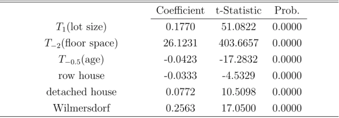
Table 3: Hedonic coefficients of the price equation Coefficient t-Statistic Prob.
T1(lot size) 0.1770 51.0822 0.0000 T−2(floor space) 26.1231 403.6657 0.0000 T−0.5(age) -0.0423 -17.2832 0.0000
row house -0.0333 -4.5329 0.0000
detached house 0.0772 10.5098 0.0000
Wilmersdorf 0.2563 17.0500 0.0000
—continued—
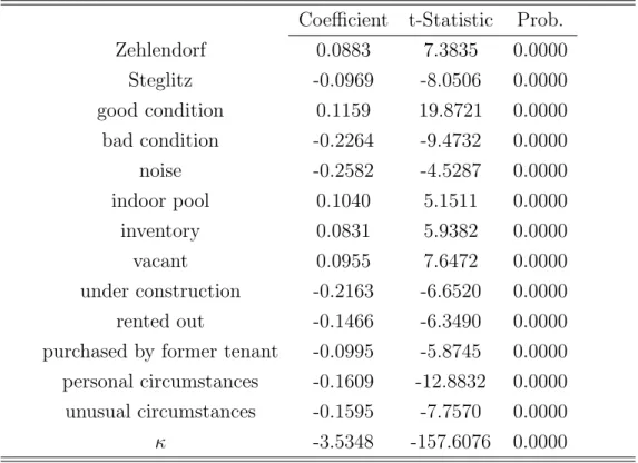
Table 3: Hedonic coefficients, continued
Coefficient t-Statistic Prob.
Zehlendorf 0.0883 7.3835 0.0000
Steglitz -0.0969 -8.0506 0.0000
good condition 0.1159 19.8721 0.0000 bad condition -0.2264 -9.4732 0.0000
noise -0.2582 -4.5287 0.0000
indoor pool 0.1040 5.1511 0.0000
inventory 0.0831 5.9382 0.0000
vacant 0.0955 7.6472 0.0000
under construction -0.2163 -6.6520 0.0000
rented out -0.1466 -6.3490 0.0000
purchased by former tenant -0.0995 -5.8745 0.0000 personal circumstances -0.1609 -12.8832 0.0000 unusual circumstances -0.1595 -7.7570 0.0000
κ -3.5348 -157.6076 0.0000
Note: estimated coefficients of the price equation (16a). The variables are explained in Subsection 4.2.
Eventually, Table 4 reports the estimated coefficients from the return equation. Compared with the results for the OLS regression of the return equation, the signs of the coefficients stay the same, but they decrease in magnitude. We will give economic interpretation for all coefficients in the next section.
Table 4: Estimated coefficients of the return equation Coefficient t-Statistic Prob.
spread2 2.0376 7.0883 0.0000 range5 -0.0238 -3.1840 0.0015
Note: estimated coefficients of the return equation (16b). spread2 is the difference between the mortgage rate with rate fixedness of two years and the interest rate with same maturity; range5 is the range of mortgage rates with interest rate fixedness of five years offered by different banks.
5 Interpretation of the Results
Starting with the hedonic coefficients ˆβ, given in Table 3, we find that the rent for a house increases both with the size of the lot and the size of the living area and decreases with the age of the dwelling. If we calculate the elasticities—evaluated at the sample mean of the respective variable—, we obtain values of about 0.29% for lot size (mean is 600 square meters), 0.6%
for floor space (mean is 170 square meters), and -0.03% for age (mean is 42 years).
Since the dependent variable is the log ratio of price and fundamental value, the coefficients of a dummy variable is approximately the percentage premium for the respective characteristic. The rent of a house with otherwise the same characteristics decreases by 3.3% if it is a row house and increases by 7.7% if it is a detached house. Here, the excluded category is a semi- detached house. As such, people are willing to pay a premium for “privacy”.
They will also pay a premium if the house lies in the districts Wilmersdorf or Zehlendorf. As we have already mentioned, there are very nice parts in these districts. Especially Grunewald in Wilmersdorf is very attractive.
The hedonic coefficient reveals that the premium is about 25%. On the other hand—compared with the reference district Charlottenburg—Steglitz charges a rebate of 9.7%.
If the house is in good condition, the rent increases by 11.6% compared with a house in normal condition. If the house is in bad condition, the rent decreases by 22.6%. The rent decreases by 25.8% if the house is located in a noisy environment in the vicinity of rail tracks, highways, or airports.
The rent increases by 10.4% if the object has an indoor pool. There is some information in the text files of our data set about the cost for construct- ing an indoor pool. The cost can go up to 100000.- Deutsche Mark. The average price for houses with indoor pool is 1.1 million Deutsche Mark, so that the hedonic coefficient is quite reasonable. If the house has inventory—
in most cases in-built kitchen and some in-built furniture—the rent increases by 8.3%. This is reasonable because such equipment is a necessary part of a house. Calculated with the average price of about 778000.- Deutsche Mark