Easy Volcanic Aerosol (EVA v1.0): an idealized forcing generator for climate simulations

(1)

www.geosci-model-dev.net/9/4049/2016/

doi:10.5194/gmd-9-4049-2016

Easy Volcanic Aerosol (EVA v1.0): an idealized forcing generator for climate simulations

Matthew Toohey^1,2, Bjorn Stevens¹, Hauke Schmidt¹, and Claudia Timmreck¹

1Max Planck Institute for Meteorology, Hamburg, Germany

2GEOMAR Helmholtz Centre for Ocean Research Kiel, Kiel, Germany Correspondence to:Matthew Toohey (mtoohey@geomar.de)

Received: 13 April 2016 – Published in Geosci. Model Dev. Discuss.: 19 May 2016 Revised: 4 October 2016 – Accepted: 17 October 2016 – Published: 11 November 2016

Abstract.Stratospheric sulfate aerosols from volcanic eruptions have a significant impact on the Earth’s climate. To include the effects of volcanic eruptions in climate model simulations, the Easy Volcanic Aerosol (EVA) forcing generator provides stratospheric aerosol optical properties as a function of time, latitude, height, and wavelength for a given input list of volcanic eruption attributes. EVA is based on a parameterized three-box model of stratospheric transport and simple scaling relationships used to derive mid-visible (550 nm) aerosol optical depth and aerosol effective radius from stratospheric sulfate mass. Precalculated look-up tables computed from Mie theory are used to produce wavelength-dependent aerosol extinction, single scattering albedo, and scattering asymmetry factor values. The structural form of EVA and the tuning of its parameters are chosen to produce best agreement with the satellite-based reconstruction of stratospheric aerosol properties following the 1991 Pinatubo eruption, and with prior millennial-timescale forcing reconstructions, including the 1815 eruption of Tambora. EVA can be used to produce volcanic forcing for climate models which is based on recent observations and physical understanding but internally self-consistent over any timescale of choice. In addition, EVA is constructed so as to allow for easy modification of different aspects of aerosol properties, in order to be used in model experiments to help advance understanding of what aspects of the volcanic aerosol are important for the climate system.

1 Introduction

Radiative forcing by variations of stratospheric sulfate aerosol from volcanic eruptions is one of the strongest drivers of natural climate variability (Crowley, 2000; Schurer et al., 2013). To reproduce the radiative forcing of past volcanic eruptions, and thereby the related climate variability, climate model simulations require estimates of the optical properties of volcanic stratospheric aerosols. Prognostic stratospheric aerosol schemes are available; however, such schemes are computationally expensive, and many of the processes underlying them are still not well understood. For these reasons, transient simulations, such as historical or millennium simulations, usually rely on prescriptive volcanic forcing reconstructions (where “forcing” hereafter refers not specifically to “radiative forcing” but rather to any external driver of climate variability prescribed in climate model simulations).

Our knowledge of past eruptions and their climate forcing is based on satellite and ground-based measurements during the recent decades, and longer-term histories can be inferred from proxies like ice cores. Different volcanic aerosol forcing sets are currently available, which use different data sources, different methodologies for combining data sources, and provide different – often incomplete – representations of aerosol properties needed for the radiative calculations of climate models.

The response of the Earth system to volcanic forcing simulated by climate models has been seen to be unrealistic in a number of prior studies. Stratospheric heating, due to the absorption of infrared radiation by volcanic aerosols, appears to be overestimated in some models (Driscoll et al., 2012).

Tropospheric cooling, while relatively realistically simulated for recent eruptions (Santer et al., 2014), appears to be too

(2)

strong in model simulations for a number of large past eruptions, most noticeably for the eruptions of Tambora in 1815 (Brohan et al., 2012) and Samalas in 1257 (Stoffel et al., 2015). Post-volcanic anomalies of atmospheric circulation, inferred from observations, are not robustly simulated by models with prescribed forcing, either at the surface (Driscoll et al., 2012), or in the stratosphere (Charlton-Perez et al., 2013). There is also a large degree of intermodel spread in the temperature response to volcanic eruptions, and even in the radiative anomalies created by prescribed volcanic forcing (Zanchettin et al., 2016). Because there are differences in the forcing data sets used, some of which may result from differences in their implementation, it remains unclear to what degree intermodel spread in response to volcanic forcing is attributable to differences in the climate models (i.e., model uncertainty) or differences in forcing (or its implementation).

In general, to isolate model uncertainty in the response to external forcings, it is desirable to have a single forcing implementation strategy, which can be applied consistently in different models. To test the sensitivity to different aspects of the forcing, and gain understanding as to what aspects of the forcing are important for the climate response, it is further desirable to have a forcing strategy which is flexi- ble enough to be used in sensitivity studies. Such motiva- tions inspired the Easy Aerosol approach to prescribed tropospheric aerosols (Voigt et al., 2014), wherein the spatial structure of tropospheric aerosols was defined by simple an- alytical functions in latitude and longitude. Building upon the Easy Aerosol approach, the MACv2-SP module provides relatively realistic representations of anthropogenic aerosol plumes with a large degree of flexibility and utility for idealized studies (Stevens et al., 2016).

We present here a description of the Easy Volcanic Aerosol (EVA) forcing generator for use in climate model simulations. EVA provides models with the full optical properties of volcanic aerosols in terms of wavelength-dependent aerosol extinction, single scattering albedo, and asymmetry factor, given an input list of eruption locations, dates, and estimated stratospheric sulfur injections. The spatiotemporal structure of the prescribed forcing aims to strike a balance between be- ing realistic (compared to modern observations) and generic, therefore producing consistent representations of eruptions over arbitrary time periods. The underlying parameterization is also readily modifiable, lending itself naturally to idealized sensitivity studies. EVA is comprised of a FORTRAN module that can be called directly by climate models, or can be used offline to produce forcing files which a model reads upon integration.

EVA builds directly upon the methods and results of pre- vious volcanic aerosol forcing reconstructions, which are briefly described in Sect. 2. The EVA approach is detailed in Sect. 3, and a brief comparison with other reconstructions is included in Sect. 4. A summary of EVA and outlook to potential uses and future versions is included in Sect. 5. A list of acronyms is provided in Appendix A.

2 Volcanic aerosol forcing: theory and practice

Volcanic eruptions impact climate primarily though the re- lease of sulfur gases, mostly in the form of sulfur dioxide (SO₂). In the atmosphere, volcanic SO₂ is chemically con- verted to sulfuric acid (H₂SO₄), which forms liquid sulfate aerosol particles (Kremser et al., 2016). Sulfate aerosols in the stratosphere tend to have typical radii of tenths of mi- crons (i.e., 0.1–1.0 µm) (Junge et al., 1961). The size distribution of stratospheric sulfate aerosol is often approximated by the log-normal distribution, described by a distribution mean and standard deviation. From a radiative standpoint, the area-weighted mean radius, or effective radius (reff), is an important property of the size distribution (Hansen and Travis, 1974).

Sulfate aerosols affect the transfer of radiation through the atmosphere. Like gases or other particulate matter, sulfate aerosols can absorb and scatter incoming radiation with a spectrally dependent signature that depends on the underlying size distribution of the aerosol. Assuming spherical aerosol particles, and based on inputs describing the size distribution and the real and imaginary indices of refraction of the material, Mie theory provides an exact solution of the radiative effects of aerosols, including the proportion of incident radiation absorbed, the proportion scattered, and the variation of scattered light with direction (Hansen and Travis, 1974). There are multiple ways of representing the resulting radiative effects; a common method (e.g., Stenchikov et al., 1998) uses the following 3 parameters: aerosol extinction (EXT) represents the total attenuation of incident radiation; the single scattering albedo (SSA) represents the proportion of EXT which is scattered (as opposed to absorbed);

and the scattering asymmetry factor (ASY) gives the average cosine of the scattering angle, weighted by the intensity of the scattered light as a function of the angle. It has a value of 1 for perfect forward scattering, 0 for isotropic scattering, and−1 for perfect backscatter. Finally, a very common parameter used to describe aerosol forcing is the aerosol optical depth (AOD), also called the aerosol optical thickness (AOT), which is the integral of the vertical profile of EXT.

The unitless AOD therefore describes the amount by which incoming radiation is attenuated through the whole atmosphere.

The gravitational settling velocity of particles of the size of stratospheric aerosol particles is small, therefore the lifetime of sulfate aerosols in the stratosphere is significant (Junge et al., 1961). Here, “lifetime” refers to thee-folding lifetime – the characteristic timescale of a chemical or physical process in which the time derivative of a quantity is proportional to its amount – defined by the time taken for a decreasing quantity to reach 1/eof its initial amount (Jacob, 1999). Given their relatively long lifetime, the transport of sulfate aerosols is largely controlled by stratospheric dynamics. The strongest winds in the stratosphere are in the zonal (east–west) direction, which act to homogenize stratospheric composition on a

(3)

fairly fast timescale (Shepherd, 2003). The Brewer–Dobson circulation (BDC) controls the distribution of stratospheric composition in the vertical–meridional plane (Holton et al., 1995; Shepherd, 2003), and is characterized by seasonally dependent two-way mixing in the midlatitudes, and a slow meridional cell of mass transport characterized by upward motion in the tropics, poleward motion in the midlatitudes, and downwelling over the poles.

The radiative effects of volcanic aerosols have been included in climate model simulations using a wide range of methods. The simplest method used involves decreasing the solar constant to reproduce the net global change in surface radiation (e.g., Metzner et al., 2014; Yoshimori et al., 2005).

This method fails to reproduce the heating of the stratosphere due to aerosol absorption of infrared radiation, and also neglects spatiotemporal variation in radiative anomalies.

On the other end of the spectrum, interactive stratospheric aerosol models explicitly simulate the evolution of stratospheric aerosols and their radiative impacts. While there is much to be learned from these models, significant uncertainties remain in the representation and coupling of aerosols, as evidenced by the large intermodel spread in standardized simulations of the 1815 Tambora eruption (Zanchettin et al., 2016). Furthermore, such models are computationally expensive, which usually prohibits their use for long-term (i.e.,

>50-year) simulations.

The most common method of including volcanic effects in climate simulations makes use of prescribed volcanic forcing data sets. Prior works have used different methods to re- construct volcanic forcing of climate, and implement these effects in climate model simulations. We briefly introduce reconstructions below which have been most often used in recent climate model simulations, and which are integral in the construction of EVA.

2.1 Sato/GISS

The Sato/GISS forcing data set (Sato et al., 1993, 2012) provides stratospheric aerosol optical depth at 550 nm (AOD₅₅₀) and aerosol effective radius (r_eff)as a function of latitude, height, and time for the period 1850–present. It is based on a mixture of satellite observations, ground-based optical measurements, and volcanological evidence. From 2001–present, the reconstruction is based exclusively on Optical Spectro- graph and InfraRed Imager System (OSIRIS) satellite measurements (Bourassa et al., 2008). For eruptions before the satellite era, the spatial structure of the AOD₅₅₀ is approximated, based on roughly scaled versions of observed eruptions, or global or hemispheric means. Aerosol effective radius is given as an empirical function of AOD₅₅₀, based on retrievals of AOD andr_efffollowing the Pinatubo eruption.

2.2 Ammann et al. (2003)

The Ammann et al. (2003) reconstruction provides AOD₅₅₀ as a function of latitude, height, and time for the period 1890–1999. It is based on estimates of the mass of SO₂injected into the stratosphere,M_SO₂, from past eruptions. The spatial structure of the AOD₅₅₀is produced by a parameterized stratospheric transport routine, representing the growth of AOD, its decay due to cross-tropopause transport, and transport from tropics to high latitudes. Compared to the Sato/GISS reconstruction, this method provides a consistent representation of volcanic forcing for all eruptions; however, it clearly simplifies the volcanic cloud evolutions compared to the observed evolutions of eruptions like Pinatubo.

2.3 Gao et al. (2008)

Building on prior work (Robock, 1981; Robock and Free, 1995), the Gao et al. (2008) reconstruction provides stratospheric sulfate aerosol mass as a function of latitude, height, and time for the period 500–2000, as well as estimates of SO₂injection by individual volcanic events over the same period. SO₂injections are based on ice core records of sulfate flux from Greenland and Antarctica. Using different scaling factors for tropical and extratropical eruptions based on nuclear bomb tests and modeling studies, ice-core-derived sulfate surface deposition rates are scaled to SO₂injections (Gao et al., 2007). Sulfate aerosol mass time series, as a function of latitude and height, were produced using a modified version of the parameterized stratospheric aerosol transport scheme of Grieser and Schönwiese (1999). Conversion of sulfate aerosol mass to radiative properties was left to the implementation of the model, but a linear scaling of aerosol mass to AOD is a commonly used assumption (Schmidt et al., 2011).

2.4 Stenchikov

The Stenchikov reconstruction provides monthly mean zonal averages of stratospheric aerosol extinction, single scattering albedo, and asymmetry factor as a function of time, pressure, and wavelength, for the period from 1850 to 1999 (Driscoll et al., 2012; Schmidt et al., 2013). This data set was used by the Max Planck Institute Earth System Model and the Geophys- ical Fluid Dynamics Laboratory’s coupled model for historical simulations as part of the Coupled Model Intercompari- son Project’s fifth phase (CMIP5). It is an extended version of the Pinatubo aerosol data set developed by Stenchikov et al. (1998) on the basis of satellite measurements of aerosol extinction and r_eff after the Pinatubo eruption. For earlier eruptions, it is based on the Sato/GISS AOD₅₅₀ andr_effre- construction. Stratospheric background aerosols are ignored, and only sulfate aerosols arising from volcanic eruptions are accounted for.

(4)

2.5 Crowley and Unterman (2013)

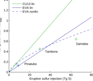
The Crowley and Unterman (2013; hereafter CU13) reconstruction, as an update to prior work (Crowley, 2000), provides AOD₅₅₀ andr_eff in four equal-area latitude bands for the time period 800–2000. It is based on ice core records of sulfate flux from Greenland to Antarctica. Ice core sulfate fluxes are scaled to peak AOD₅₅₀: for eruptions of Pinatubo magnitude and smaller, this scaling is linear and based on the ratio of satellite-observed SH AOD and the flux of sulfate to Antarctica. For stronger eruptions (like Tambora), CU13 uses nonlinear scaling first introduced by Crowley (2000), setting AOD550proportional to the two-thirds power of sulfate flux.

AOD time series were constructed based on assumptions of linear increase to peak value, a plateau, followed by exponen- tial decay with a 12-month timescale. As in the Sato/GISS reconstruction, effective radius is prescribed as a simple empirical function of AOD.

2.6 CCMI/SAGE_4λ

The aerosol forcing constructed for use in the Chemistry- Climate Model Initiative (CCMI; Eyring and Lamarque, 2013) provides aerosol optical properties EXT, SSA, and ASY as a function of wavelength, latitude, height, and time for the period 1960–present. It also provides internally consistent estimates of aerosol surface area density necessary for stratospheric chemistry simulations. The cornerstone of the CCMI forcing set is the four-wavelength SAGE II extinction data (SAGE_4λ), retrieval version 7, which span the period 1985–2005. During the SAGE II period, the four-wavelength extinction data are used to derive estimates of aerosol effective radius, from which the properties EXT(λ), SSA(λ) and ASY(λ)are derived assuming a single log-normal particle size distribution (Arfeuille et al., 2013). For other time periods, aerosol radiative properties are estimated mainly through single wavelength extinction retrievals from satellite instruments, and the observed correlation between mean aerosol radius and aerosol extinction during the SAGE II period. From 1979 to 1985, the reconstruction is based on single wavelength extinctions measured by the SAM II and SAGE I satellite instruments (Thomason and Peter, 2006).

The 1960–1979 pre-satellite period has been constructed from SAGE-II background measurements in the late 1990s, superimposing the volcanic eruptions of Agung (1963) and Fuego (1974). These eruptions were calculated by means of the AER 2-D aerosol model (Arfeuille et al., 2014; Weisen- stein et al., 1997), and the results were scaled by means of stellar and solar extinction data (Stothers, 2001). The 2006–

2011 period is derived from CALIPSO 532 nm backscatter data. An update to the CCMI reconstruction will be used in the historical simulations (1850–present) within the Coupled Model Intercomparison Project phase 6.

The observational data sets used in the CCMI reconstruction have data gaps, in particular when the atmosphere be-

came opaque directly after volcanic eruptions, which oc- curred mainly in lower tropical altitudes (below 16 km), and in the high-latitude polar regions due to limited geographical sampling of the satellite instruments (Eyring and Lamarque, 2013). After the eruptions of El Chichón and Pinatubo, data gaps were filled by means of lidar ground station data and interpolation. The remaining data gaps were filled using a linear interpolation approach in altitude and latitude.

3 The EVA approach 3.1 Basis and input data

The construction of EVA relies extensively on observational constraints. Additionally, when observations cannot adequately constrain EVA parameterizations, EVA is constructed so as to produce reasonable agreement with prior forcing sets. Data sets that were instrumental in the EVA construction include the following:

– The estimate of total SO₂ injection by Pinatubo of 18±4 Tg (9±2 Tg S) from the total ozone mapping spectrometer (TOMS) instrument (Guo et al., 2004).

– Aerosol extinction from the CCMI (Arfeuille et al., 2013). Here, we have used the CCMI data provided at http://www.pa.op.dlr.de/CCMI/CCMI_

SimulationsForcings.html, specifically the files produced for use in the ECHAM6 model. We focus primarily on the EXT at 550 nm (EXT550). AOD is computed based on the vertical integral of EXT above the climatological tropopause. Post-Pinatubo AOD and EXT anomalies are computed by subtracting an estimate of the background aerosol levels, based on the mean EXT field from the years 1999 and 2000.

– Estimates of aerosol effective radius are provided in the Sato/GISS and CU13 data sets. Approximate values of effective radius were also computed for the CCMI data set, by scaling the provided mean radius under the assumption of a log-normal distribution with an effective standard deviation of 1.2.

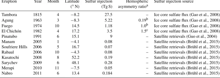
Input data, specifying the stratospheric sulfur injection properties for a number of volcanic eruptions, were collected from a range of sources and summarized in Table 1. The ice-core-derived sulfate aerosol loading estimates of Gao et al. (2008) were used to produce SO₂injection estimates for the great Tambora eruption of 1815, as well as the eruptions of Agung (1963), Fuego (1974), and El Chichón (1982). For the 1991 eruption of Pinatubo, we use the estimated total SO₂injection of 18 Tg (9 Tg S) from the TOMS instrument (Guo et al., 2004). Estimates of stratospheric SO₂injection for a number of relatively smaller eruptions in the 2000s were taken from Brühl et al. (2015), based on the MIPAS SO₂retrievals described by Höpfner et al. (2015).

(5)

Table 1.Stratospheric sulfur injection estimates used in this work.

Eruption Year Month Latitude Sulfur injection Hemispheric Sulfur injection source (^◦N) (Tg S) asymmetry ratio^a

Tambora 1815 4 −8.2 27.5 – Ice core sulfate flux (Gao et al., 2008)

Agung 1963 3 −8.3 5.22 0.19^b Ice core sulfate flux (Gao et al., 2008)

Fuego 1974 10 14.5 1.18 1.0^b Ice core sulfate flux (Gao et al., 2008)

El Chichón 1982 4 17.2 3.5 1.5^c Ice core sulfate flux (Gao et al., 2008)

Pinatubo 1991 6 15.1 9 – Satellite retrievals (Guo et al., 2004)

Manam 2005 1 −4.1 0.08 – Satellite retrievals (Brühl et al., 2015)

Soufriere Hills 2006 5 16.7 0.07 – Satellite retrievals (Brühl et al., 2015)

Rabaul 2006 10 −4.3 0.08 – Satellite retrievals (Brühl et al., 2015)

Kasatochi 2008 8 52.2 0.19 – Satellite retrievals (Brühl et al., 2015)

Sarychev 2009 6 48.1 0.28 – Satellite retrievals (Brühl et al., 2015)

Merapi 2010 11 −7.5 0.05 – Satellite retrievals (Brühl et al., 2015)

Nabro 2011 6 13.4 0.184 – Satellite retrievals (Brühl et al., 2015)

aHemispheric asymmetry ratio defined as the estimated ratio of NH/SH AOD or stratospheric aerosol loading.^bTaken as the ratio of AOD_NH/AOD_SHfor the first 2 years after each eruption from the reconstruction of Stothers (2001).^cTaken as the ratio of AOD_NH/AOD_SHfor the first 2 years after the eruption from the CCMI reconstruction (Arfeuille et al., 2013; Thomason and Peter, 2006).

3.2 Global mean AOD and effective radius

Aerosol optical depth at λ=550 nm is simulated by EVA making use of the assumption that it can be a simple function of the stratospheric sulfate mass:

AOD550=f (MSO₄). (1)

Stothers (1984) introduced a simple linear scaling between global sulfate aerosol mass and global mean AOD. Such scal- ings have a physical foundation (e.g., Charlson et al., 1992) and have long been used to study tropospheric aerosols. A linear relationship between sulfate mass and AOD has been used to convert the sulfate mass estimates of Gao et al. (2007) into radiative properties (Schmidt et al., 2011) and is implicit in the linear scaling of ice core sulfate flux to AOD used by CU13 for eruptions of Pinatubo magnitude and smaller. We apply this same assumption hereafter (up to a thresholdM∗; see Sect. 3.6) using a scaling factorA:

AOD₅₅₀=AM_SO₄, forM_SO₄< M∗. (2) Time evolution of sulfate mass is emulated in EVA using a chemical box model framework. Bluth et al. (1997) introduced a simple single-box model of stratospheric aerosol evolution. Changes in stratospheric sulfate aerosol are controlled by injections of SO2into the box, subsequent conversion of SO2into sulfate aerosols, and loss of sulfate aerosols to the troposphere. Describing the production and loss of sulfate mass (MSO₄, all masses in Tg S) as a function of the SO2

mass (M_SO₂)and characteristic timescalesτprodandτloss, respectively, the time tendency ofMSO₄ is

dM_SO₄(t )

dt =MSO₂(t ) τprod

−MSO₄(t ) τloss

. (3)

This equation describing the time evolution ofM_SO₄ can be solved analytically, for example, for a single pulse injection

ofMSO₂ at timet0: M_SO₄(t )=M_SO₂(t₀)

1−exp

−t τprod

exp

−t τloss

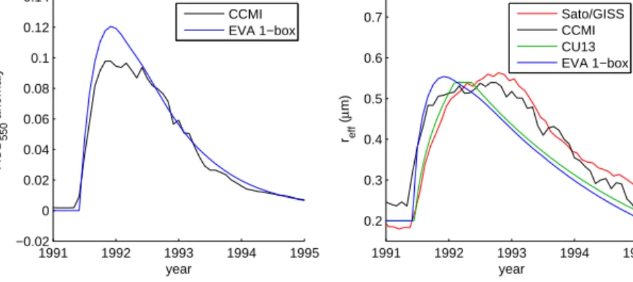
. (4) Equations (2) and (4) can be used to emulate the observed global mean AOD evolution after the Pinatubo eruption. Us- ing the best estimate of a total SO2injection of 9 Tg S (Guo et al., 2004), the parameters A,τprod, and τloss can be de- termined based on comparison with the CCMI global mean AOD anomaly time series (Fig. 1). Given the uncertainties in the CCMI AOD in the first months after the Pinatubo eruption due to the gap in the SAGE II observations due to saturation effects (Thomason and Peter, 2006), we have based our fit on the CCMI AOD beginning in July 1992, when SAGE II retrievals of the full tropical stratosphere resumed.

Therefore, the fit is not strongly constrained by the peak of global mean AOD in the CCMI reconstruction, but rather by the shape of the AOD decay. Best fit is achieved with values ofA=0.0364,τ_prod=180 days, andτ_loss=330 days.

The resultant value of A is comparable to that suggested by Stothers (1984), whose scaling factor is 0.0267 when con- verted into units of massS rather than mass sulfate aerosol, and the stratospheric loss rate (τloss=330 days) is consistent with the decay rate of AOD after Pinatubo noted by other researchers (e.g., Bluth et al., 1997). The best fit production rate,τprod=180 days, is perhaps surprising, given its discrepancy from the observed timescale of SO₂decay, which is around 30–35 days (Bluth et al., 1992; Read et al., 1993). In their single-box aerosol model, Bluth et al. (1997) noted the resulting lag between peak observed AOD and the peak in modeled SO₄ mass when using an SO₄production timescale equal to the observed SO₂decay rate, and proposed that the rate of SO₄aerosol increase may be limited by other chemical steps other than the destruction of SO₂. We contend

(6)

1991 1992 1993 1994 1995

−0.02 0 0.02 0.04 0.06 0.08 0.1 0.12 0.14

year AOD550 anomaly

CCMI EVA 1−box

1991 1992 1993 1994 1995

0.2 0.3 0.4 0.5 0.6 0.7

year reff (μm)

Sato/GISS CCMI CU13 EVA 1−box

Figure 1.Left: global mean AOD₅₅₀anomaly time series from CCMI (Arfeuille et al., 2013) following the Pinatubo eruption, and the reproduction via the EVA, single-box model approach (see text). Right: global mean aerosol effective radius time series from the reconstructions of Sato/GISS (Sato et al., 1993, 2012), the CCMI data set, CU13 (Crowley and Unterman, 2013) and the EVA single-box model approach.

that global mean AOD may further depend on the timescale of spatial spreading of the aerosol cloud, since the impact of aerosol contained within a horizontally contained vertical column will be diminished due to shielding effects. What- ever the mechanism responsible,τ_prodshould be interpreted as an effective production timescale, which incorporates not only the chemical conversion of SO₂to SO₄but other processes which damp the rise in AOD. An important caveat of this construction is that the peak loading of the simulated SO4mass is significantly less than what would result from a complete conversion of SO2to SO4prior to any loss. For this reason, the scaling factorAis larger than what would be deduced if the peak SO4loading is assumed to be equal to the SO₂injection (in Tg S). Finally, we note that since estimates of the mass of SO₂injected by Pinatubo (9±2 Tg S, from Guo et al., 2004) have an uncertainty of about 25 %, the uncertainty in the scaling factorAis at least this large.

The global mean effective radius is computed based on a simple scaling argument. For a given mass of sulfateM_SO₄, which is distributed equally amongNaerosols of radiusr,

M_SO₄∼N r³. (5)

IfN is constant, then particle radius scales as the one-third power of MSO₄. This relationship is similar to that used by CU13, who based reff on the one-third power of AOD₅₅₀. This follows if r is linearly related to reff, which is the case, for instance, if the aerosol particles are distributed log- normally by size (with a given shape parameter). In EVA, we set

r_eff=R M_SO₄¹₃

, (6)

and find a scaling constantRthat produces best agreement in terms of the peak global meanr_effreached after the Pinatubo eruption in the r_eff time series of the observation-based reconstructions. Like CU13, we also set a minimum r_eff of 0.2 µm. With a fit value ofR=0.78, the resulting EVAr_eff

time series shows reasonable agreement in peak magnitude compared to the Sato/GISS, CCMI, and CU13 reconstructions with peak values between 0.5 and 0.6 µm (Fig. 1b). Bas- ingr_effdirectly on the sulfate mass in this way does not allow the reproduction of some observed features of ther_eff evolution apparent in the Sato/GISSr_eff reconstruction, including the lag of its peak compared to that of AOD₅₅₀. How- ever, given the simplicity of this approach, and the uncertainties inreff estimates retrieved from satellite sensors, the scaling methodology appears to produce satisfactory results, and even if the Sato/GISS evolution ofreff is more realistic, it remains to be demonstrated that this difference has any detectable influence on the climate.

3.3 Spatiotemporal structure

The stratosphere can be separated into regions with dis- tinct dynamical regimes (Plumb, 1996, 2002). One important distinction is that of the relatively undisturbed tropical pipe – where mean residual motion is predominantly upward – from the extratropics, where wave breaking leads to quasi-horizontal mixing, motivating the term “surf zone”

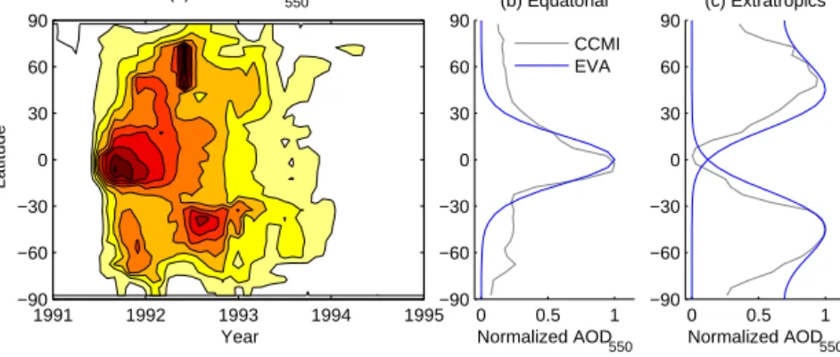
(McIntyre and Palmer, 1983). The structure of stratospheric trace-gas species are well reproduced by the so-called “leaky pipe” model of the stratosphere, which differentiates between the different dynamical regimes of the tropics vs. extratropics (Ray et al., 2010). Following these studies, and moti- vated also by the clear separation of tropical vs. extratropical stratospheric aerosol maxima following the 1991 Pinatubo eruption (Trepte et al., 1994, and Fig. 2), EVA uses a simple three-box representation of the stratosphere, separating it into three regions – equatorial, Northern Hemisphere (NH) extratropical, and Southern Hemisphere (SH) extratropical – and describes the stratospheric aerosol distribution as the su- perposition of three zonally symmetric, global-scale aerosol plumes.

The aerosol properties of each plume are defined using a static characteristic spatial structure based on extinction

(7)

(a) CCMI AOD₅₅₀

Year

Latitude

1991 1992 1993 1994 1995

−90

−60

−30 0 30 60 90

0 0.5 1

−90

−60

−30 0 30 60 90

Normalized AOD₅₅₀ (b) Equatorial

CCMI EVA

0 0.5 1

−90

−60

−30 0 30 60 90

Normalized AOD₅₅₀ (c) Extratropics

Figure 2.Definition of latitudinal shape functions.(a)The zonal mean CCMI AOD anomaly at 550 nm as a function of latitude and time for 4 years.(b)CCMI AOD anomaly averages over the 3 months (gray) after the Pinatubo eruption, normalized by its maximum value. A Gaussian fit to the equatorial portion of the 3-month average (blue) is used to define the latitudinal shape function for the equatorial plume of EVA.(c)The residual of the CCMI 4-year mean AOD minus the EVA equatorial shape function (gray) is used to define the extratropical EVA shape functions (blue).

from the CCMI reconstruction following the 1991 Pinatubo eruption. To reproduce the observed meridional structure of AOD, we choose for simplicity Gaussian functions, fit as a function of the area-conserving coordinate sin(ϕ), where ϕ denotes latitude. The observed evolution of zonal mean AOD550after Pinatubo (Fig. 2a) shows a clear separation between the three regions, with an initial growth of AOD550

within the equatorial region and later peaks in the NH and SH. We base the structure of the equatorial shape function on the CCMI AOD₅₅₀ averaged over the first 3 months after Pinatubo, before much transport to the extratropics oc- curred, and fit a Gaussian function to the central portion of the AOD₅₅₀ (Fig. 2b). (While the magnitude of AOD₅₅₀ in the first months is assumed to be highly uncertain during the first months due to saturation effects, we necessarily assume here that the latitudinal structure of the CCMI AOD is reasonably realistic.) Subtracting the Gaussian fit of the equatorial plume from the 4-year mean AOD₅₅₀isolates the spatial structure of the remaining extratropical regions (Fig. 2c). We fit the observed extratropical AOD structure with Gaussian functions centered at 45^◦with a width of 14^◦. At high latitudes, where the impact of our choice of the sin(ϕ)coordinate is strongest, the EVA fit shows some disagreement with the CCMI AOD, but much better agreement with the older Sato/GISS reconstruction (not shown). Given that SAGE observations are generally limited to ±60^◦ and high-latitude values are extrapolated, and that high-latitude aerosol often resides at heights below 15 km which can be difficult for satellite sensors to retrieve (Ridley et al., 2014), it does not appear warranted to change the sin(ϕ)fitting procedure adopted at lower latitudes.

The three horizontal shape functions are normalized by their respective global area-weighted mean. In this way, multiplication of a horizontal shape function by the sulfate mass in the region gives, for each latitude, a representation of the local vertically integrated sulfate mass density (kg km⁻²).

The time evolution of the AOD₅₅₀for each region is based on expanding the single-box model of the stratosphere of Sect. 3.2 into a three-box model. In addition to injections of SO2 and loss of sulfate through cross-tropopause transport – as in the global single-box model – sulfate is trans- ported between the three boxes, with time constantsτmixand τresdefining the rates of two-way mixing and poleward residual circulation, respectively. For example, the rate of change of sulfate mass in the NH region is related not just to SO₂- to-SO₄conversion and loss but also to mixing, which is related to the difference of mass between the NH and equatorial plumes, and the transport of mass from the equatorial plume due to the residual mass circulation of the Brewer–Dobson circulation:

dM_SO^NH

4

dt =M_SO^NH

2

τprod

−M_SO^NH

4

τloss

+

M_SO^EQ

4−M_SO^NH

4

τmix

+M_SO^EQ

4

τres

. (7) Similar expressions are used for the SH and equatorial regions. In the EVA module code, the differential equations describing the time tendency of SO4within each region are computed numerically through a forward Euler method:

M_SO₄(t+1)=M_SO₄(t )+1M_SO₄(t ) . (8)

Each eruption is treated as an instantaneous injection of SO₂ into one of the three boxes, with the injection region based on the latitude of the volcano, and latitudinal bound- aries set to±25^◦ based on satellite-based estimates of the edges of the stratospheric tropical pipe (Neu et al., 2003).

In this way, the impact of multiple eruptions occurring with overlapping time periods of impact can be easily handled, as each eruption simply adds to the pre-existing sulfur loading.

The observed AOD₅₅₀ after Pinatubo shows clear influence of the seasonal cycle of stratospheric transport, with

(8)

(a) CCMI AOD 550

Year

Latitude

1991 1992 1993 1994 1995

−90

−60

−30 0 30 60 90

AOD

0 0.05 0.1 0.15 0.2 (b) EVA AOD

550

Year

1991 1992 1993 1994 1995

−90

−60

−30 0 30 60 90

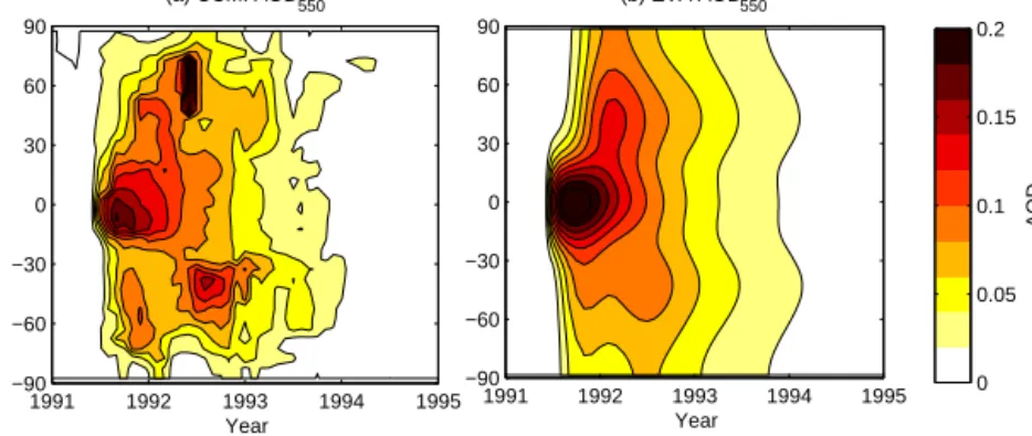
Figure 3.Aerosol optical depth (λ=550 nm) evolution after Pinatubo from (left) the CCMI database and (right) emulated by EVA.

370

370 400

400 430

430

460 460

490 490

Latitude

Altitude (km)

(a) CCMI EXT₅₅₀ (km⁻¹)

−905 −60 −30 0 30 60 90

10 15 20 25 30

0 0.5 1

−10

−5 0 5 10

(b) Equatorial

Normalized EXT 550 Δz wrt zcenter

0 0.5 1

−10

−5 0 5 10

(c) Extratropics

Normalized EXT 550 Δz wrt zcenter

Figure 4.Definition of EVA vertical shape functions.(a)CCMI aerosol extinction averaged over the first 4 years after the Pinatubo eruption, as a function of latitude and height. The climatological tropopause is shown in black and climatological July potential temperature (K) surfaces shown in gray for values as labeled. The EVA vertical center line (z_center), as defined in text, is shown in blue.(b)Normalized CCMI 4-year post-Pinatubo average extinction profiles as a function of altitude with respect to the vertical center line for the tropical (−15 to 15^◦N) latitudes (gray), and the Gaussian fit defining the EVA vertical shape function for the equatorial plume (blue). Panel(c)is the same as(b)for extratropical (30–60^◦) profiles.

maximum extratropical AOD found in the winter and spring seasons of each hemisphere, qualitatively consistent with the seasonal cycle of the Brewer–Dobson circulation which max- imizes in the winter months (Holton et al., 1995). We therefore vary theτ_mix andτ_res parameters with calendar month m, using simple sinusoidal relationships, such as

τ_mix^NH(m)=τ_mixh

1+Bcos

(m−1)π 6

i ,

m∈ {1,2, . . .,12}, (9) where the factorB describes the amplitude of the seasonal variation. Mixing and residual transport in the NH are thus strongest in January and weakest in July, and have an annual average equal toτmixandτres, respectively. Mixing and residual circulation in the SH are phase shifted by 6 months with maximum mixing in July and minimum in January. The mixing and residual transport timescales are equal for both hemispheres, and in the long term, produce relatively even partitioning of sulfate between the NH and SH. A method to reproduce hemispherically asymmetric aerosol evolution is described in Sect. 3.6.

Fitting the parameters B, τ_mix, and τ_res was achieved by minimizing the root mean square residuals of the EVA AOD₅₅₀ with the CCMI AOD₅₅₀ field for Pinatubo. Ow- ing again to the larger uncertainties in satellite-based aerosol properties in the initial months after Pinatubo due to saturation effects, the fitting procedure ignored the initial 12 months between the latitudes between 20^◦S and 20^◦N.

Best fit was achieved with values ofτ_mix=15 months,τ_res= 17 months, andB=0.75, resulting in good agreement with CCMI AOD550 evolution (Fig. 3). The AOD550 evolution of EVA lacks the fine detail of the CCMI data set, but reproduces the general spatiotemporal structure, including the double peak structure in the SH midlatitudes, and the gradual shift from strongest AOD₅₅₀in the tropics to the extratropics with time.

In the vertical dimension, observations show that volcanic aerosol extinction values were strongly peaked in the tropics at about 22 km in the first months after the Pinatubo eruption, and thereafter spread somewhat with height, with the peak shifting slightly downwards (Arfeuille et al., 2013).

(9)

Latitude

Altitude (km)

(a) CCMI EXT₅₅₀

−905 −60 −30 0 30 60 90

10 15 20 25 30

Latitude (b) EVA EXT₅₅₀

−905 −60 −30 0 30 60 90

10 15 20 25 30

Extinction (km)−1

1.5 3 4.5 6 x 107.5⁻³

Figure 5.Aerosol extinction (λ=550 nm) profiles for the 4-year post-Pinatubo average from(a)the CCMI database and(b)emulated by EVA.

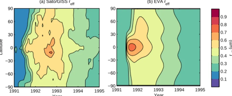
(a) Sato/GISS r_eff

Year

Latitude

1991 1992 1993 1994 1995

−90

−60

−30 0 30 60 90

(b) EVA r_eff

Year

1991 1992 1993 1994 1995

−90

−60

−30 0 30 60 90

reff (μm)

0.1 0.2 0.3 0.4 0.5 0.6 0.7 0.8 0.9

Figure 6.Zonal mean effective radius after Pinatubo from the(a)Sato/GISS reconstruction and(b)EVA.

Transport of aerosol from the equatorial region to midlatitudes and high latitudes was episodic in the first year after Pinatubo with contributions from both the lower and upper branches of the Brewer–Dobson circulation (Trepte et al., 1993). Horizontal transport of passive dynamical tracers in the midlatitude stratosphere takes place predominantly along isentropic surfaces, due to large-scale mixing processes resulting from wave activity. Aerosol transport is complicated by additional processes, including gravitational settling and anomalous vertical motions resulting from the heating of the local atmosphere by the absorption of longwave radiation by the aerosols themselves (Rogers et al., 1999). Nonetheless, the variation of peak aerosol extinction in the 4-year post- Pinatubo mean follows isentropic surfaces (derived from ERA-Interim reanalysis data; Dee et al., 2011) reasonably closely in the midlatitudes of the summer hemisphere, with the 430 K potential temperature surface corresponding well with the vertical peak of mean EXT (Fig. 4a). The correspondence between the aerosol loading and isentropic (potential temperature) surfaces breaks down in the high latitudes during winter, where diabatically driven vertical motion within the polar vortex leads to downwelling of air parcels with respect to potential temperature (Manney et al., 1994; Tegt- meier et al., 2008).

To reproduce the variation of the vertical peak of extinction with latitude in the extratropics, we define a vertical

“center line” based on climatological potential temperature.

While potential temperature does not perfectly follow the observed aerosol peak at high latitudes, by linking the vertical distribution of the aerosol to a temperature-based (rather than mass- or geopotential-based) vertical coordinate, it may be more suitable for application in much warmer or colder climates. Specifically, we define the center line at midlatitudes and high latitudes (ϕ >45^◦) from the summer 430 K potential-temperature surface for each hemisphere (July for the NH, January for the SH), and the annual mean 430 K potential-temperature surface for−45^◦< ϕ <45^◦. This em- pirically defined center line shows reasonable agreement with the observed vertical peak in aerosol extinction in the extratropics (Fig. 4a). In the tropics, the vertical position of the plume is given a vertical offset from the center line.

The vertical shape of extinction in the equatorial region is based on a Gaussian fit of the 4-year Pinatubo mean CCMI extinctions with a vertical width of 2.25 km and a vertical offset of 2.75 km (Fig. 4b). In the extratropics, a Gaussian fit is produced, centered on the defined center line with a width of 2.825 km (Fig. 4c). The vertical shape functions, defined internally on a 1 km vertical grid, are normalized by their

(10)

Latitude

CCMI AOD, 1.3 μm

1991 1992 1993 1994 1995

−90

−60

−30 0 30 60 90

EVA AOD, 1.3 μm

1991 1992 1993 1994 1995

−90

−60

−30 0 30 60 90

AOD

0 0.02 0.04 0.06 0.08 0.1

Latitude

CCMI AOD, 2 μm

1991 1992 1993 1994 1995

−90

−60

−30 0 30 60 90

EVA AOD, 2 μm

1991 1992 1993 1994 1995

−90

−60

−30 0 30 60 90

AOD

0 0.02 0.04 0.06 0.08 0.1

Latitude

CCMI AOD, 3.5 μm

1991 1992 1993 1994 1995

−90

−60

−30 0 30 60 90

AOD

0 0.02 0.04 0.06 0.08 0.1 EVA AOD, 3.5 μm

1991 1992 1993 1994 1995

−90

−60

−30 0 30 60 90

Figure 7.AOD after the Pinatubo eruption for selected wavelengths from (left) CCMI and (right) EVA.

vertical sum. Therefore, multiplication of the AOD at each latitude by the normalized vertical shape function produces a profile of aerosol extinction (per kilometer).

The resulting EVA aerosol extinction structure shows good agreement with the 4-year mean CCMI Pinatubo observations (Fig. 5). The use of Gaussian vertical and horizontal shape functions results in fairly good reproduction of the strong extinction gradient at the tropopause.

The spatiotemporal structure of aerosol effective radius is based on the simulated sulfate mass time series for each latitude (i.e., a function of the three-box model and the horizontal shape functions). Effective radius is computed for each latitude and time from Eq. 6, and assumed to be constant with height through the stratosphere. The resultingreff

field shows reasonable agreement with observation-based estimates (Fig. 6); however, it appears to produce peak values which are somewhat too large, and peak too early compared to the Sato/GISS reconstruction, as apparent also in the global mean (Fig. 1).

3.4 Wavelength-dependent optical properties

The wavelength-dependent optical properties EXT, SSA, and ASY are computable via Mie scattering theory given knowledge of the extinction at a specific wavelength, and the effective radius of an assumed log-normal size distribution. EVA utilizes look-up tables, computed from Mie theory, assuming a single-mode log-normal size distribution with width parameterσ=1.2, which gives wavelength-dependent EXT

scaling ratios (with respect to EXT at 550 nm), ASY, and SSA for varying effective radii, ranging from 0.2 to 1.3 µm, and for 29 wavelengths ranging from 0.2 to 100 µm. There- fore, given the EXT₅₅₀andreffat any point in space, EXT(λ), SSA(λ), and ASY(λ) are calculated from the lookup tables through bilinear interpolation. The use of σ =1.2 is roughly consistent with that deduced from observations of the Pinatubo aerosol cloud, with Stenchikov et al. (1998) us- ingσ=1.25 and the CCMI reconstruction usingσ=1.2 in gap-filled regions when the SAGE measurements cannot be used to estimate sigma directly (Arfeuille et al., 2013).

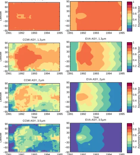
Resulting zonal mean AOD at three sample wavelengths are shown in Fig. 7 and compared to the corresponding CCMI values. In general, EVA reproduces the decrease of AOD with increasing wavelength from the visible to the near infrared. SSA and ASY at four wavelengths, at 20 km, are shown in Figs. 8 and 9, and again reproduce reasonably well the variation of magnitude with changing wavelength. Some differences in the spatial structure of SSA are apparent between the EVA and CCMI reconstructions, although it remains to be shown how important such structure is in the overall climate impact of the volcanic forcing.

3.5 Background aerosol forcing

Satellite observations of aerosol extinction in the years following the 1991 Pinatubo eruption show that the extinction approaches a non-zero minimum value. The assumption that radiative forcing by stratospheric aerosol would decay

(11)

CCMI SSA, 0.53 μm

Latitude

1991 1992 1993 1994 1995

−90

−60

−30 0 30 60 90

EVA SSA, 0.53 μm

1991 1992 1993 1994 1995

−90

−60

−30 0 30 60 90

Single scattering albedo

0.78 0.85 0.9 0.95 1

CCMI SSA, 1.3 μm

Latitude

1991 1992 1993 1994 1995

−90

−60

−30 0 30 60 90

EVA SSA, 1.3 μm

1991 1992 1993 1994 1995

−90

−60

−30 0 30 60 90

0.78 0.85 0.9 0.95 1

CCMI SSA, 2 μm

Latitude

1991 1992 1993 1994 1995

−90

−60

−30 0 30 60 90

EVA SSA, 2 μm

1991 1992 1993 1994 1995

−90

−60

−30 0 30 60 90

0.78 0.85 0.9 0.95 1

Year CCMI SSA, 3.5 μm

Latitude

1991 1992 1993 1994 1995

−90

−60

−30 0 30 60 90

Year EVA SSA, 3.5 μm

1991 1992 1993 1994 1995

−90

−60

−30 0 30 60 90

0 0.18 0.3

Figure 8.SSA after the Pinatubo eruption at 20 km for selected wavelengths from (left) CCMI and (right) EVA. Note different color scale for the lowermost panels.

to zero in the 2000–2010 decade has been shown to lead to non-negligible biases in climate model simulations (Solomon et al., 2011). The background stratospheric aerosol layer is thought to be a result of a combination of factors, including the episodic but ubiquitous influence of relatively minor volcanic eruptions with small stratospheric injections, and the slow and steady influx of aerosols and precursors from the troposphere into the stratosphere (Kremser et al., 2016).

A non-zero background stratospheric aerosol forcing is parameterized within EVA by specifying a constant SO₂ injection value, chosen to produce a best fit between the CCMI and EVA global mean AOD time series for the year 2000, where the observed global AOD reached a minimum (Fig. 10). This simple procedure results in a background SO2

injection estimate of 0.2 Tg year⁻¹. For comparison, using the coupled aerosol Solar-Climate Ozone Links chemistry climate model (SOCOL-AER) and CCMI retrievals, Sheng et al. (2015) have inferred a total net sulfur mass flux into the stratosphere of 0.19 Tg year⁻¹.

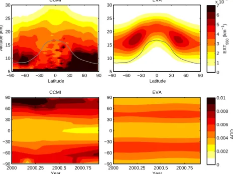
The structure of the observed aerosol extinction in the meridional height plane during the 2000 minimum is shown in Fig. 11a. Maximum aerosol extinctions in the CCMI data set are in the high-latitude lowermost stratosphere. To best reproduce this structure, the background SO₂ injections are split evenly between the two extratropical plumes.

The resulting structure of EVA background AOD forcing does not reproduce the lower stratosphere forcing due to the static shape functions of the EVA construction based on the Pinatubo aerosol evolution. Nonetheless, this strategy of background AOD in EVA does somewhat reproduce the meridional structure of the background AOD (Fig. 11c, d).

3.6 Hemispheric asymmetry

Some tropical eruptions can lead to relatively even partitioning of aerosol between the NH and SH. For example (dis- counting the likely small and short-lived impact of the Au- gust 1991 Cerro Hudson eruption), the June 1991 eruption of Pinatubo produced NH and SH AOD maxima of similar magnitude (Fig. 3). On the other hand, tropical erup-

(12)

CCMI ASY, 0.53 μm

Latitude

1991 1992 1993 1994 1995

−90

−60

−30 0 30 60 90

EVA ASY, 0.53 μm

1991 1992 1993 1994 1995

−90

−60

−30 0 30 60 90

Asymmetry factor

0.2 0.4 0.6 0.8 1

CCMI ASY, 1.3 μm

Latitude

1991 1992 1993 1994 1995

−90

−60

−30 0 30 60 90

EVA ASY, 1.3 μm

1991 1992 1993 1994 1995

−90

−60

−30 0 30 60 90

Asymmetry factor

0.2 0.4 0.6 0.8 1

Year CCMI ASY, 2 μm

Latitude

1991 1992 1993 1994 1995

−90

−60

−30 0 30 60 90

Year EVA ASY, 2 μm

1991 1992 1993 1994 1995

−90

−60

−30 0 30 60 90

Asymmetry factor

0.2 0.4 0.6 0.8 1

CCMI ASY, 3.5 μm

Latitude

1991 1992 1993 1994 1995

−90

−60

−30 0 30 60 90

Asymmetry factor

0.2 0.4 0.6 0.8 1 EVA ASY, 3.5 μm

1991 1992 1993 1994 1995

−90

−60

−30 0 30 60 90

Figure 9.ASY after the Pinatubo eruption at 20 km for selected wavelengths from (left) CCMI and (right) EVA.

19940 1995 1996 1997 1998 1999 2000 2001 2002 2003 2004 0.005

0.01 0.015 0.02

Year Global mean AOD550

CCMI EVA Sato/GISS CU13

Figure 10.Global mean AOD for the 1994–2004 period from the EVA single-box approach and the CCMI, Sato/GISS, and CU13 reconstructions.

tions like Agung (1963) and El Chichón (1982) are characterized by substantial hemispheric asymmetry in stratospheric aerosol loading. Asymmetries in the radiative forcing, if large enough, may have a detectable climate impact, for instance, through their influence on the latitude of the intertropical

convergence zone and subsequent changes in tropical mon- soon patterns (Haywood et al., 2013; Oman et al., 2006).

Some degree of hemispheric asymmetry may be expected due to the timing of an eruption with respect to the seasonal cycle of stratospheric transport. One expects tropical eruptions which occur in NH winter (when transport to the NH extratropics is strongest) to produce higher NH aerosol load- ings than those in summer. This expectation is reproduced by aerosol general circulation models (Toohey et al., 2011). The seasonal variation of stratospheric transport parameterized within EVA leads to a small degree of hemispheric asymmetry in the resulting AOD patterns depending on season of eruption, with highest asymmetry produced for tropical eruptions in August (AOD_NH/AOD_SH=1.18) and February (AODNH/AODSH=0.847).

The parameterized seasonal stratospheric transport of EVA qualitatively reproduces the observed SH bias of the AOD from the 18 February 1963 Agung eruption (Fig. 12), al- beit with much weaker magnitude. For instance, based on ground-based optical measurements, Stothers (2001) estimated that the SH aerosol loading after Agung was 8 times larger than that of the NH. Furthermore, the hemispheric

(13)

Altitude (km)

Latitude CCMI

−905 −60 −30 0 30 60 90

10 15 20 25 30

Latitude EVA

−905 −60 −30 0 30 60 90

10 15 20 25 30

EXT550 (km−1)

0 1 2 3 4 5 6 x 107 ⁻⁴

Year

Latitude

CCMI

2000 2000.25 2000.5 2000.75

−90

−60

−30 0 30 60 90

AOD550

0 0.002 0.004 0.006 0.008 0.01

Year EVA

2000 2000.25 2000.5 2000.75

−90

−60

−30 0 30 60 90

Figure 11. Top: aerosol extinction at 550 nm averaged over the year 2000 from (left) the CCMI observation-based reconstruction and (right) EVA. Bottom: AOD at 550 nm through the year 2000 from (left) CCMI and (right) EVA.

Latitude

CCMI Agung

1964 1966 1968

−90

−60

−30 0 30 60 90

EVA seasonal

1964 1966 1968

−90

−60

−30 0 30 60 90

EVA hemi. correction

1964 1966 1968

−90

−60

−30 0 30 60 90

AOD550

0 0.02 0.04 0.06 0.08 0.1

Latitude

CCMI El Chichon

Year

1982 1983 1984 1985

−90

−60

−30 0 30 60 90

EVA seasonal

Year

1982 1983 1984 1985

−90

−60

−30 0 30 60 90

AOD550

0 0.02 0.04 0.06 0.08 0.1 EVA hemi. correction

Year

1982 1983 1984 1985

−90

−60

−30 0 30 60 90

Figure 12.Illustration of hemispheric asymmetry correction in EVA. Left: CCMI representations of the zonal mean AOD for (top) Agung and (bottom) El Chichón. EVA emulations (middle) without and (right) with hemispheric asymmetry correction, as described in the text.

asymmetry produced by the seasonal stratospheric transport of EVA for El Chichón, for an 4 April eruption date, is much different than the observed strong NH asymmetry (Fig. 12).

The degree of hemispheric asymmetry for tropical eruptions may be related to the particular synoptic-scale meteorologi- cal conditions at the time and place of the initial SO₂injection, and therefore impossible to reproduce using a climatological transport parameterization.

For these reasons, an anomalous asymmetry factor is included in EVA to allow one to impose an observed asym-

metry from data. Hemispheric asymmetry can be specified in the input file, based on direct observational estimates or estimated from the ratio of Greenland to Antarctic ice core sulfate records. When this ratio differs from the asymmetry produced by the seasonal mixing parameterization of EVA, a correction can be applied which attenuates the rate of mixing and transport to one hemisphere for a period of 18 months after the eruption. This correction ensures that the AOD in the midlatitudes and high latitudes shows a hemispheric ratio