Volcanic stratospheric sulfur injections and aerosol optical depth from 500 BCE to 1900 CE

(1)

https://doi.org/10.5194/essd-9-809-2017

Volcanic stratospheric sulfur injections and aerosol optical depth from 500 BCE to 1900 CE

Matthew Toohey¹and Michael Sigl^2,3

1GEOMAR Helmholtz Centre for Ocean Research Kiel, Germany

2Laboratory of Environmental Chemistry, Paul Scherrer Institute, 5232 Villigen, Switzerland

3Oeschger Centre for Climate Change Research, 3012 Bern, Switzerland Correspondence to:Matthew Toohey (mtoohey@geomar.de)

Received: 24 April 2017 – Discussion started: 19 June 2017

Revised: 11 September 2017 – Accepted: 18 September 2017 – Published: 6 November 2017

Abstract. The injection of sulfur into the stratosphere by explosive volcanic eruptions is the cause of significant climate variability. Based on sulfate records from a suite of ice cores from Greenland and Antarctica, the eVolv2k database includes estimates of the magnitudes and approximate source latitudes of major volcanic stratospheric sulfur injection (VSSI) events from 500 BCE to 1900 CE, constituting an update of prior reconstructions and an extension of the record by 1000 years. The database incorporates improvements to the ice core records (in terms of synchronisation and dating) and refinements to the methods used to estimate VSSI from ice core records, and it includes first estimates of the random uncertainties in VSSI values. VSSI estimates for many of the largest eruptions, including Samalas (1257), Tambora (1815), and Laki (1783), are within 10 % of prior estimates.

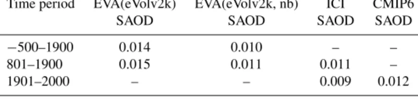
A number of strong events are included in eVolv2k which are largely underestimated or not included in earlier VSSI reconstructions, including events in 540, 574, 682, and 1108 CE. The long-term annual mean VSSI from major volcanic eruptions is estimated to be ∼0.5 Tg[S]yr⁻¹,∼50 % greater than a prior reconstruction due to the identification of more events and an increase in the magnitude of many intermediate events. A long-term latitudinally and monthly resolved stratospheric aerosol optical depth (SAOD) time series is reconstructed from the eVolv2k VSSI estimates, and the resulting global mean SAOD is found to be similar (within 33 %) to a prior reconstruction for most of the largest eruptions. The long-term (500 BCE–1900 CE) average global mean SAOD estimated from the eVolv2k VSSI estimates including a constant “background” injection of stratospheric sulfur is

∼0.014, 30 % greater than a prior reconstruction. These new long-term reconstructions of past VSSI and SAOD variability give context to recent volcanic forcing, suggesting that the 20th century was a period of somewhat weaker than average volcanic forcing, with current best estimates of 20th century mean VSSI and SAOD values being 25 and 14 % less, respectively, than the mean of the 500 BCE to 1900 CE period. The reconstructed VSSI and SAOD data are available at https://doi.org/10.1594/WDCC/eVolv2k_v2.

1 Introduction

The injection of sulfur into the stratosphere by explosive volcanic eruptions has important ramifications for the Earth’s climate. Sulfur-containing gases emitted by volcanic eruptions, including SO₂and H₂S, lead to the formation of liq- uid sulfate aerosols. In the stratosphere, sulfate aerosols have a lifetime on the order of years. These aerosols scatter in- coming solar radiation and absorb infrared radiation, leading

to a net decrease in radiation reaching the Earth’s surface and associated cooling (Robock, 2000).

Reconstructions of the history of climatic forcing by past eruptions have a long history (Lamb, 1970) and are an important ingredient in an understanding of past climate variability. Volcanic reconstructions have been extensively used to understand climate variability in instrumental and proxy- based climate records (Crowley et al., 2008; Hegerl et al., 2007; Masson-Delmotte et al., 2013; Sigl et al., 2015) and

(2)

have been used to show that volcanism is the dominant natural driver of climate variability in the Earth’s recent past (Schurer et al., 2013). Volcanic reconstructions are also in- creasingly being used to understand the role of sudden climate changes in the evolution of past societies as recorded in documentary and archaeological archives (Ludlow et al., 2013; Oppenheimer, 2011; Toohey et al., 2016a).

Volcanic forcing reconstructions provide essential bound- ary conditions for climate model simulations which aim to reproduce past climate variability. In one commonly used methodology, climate models take as input reconstructed volcanic forcing datasets, which prescribe certain physical as- pects of the volcanic stratospheric sulfate aerosol. More recently, climate models have been coupled with prognostic aerosol microphysical modules, which allow for the explicit simulation of the growth, transport, and removal of stratospheric aerosols (e.g. English et al., 2013; Mills et al., 2016;

Timmreck, 2012; Toohey et al., 2011). For these models, simulating the effects of volcanic eruptions on climate re- quires estimates of the amount of sulfur injected into the stratosphere and the time and location of that injection. Prog- nostic aerosol modelling, however, comes with an associated computational expense, and many model simulations con- tinue to use prescribed aerosol forcing sets as input. The Easy Volcanic Aerosol (EVA) forcing generator is a simple and flexible module which produces stratospheric aerosol properties for use in climate models when given the sulfur injection magnitude, time, and approximate location (Toohey et al., 2016b). EVA therefore provides the bridge necessary to allow different types of models to use time series of volcanic stratospheric sulfur injection (VSSI) as a common basis for volcanic forcing.

For eruptions since approximately 1979, VSSIs can be estimated based on satellite observations of the initial SO₂ plume (Bluth et al., 1997; Carn et al., 2016; Clerbaux et al., 2008; Guo et al., 2004; Höpfner et al., 2015; Read et al., 1993). Prior to the satellite era, information on the sulfur injection can be inferred from different records, including optical measurements (Sato et al., 1993; Stothers, 1996, 2001), geologic information on the on the eruptive magnitude and volatile content of the erupted magma (Metzner et al., 2012;

Scaillet et al., 2003; Self, 2004; Self and King, 1996), and ice cores (Ammann et al., 2003; Clausen and Hammer, 1988;

Robock and Free, 1995; Zielinski, 1995). Ice cores in particular provide long records with unequalled temporal accuracy and precision of volcanic eruptions from around the globe (Cole-Dai, 2010; Robock and Free, 1995).

Ice cores were first used to estimate the stratospheric sulfate aerosol mass burden following explosive volcanic eruptions by Clausen and Hammer (1988). Zielinski (1995) used similar techniques to estimate the sulfate aerosol loading resulting from eruptions spanning 2100 years based on chemical analysis of the Greenland GISP2 ice core. Robock and Free (1995) constructed an index of volcanic climate forcing from a compilation of multiple polar ice cores from both

hemispheres. Based on a larger compilation of ice cores, Gao et al. (2008) reconstructed both stratospheric sulfur injections and reconstructions of the spatio-temporal spread of aerosol mass in the stratosphere over the time period 501–

2000. Other volcanic reconstructions (e.g. Ammann et al., 2003; Crowley and Unterman, 2013) have provided estimates of the radiative impacts of past eruptions based on analysis of ice cores without explicitly estimating sulfate aerosol masses or sulfur injections.

Recent improvements to the ice core record of past volcanism (Plummer et al., 2012; Sigl et al., 2014, 2015) moti- vate a revision and extension of sulfur injection reconstructions. The record of volcanism preserved in Antarctic ice has been improved based on the compilation of a larger set of ice cores, extending back to 500 BCE, with a largely static number of cores used to compile an Antarctic average for the past 2000 years (Sigl et al., 2014). An adjustment to previous age models used to date past volcanic events has resulted in better agreement between ice core sulfate signals and cooling signals preserved in tree rings, improving confidence in the accuracy of the new ice core record dating (Sigl et al., 2015).

This paper describes the construction of a new sulfur injection database from ice core records based on newly compiled ice core sulfate composites. It presents the justifica- tion for a modification to the method used to convert ice core sulfate fluxes to VSSI compared to past works. Finally, we present estimates of stratospheric aerosol optical depth (SAOD) translated from the VSSI estimates presented here using the EVA forcing generator and compare the resulting record with prior reconstructions. Together, the resulting VSSI and SAOD datasets represent significant updates and improvements to the volcanic forcing datasets (Crowley and Unterman, 2013; Gao et al., 2008) used in numerous prior climate model simulations, including those used in the Pale- oclimate Modelling Intercomparison Project (PMIP) Phases 2 and 3 (Schmidt et al., 2011).

2 Method 2.1 Ice core data

Sulfate (or sulfur) in ice cores can have several sources, of which marine biogenic emissions of dimethyl sulfide and volcanic sulfur emissions are the most important contribu- tions during the pre-industrial era (Cole-Dai, 2010). All reconstructions of volcanic sulfate mass deposition from ice cores agree in the general methodology, in which the non- volcanic (or background) contribution to the total sulfate (or sulfur) at the ice core site is assumed to be slowly varying and thus can be well approximated by simple functions such as splines, running medians, or a constant value. Upon sub- tracting the estimated background from the total concentrations, the remaining excess concentrations are attributed to volcanic origin (Gao et al., 2006, 2008; Sigl et al., 2014;

Traufetter et al., 2004; Zielinski, 1995).

(3)

2.1.1 Ice core sulfate composites

As the basis of the volcanic reconstruction, we used an ex- isting compilation of synchronised volcanic sulfate records from ice cores in Greenland and Antarctica (Sigl et al., 2015) complemented with the GISP2 ice core record from Green- land (Zielinski, 1996) to improve the sampling density, especially during the earlier period of our reconstruction. The compilations use only sulfur and sulfate (SO²⁻₄ ) concentration measurements and exclude measurements of electrical conductivity or acidity since other species than sulfur (e.g.

chlorine, fluorine, nitrate, carboxylic acids) may also con- tribute to the total measured acidity (Clausen et al., 1997;

Pasteris et al., 2014). A list of ice cores used is included in Table S1. In summary, the reconstruction is based on ice cores from three sites in Greenland, including NEEM (Sigl et al., 2014, 2015), NGRIP (Plummer et al., 2012), and GISP2 (Zielinski, 1995, 1996) and between 8 and 17 individual ice cores from Antarctica included in the AVS-2k composite over the Common Era (Sigl et al., 2014) extended to earlier dates by the WDC (from 394 BCE) and B40 (from 500 BCE) ice cores (Sigl et al., 2015).

Volcanic sulfate flux is non-uniform over Greenland and Antarctica, and the shortest ice core records (in time) usually have the largest deposition rates (Gao et al., 2007; Sigl et al., 2014). Taking account of changes in the sample size and pattern over time is a challenging issue in the construction of long-term ice sheet average fluxes. To simplify this process and improve the long-term stability of the resulting records, we preferentially used the longest ice core records currently available, resulting in a relatively constant sample size over most of the Common Era (N≥12; 200–1900 CE).

With the addition of GISP2, only one ice core record has been included into the composite which was not part of the Sigl et al. (2015) database but which has been used in previous compilations (Crowley and Unterman, 2013; Gao et al., 2008). Synchronisation to the NS1-2011 chronology was performed against the NEEM sulfur record, and 85 common stratigraphic age markers (averaging one every 30 years) have been identified (Figs. S1–S3). Over the past 2500 years, the GISP2 sulfate record contains some missing data sections encompassing in total 160 years (6 %), including the time period 532–606 AD, which includes some of the largest volcanic eruptions in historic times.

Our estimates of the timing of volcanic sulfate enrich- ment in the ice cores are based on the most recently updated ice core chronologies for Greenland and Antarctica (NS1- 2011 and WD2014, respectively; see Sigl et al., 2015, 2016) and represent the first year in which a sulfate anomaly was detected in the glacio-chemical records. Small adjustments were made in cases in which bipolar eruptions had slightly different ages in Greenland and Antarctica to derive a unified chronology (Sigl et al., 2015). Since the Greenland ice core chronology (NS1-2011) was constrained with more absolute age markers than that from Antarctica (WD2014), a stronger

weight was usually given to the Greenland ages. For known historic eruptions – some of which are verified by identify- ing and characterising tephra in ice cores (Abbott and Davies, 2012; Jensen et al., 2014; Sun et al., 2014) – the exact timing (calendar date, month, season) of the eruptions was used. For the majority of the volcanic events over the past 2500 years, the exact timing of the eruption cannot be constrained with the ice core records alone, since volcanic sulfate has different atmospheric residence times depending on such details as the latitude, season, and injection height of the eruption. Thus the time lag between stratospheric injection at the source and deposition at the ice core site can vary between a few weeks up to a year (Robock, 2000; Toohey et al., 2013).

For each ice core used, deposited SO4 mass (or “flux”, in units kg km⁻²) was previously estimated for all volcanic events exceeding a predefined detection threshold by inte- grating the sulfate flux exceeding the natural background over the time span of its deposition (Plummer et al., 2012;

Sigl et al., 2013, 2014, 2015; Zielinski, 1995, 1996). While major volcanic signals related to eruptions such as Samalas (1257), Tambora (1815), Huyanaputina (1600), or Krakatau (1883) are clearly identified in all ice cores taken from a larger network, the smaller volcanic events may in some cases not be picked up by all ice cores equally. For example, analysis of the GISP2 ice core, which was measured at biannual resolution (Zielinski, 1995), detected fewer volcanic events than in comparably long but higher-resolved ice cores from NEEM and NGRIP. Low annual snowfall rates present in some areas in Antarctica can also occasionally lead to post-depositional changes in the original volcanic sulfate signature, as was shown in the example of the Tambora 1815 event using five ice cores from Dome C (Gautier et al., 2016).

Even under such extreme climate conditions present at some areas of East Antarctica, the loss of volcanic signatures from individual ice core records by wind erosion is rather the ex- ception than the rule given that the major volcanic signatures of even much smaller events are continuously captured in vir- tually all ice cores over Antarctica (Sigl et al., 2014). The large number of ice cores included in the AVS-2k network not only allowed for the firm detection of false positives and more precise quantification of total sulfate flux, but also for a reduction of the detection limit and the identification of additional events that would not exceed the threshold limits set for a single sulfate record. By using an alternative detection approach (AVS-2ks) based on extracting the event flux directly from a stacked sulfate concentration record characterised by increased signal-to-noise ratios compared to the more noisy individual ice core records, Sigl et al. (2014) extracted an additional 46 volcanic events with sulfate fluxes as low as 1–4 kg km⁻², whereas the detection limits for the individual ice core sulfate series were close to 3–5 kg km⁻². With no comparable large network available from Greenland, the detection limit for the three Greenland ice cores in pre- industrial times is typically in the range of 3–6 kg km⁻². Af- ter approximately 1900 AD, the increased anthropogenic re-

(4)

lease of SO2into the troposphere from industrial processes masks many of the volcanic signatures during the 20th century in Greenland (Fig. S3). For this reason, we have constrained the present reconstruction to the period before 1900.

For the period thereafter, we recommend the use of estimates utilising larger networks of Greenland ice cores (Crowley and Unterman, 2013; Gao et al., 2008) or from other multi- proxy reconstructions (Neely and Schmidt, 2016).

Antarctic and Greenland ice sheet average flux values were then computed based on the available ice core measurements for each volcanic event. In the AVS-2k compilation, individual ice cores were weighted in the overall average in order to account for the spatial variability of deposition over the ice sheet. This was accomplished by first averaging flux values for pre-defined regions or depositional regimes and then averaging the values over the different regions (Sigl et al., 2014). For Greenland, a simple average of the three ice cores was used, since the ice cores show no evidence of systematic differences in their measured values for 48 volcanic events common to all three cores (Fig. S4). In cases when volcanic sulfate was not detected in all three Greenland cores, sulfate flux was set to 50 % of the detection limit for those ice cores without a strong signal. This is motivated by the fact that visual inspection of the data for such cases often re- vealed the presence of a volcanic signal which did not exceed the detection threshold. These cases only include comparably small volcanic signals: the largest 40 events recorded in the Greenland ice cores since 200 CE all have signals in all three ice cores (providing no gaps in the records). Appar- ently, the detection threshold had been set differently for the individual ice cores so that many volcanic events detected in NEEM and/or NGRIP have not been extracted for the GISP2 record. NEEM also seems to extract slightly fewer events than NGRIP, potentially owing to the greater background variability of sulfur due to the closer proximity of the ice core site to the ocean emitting biogenic sulfur species.

Situated in the centre of Greenland, the NGRIP record has arguably the best ability to capture the atmospheric excess sulfate content from volcanic eruptions, and we thus argue that the simple arithmetic mean is the most realistic metric to describe the true sulfate deposition over Greenland. For Antarctica, occasionally missing values in individual cores have also not been set to “zero” prior to averaging, but the influence on the overall composite value is minimal, as is ev- ident by the comparison with the alternatively stacked composite AVS-2ks(Sigl et al., 2014).

2.1.2 Ice core uncertainties

Uncertainty in the timing of volcanic events in ice core records arises from uncertainties in the annual-layer interpretation when establishing the layer counted chronologies.

Absolute age uncertainties in the ice core records used in eVolv2k are believed to be on average better than ±2 years during the past 1500 years and better than ±5 years some

2500 years ago based on comparison to well-dated tree ring records (Adolphi and Muscheler, 2016; Sigl et al., 2015, 2016).

Since the composites for Greenland (in general) and Antarctica (prior to the Common Era) are based on a few ice cores only, we explore in the following how well large-scale sulfate flux over Greenland and Antarctica is reproduced in individual records or pairs of ice core records. For this we use 48 events that are common to all three ice core records in Greenland and 48 events that are recorded in at least 10 ice core records from Antarctica. In both cases, this threshold is more or less equivalent to eruptions with more than 6–7 kg km⁻²of average sulfate flux (Fig. S4).

For Antarctica, individual ice core records such as B40 (R²=0.88) and WDC (R²=0.91) are strongly correlated with the ice-sheet-wide flux values based on a large number (N≥10) of individual ice cores (Fig. S4). A composite of only the B40 and WDC records – which is the sample used here prior to the Common Era in Antarctica – produces quite reasonable agreement with the full Antarctic composite for the 48 common events, with a correlation ofR²=0.93.

Similarly, for Greenland, a composite of NEEM and GISP2 shows close correlation (R²=0.98) with the three-ice-core Greenland composite, and correlations of single ice core values vs. the full composite are only slightly smaller, with GISP2 (R²=0.76) showing the weakest agreement with the overall composite and NGRIP (R²=0.89) having the high- est correlation. The high level of correlation – especially over Antarctica where a large number of individual records con- tributes to the composite – indicates that the lack of repli- cation of the Tambora signal observed at Dome C (Gautier et al., 2016) is most likely a phenomenon specific to the wind-exposed Antarctic plateau and that, in general, individual ice core records are able to capture a large portion of the large-scale sulfate flux. In other words, the strong correlations between ice sheet composites and the single-site records support the idea that valuable information on large- scale sulfate flux and therefore stratospheric aerosol burdens can be extracted even from a small number of ice cores from well-placed sites.

Uncertainties in the Antarctic composite sulfate fluxes in AVS-2k are taken as reported by Sigl et al. (2015). From 1–

2000 CE, the uncertainty in the Antarctic mean is quantified by the standard error of the mean (SEM) of the individual ice core flux values. Typical (root mean square) uncertainties for this period in the Antarctic composites are approximately 13 %. Before 1 CE, when only two ice cores are used in the construction of the Antarctic composite, a constant uncertainty value of 26 % is assumed based on regression analysis between AVS-2k (the ice sheet average) and the composite of WDC and B40 over the 1–2000 CE period (see Sigl et al., 2015).

Special consideration is paid to uncertainties in the Green- land composite sulfate flux due to the small sample size. As- suming that the fluxes retrieved from each ice core represent

(5)

the true ice sheet average plus some normally distributed independent random error, estimates of the error variance for each ice core can be estimated (Appendix A). This analysis produces estimates of 46, 45, and 33 % for NEEM, NGRIP, and GISP2, respectively (Fig. S5). Using standard error propagation rules, we estimate that when all three ice cores are used in an ice sheet composite, the resulting uncertainty is approximately 22 % and two-core composites take uncertainties of approximately 32 % (NEEM plus NGRIP), 28 % (NEEM plus GISP2), and 28 % (NGRIP plus GISP2).

2.2 Injection locations and dates

The locations and dates of stratospheric sulfur injections can be assigned based on matching ice core sulfate signals with observed historic eruptions. Here, following prior work (e.g.

Crowley and Unterman, 2013; Plummer et al., 2012; Sigl et al., 2013), we use the Volcanoes of the World online eruption database (Global Volcanism Program, 2013) and other sources of information to assign locations and dates to a number of events in the combined Greenland and Antarctic sulfate event inventory (Table 1). Such matches carry some degree of uncertainty and subjectivity. In some cases, the matches can be made with a high degree of confidence based on the temporal coincidence of exceptional sulfate signals with similarly exceptional eruptions, e.g. Tambora (1815) and Laki (1783). Chemical analysis of tephra extracted from ice cores has been used to strengthen the matches for cases like Samalas (1257, Lavigne et al., 2013) and Changbaishan (946, Sun et al., 2014). In other cases, matches are based on little more than temporal coincidence between an ice core sulfate signal and an identified major eruption – such matches are prone to reexamination when ice core timescales are adjusted or the eruption catalogue is updated. For this exercise, we have attempted to err on the side of caution and have discarded some matches used in prior work. For example, the large mid-15th century ice core sulfate signal originally attributed to 1452/53 (Gao et al., 2006) and recently refined by independent annual-layer counting to 1458 (Plummer et al., 2012; Sigl et al., 2013) often attributed to the Kuwae caldera, Vanuatu (17^◦S) is considered unidentified here.

For the remaining majority of ice core sulfate signals which are not easily matched to a known eruption, approximate eruption latitudes are assigned based on the presence or lack of simultaneous signals in both Greenland and Antarc- tic ice core composites. Signals occurring synchronously (given small possible dating uncertainties) in both Green- land and Antarctic composites are attributed to tropical eruptions, while those with signals in only one hemisphere are assumed to be extratropical in origin following Sigl et al.

(2015). Representative latitudes for unidentified eruptions can be based on the latitudinal distribution of identified eruptions. Based on the Holocene eruption database (Global Vol- canism Program, 2013), we find average latitudes of extrat-

ropical (|ϕ|>25), VEI≥5 eruptions of 48^◦N and 42^◦S, and an average tropical eruption latitude of 2^◦N. For simplicity and symmetry, we adopt a convention of assigning unknown tropical eruptions a latitude of 0^◦N and extratropical eruptions a latitude of 45^◦N or S. Consistent with Crowley and Unterman (2013), unknown eruptions are assigned an eruption date of 1 January.

2.3 Stratospheric sulfate injection estimation

The mass of sulfur injected into the stratosphere by an eruption (M_S) is eventually deposited onto the Earth’s surface.

Assuming all injected sulfur is converted to sulfate aerosols before deposition, the mass of total sulfate flux to the surface (D_SO₄) is simply 3M_S due to the ratio of the molecular mass of SO4to the atomic mass of sulfur. From ice cores, the sulfate “flux” (fSO₄) is derived, which represents the local accumulated sulfate mass density in units of kg km⁻². If this flux was uniform over the Earth, estimatingDSO₄ (and therebyMS) would simply require multiplying the flux by the surface area of the Earth. Since the deposition is not spa- tially uniform, a transfer function is required to convert flux values from any location or area to estimates ofD_SO₄ to account for the spatial inhomogeneity of deposition (Gao et al., 2007; Toohey et al., 2013). Assuming that the deposition pattern is consistent for all events for any location or region on Earth, a transfer function,L^global, can be defined as

L^global=D_SO₄

f_SO₄ =3M_S

f_SO₄ . (1)

Clausen and Hammer (1988) derived the first global transfer functions based on analysis of the radioactive products of nuclear weapons testing (NWT) in the 1950s and 1960s, with L^global defined by the ratio of the estimated release of radioactive material and estimates of the radioactive flux from analysis of ice cores. Clausen and Hammer (1988) then used the global transfer functions to estimate the sulfate aerosol loading from a number of past eruptions by applying the transfer function for each ice core individually to the volcanic fluxes for each core and averaging the result for a best estimate.

Gao et al. (2007) suggested that the sulfate fluxes to Green- land and Antarctica can be used separately as proxies for the Northern Hemisphere (NH) and Southern Hemisphere (SH) sulfate loading. In this methodology, transfer functions are required to connect the ice sheet sulfate fluxes from Green- land and Antarctica (f^G,f^A, respectively, with the subscript

“SO₄” discarded hereafter for brevity) to the total hemispheric deposited sulfate (D^NHandD^SH). By defining a vari- able,α, which represents the ratio of NH to global deposited sulfate and therefore the proportion of the total sulfur injection,M_S, which is transported to and deposited over the NH, α= D^NH

D^global =1− D^SH

D^global, (2)

(6)

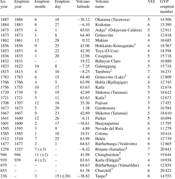
Table 1.Proposed matches of ice core sulfate signals to volcanic eruptions. Matches are based on those listed by Sigl et al. (2013), with appropriate time shift applied due to updated ice core timescales (Sigl et al., 2015), except where noted. Volcano names, eruption dates, and eruption numbers are taken from the Volcanoes of the World database provided online by the Global Volcanism Program (2013), except where noted.

Ice Eruption Eruption Eruption Volcano Volcano VEI GVP

year year month day latitude name eruption

number

1887 1886 6 10 −38.12 Okataina (Tarawera) 5 14 506

1884 1883 8 27 −6.10 Krakatau 6 15 589

1875 1875 4 1 65.03 Askja¹(Öskjuvatn Caldera) 5 12 911

1873 1873 1 8 64.40 Grímsvötn 4 12 818

1862 1861 12 28 0.32 Makian 4 16 685

1856 1856 9 25 42.06 Hokkaido-Komagatake¹ 4 18 567

1853 1853 4 22 42.50 Toya (O-Usu) 4 18 598

1836 1835 1 20 12.98 Cosigüina 5 15 718

1832 1831 – – 19.52 Babuyan Claro 4 16 880

1823 1822 10 8 −7.25 Galunggung 5 15 718

1815 1815 4 10 −8.25 Tambora² 7 16 231

1783 1783 6 15 64.40 Grímsvötn (Laki)³ 4 12 809

1766 1766 4 5 63.98 Hekla (Bjallagigar) 4 12 745

1756 1755 10 17 63.63 Katla 5 12 674

1739 1739 8 19 42.69 Shikotsu (Tarumai) 5 18 612

1721 1721 5 11 63.63 Katla¹ 5 12 673

1708 1707 12 16 35.36 Fujisan 5 17 452

1673 1673 5 20 1.38 Gamkonora 5 16 584

1667 1667 9 23 42.69 Shikotsu (Tarumai) 5 18 610

1641 1640 12 26 6.11 Parker 5 16 694

1601 1600 2 17 −16.61 Huaynaputina 6 11 795

1595 1595 3 9 4.89 Nevado del Ruiz 4 11 279

1585 1585 1 10 19.51 Colima 4 10 414

1512 1510 7 25 63.98 Hekla 4 12 739

1477 1477 2 1 64.63 Bárðarbunga (Veidivötn) 6 12 865

1258 1257 7 (±3) – −8.42 Rinjani (Samalas)⁴ 7 20 843

946 946 11 (±2) – 41.98 Changbaishan⁵ 7 19 644

939 939 4 (±2) – 63.63 Katla (Eldgjá)⁶ 4 19 938

879 – – – 64.63 Bárðarbunga (Vatnaöldur) 4 12 854

853 – – – 61.38 Churchill⁷ 6 20 422

236 – 3 15 (±20) −38.82 Taupo⁸ 6 14 553

1Newly proposed match.

2Date of most explosive phase of eruption, from Sigurdsson and Carey (1989).

3Date of most explosive phase of eruption, from Thordarson and Self (2003).

4Attribution and date estimate from Lavigne et al. (2013).

5Attribution from Sun et al. (2014). Date based on inference from historical documents (Hayakawa and Koyama, 1998; Xu et al., 2013).

6Date (including estimate of season) from Oppenheimer et al. (2017).

7Attribution from Jensen et al. (2014).

8Eruption season derived from dendrochronological evidence (Hogg et al., 2012).

we can write transfer functions for the ice sheets of each hemisphere:

L^G=D^NH

f^G =3αMS

f^G , (3)

L^A=D^SH

f^A =3(1−α)MS

f^A . (4)

From Eqs. (3) and (4), we can write an expression forM_S as a function of the measured Greenland and Antarctic fluxes and the transfer functions:

MS=L^Gf^G

3 +L^Af^A

3 . (5)

While the hemispheric partitioning coefficient α is not required to calculateM_S via Eq. (5), it can be used as a proxy for the hemispheric asymmetry of the volcanic radiative forcing. In practice, the eVolv2k database includes the ratio (R)

(7)

of the estimated NH to SH deposited sulfate:

R=L^Gf^G

L^Lf^L, (6)

whereRis simply related toαasR=α/(α−1).

Gao et al. (2007) derived values of the hemispheric transfer functions L^G andL^A separately for tropical and extratropical eruptions. For tropical eruptions, Gao et al. (2007) used measurements of nuclear radioactivity from ice cores (Clausen and Hammer, 1988) and revised estimates of the stratospheric injection of radioactive fallout from NWT.

Since the partitioning of radioactive material between the NH and SH after the NWT in the tropics is uncertain, Gao et al. (2007) assumed that between 1/2 to 2/3 of the radioactive material was transported into the Northern Hemisphere (i.e. 0.5< α <0.66), which lead to estimates forL^G rang- ing from 0.75 to 1.0×10⁹km². ForLÂ, Gao et al. (2007) used estimates of the sulfur injection by the 1991 eruption of Pinatubo and measured sulfate in Antarctic ice cores. We re- visit that calculation here based on updated data. According to analysis of satellite retrievals (Guo et al., 2004), Pinatubo injected 18±4 Tg of SO₂into the lower tropical stratosphere, amounting to 9±2 Tg [S]. Satellite records also show a fairly even transport of aerosol between the NH and SH, suggesting α≈0.5. The Antarctic average sulfate flux following Pinatubo is approximately 11 kg km⁻²(Crowley and Unter- man, 2013; Sigl et al., 2014). Using these values in Eq. (4) leads to an estimate ofLÂof 1.2±0.3×10⁹km²or approximately 0.9–1.5×10⁹km². This calculation is only slightly changed when considering the potential impact of the Au- gust 1991 Cerro Hudson eruption in Chile, which injected an estimated 0.75 Tg [S] into the stratosphere (Bluth et al., 1997). In this case, again noting that the observed SAOD after Pinatubo was balanced between the NH and SH, we infer that the SH loading was about half of the total sulfur injection by Pinatubo and Cerro Hudson, around 4.9±1 Tg[S], which leads to a value forLÂof 1.3±0.3×10⁹km².

The hemispheric transfer function estimates from the NWT results (for Greenland) and the Pinatubo case study (for Antarctica) are both consistent with a value of 1.0× 10⁹km². There is no reason that the transfer functions should need to be the same for both Greenland and Antarctica – in fact, given the spatial variability of simulated sulfate deposition patterns over the globe (Gao et al., 2007; Toohey et al., 2013), it would perhaps be surprising that the values are the same. On the other hand, ice-core-derived flux estimates for identified tropical eruptions cluster around equal values for Antarctica and Greenland (Toohey et al., 2016a); therefore applying equal weight to the two hemispheric ice sheets in the estimation of the global total seems to be a justifiable simplification.

A transfer function value for tropical eruptions of 1.0× 10⁹km² is numerically identical to that derived by Gao et al. (2007); however, there is a subtle difference in our im- plementation. Our interpretation is that this transfer function

relates the sulfate flux values with atmospheric sulfate mass (either the hemispheric deposited sulfate DSO₄ or, equiva- lently, the theoretical maximum sulfate mass loading 3M_S).

In contrast, Gao et al. (2007) used the same value to estimate the volcanic sulfate aerosol mass loading, which is different since sulfate aerosols include not only the mass of sulfate, but also that of water, as sulfate aerosols in the stratosphere are usually assumed to be 25 % water by mass. To calcu- late the mass of sulfate aerosols from the mass of sulfate re- quires scaling by a factor of 4/3; therefore, our revised transfer function estimate is effectively 33 % larger than that of Gao et al. (2007).

For extratropical eruptions, Gao et al. (2007) introduced a transfer function ofL^G=L^A=0.57×10⁹km²based on analysis of ice core radioactivity resulting from NWT at high latitudes and on output from volcanic sulfate transport simulations with a general circulation model. The use of a smaller transfer function for extratropical eruptions seems appropriate since a larger proportion of the sulfate from such eruptions is likely to be deposited in the extratropics compared to tropical eruptions, necessitating a smaller transfer function to estimate the global deposited sulfate (or injected mass).

We retain the value of 0.57×10⁹km²here, but again inter- pret it rather as a transfer function between ice-core-derived sulfate flux and sulfate loading (not sulfate aerosol loading), producing an effective 33 % increase in the transfer function compared to that of Gao et al. (2007). The threshold latitude separating tropical and extratropical eruptions is set to

±25^◦based on satellite-based estimates of the “edges” of the stratospheric tropical pipe (Neu et al., 2003).

While it is thought that the majority of sulfate aerosol arising from extratropical eruptions is contained within the hemisphere of the eruption (Oman et al., 2006), it does seem possible that in some cases sulfate from extratropical eruptions may cross the Equator in large enough quantities to be recorded in the ice sheets of the opposite hemisphere. Mod- elling results suggest that extratropical eruptions can lead to ice sheet flux in the opposite hemisphere of the eruption around 10 % that of the hemisphere of eruption, which is likely to produce detectable signals only for the largest such eruptions (Toohey et al., 2016a). In such cases, we used the extratropical transfer function to estimate the sulfate injection of the hemisphere of the eruption and the tropical transfer function to estimate the injection to the other hemisphere.

In the current eVolv2k version, the only significant eruption for which this rule applies is the 236 CE Taupo event, for which sulfate signals in both Antarctica and Greenland are attributed to the SH eruption.

It should also be noted that the method introduced above assumes that the ice core sulfate flux is directly proportional to the stratospheric injection. In reality, some of the sulfate deposited on ice sheets may come from volcanic sulfur emissions into the troposphere. Of particular importance are effusive (i.e. non-explosive) eruptions from Iceland, which under the right meteorological conditions may produce large sul-

(8)

fate deposition over Greenland even when the stratospheric injection is minimal. Crowley and Unterman (2013) adjusted the Greenland flux values for the 1783 Laki eruption, deriv- ing a ratio of stratospheric to total sulfate flux of 0.15 based on analysis of the “far-field” Mt. Logan ice core. The proportion of Laki’s stratospheric sulfur injection is indeed highly uncertain (Lanciki et al., 2012; Schmidt et al., 2012), and to date little quantitative information on the stratospheric-to- tropospheric partitioning of sulfur injection is available for other Icelandic eruptions of the past 2500 years. Geologi- cal records suggest that purely effusive eruptions in Iceland are rare and that the eruption of Laki was characterised by both explosive and effusive phases (Thordarson and Larsen, 2007). Until an objective criterion can be established to quan- tify the proportion of ice core sulfate representing the stratospheric sulfate burden, we have chosen to maintain the as- sumption that all sulfate is stratospheric but stress that this is a rather important potential source of uncertainty.

2.3.1 Uncertainty in VSSI

The VSSI estimates carry significant uncertainty due to errors in the ice core flux measurements and, more importantly, uncertainties in the transfer functions used to convert the ice core flux composites to estimates of VSSI.

Systematic uncertainties describe potential errors that are static, leading to overall bias in the estimated quantity. The most likely source of systematic error in the VSSI estimates comes from the uncertainty in the transfer functionsL^Gand L^A. ForL^G, the uncertain distribution of NWT radioactive material between the NH and SH leads to an uncertainty of

∼15 %, although this uncertainty could be larger if one allows for the possibility of a larger range of possible hemispheric partitioning ratios. Uncertainty inL^Gis also strongly connected to uncertainties in the amount of radioactive material released by NWT and its partitioning between the stratosphere and troposphere. ForL^A, uncertainty arises due to the uncertainty in the VSSI produced by the 1991 Pinatubo eruption. Systematic uncertainties in the transfer functions for extratropical eruptions, currently based mostly on the climate model simulations of Gao et al. (2007), are difficult to quan- tify but likely larger than those of tropical eruptions.

Random errors in the VSSI estimates may be present because of finite sampling in the estimation of the ice sheet average flux from a finite sample of ice cores and because the ice sheets sample only a portion of the overall hemispheric deposited sulfate, which might vary from case to case because of variability in atmospheric transport and deposition processes. Using standard error propagation rules, the random error in the total sulfur injection σ_M_S due to random errors in the ice sheet composites and the transfer functions is given by

σ_M_S= v u u u u u u u u t











L^Gf^G 3

²"

σ_LG

L^G 2

+ σ_fG

f^G 2#

+ L^Af^A

3 ²"

σ_LA

L^A 2

+ σ_fA

f^A 2#









 . (7)

The relative uncertainties in the composite ice sheet fluxes (σ_fG,σ_fA) are as described in Sect. 2.1.2. The random error of the transfer functions (σ_LG,σ_LA) is presently impossible to estimate from observations. Model simulations of volcanic sulfur injection and its evolution suggest that the proportion of sulfur injected into the stratosphere and later deposited on ice sheets can vary substantially due to variations in the meteorological state (Toohey et al., 2013). We take model- based estimates of this variability quantified at the 1σ level as 16 and 9 % for Greenland and Antarctica, respectively, as the present best estimates of this representativeness error (Toohey et al., 2013).

2.4 Aerosol optical depth estimation

The Easy Volcanic Aerosol (EVA) version 1 forcing generator (Toohey et al., 2016b) is used here to translate sulfur injections into spatio-temporally resolved estimates of the optical properties of volcanic aerosols. We focus here on the variation in stratospheric aerosol optical depth (SAOD) at the mid-visible wavelength of 550 nm.

The EVA module takes stratospheric sulfur injection estimates as input and outputs vertically and latitudinally varying aerosol optical properties designed for easy implemen- tation in climate models. The spatio-temporal structure of the EVA output fields is based on a simple three-box model of stratospheric transport, with timescales of mixing and transport based on fits to satellite observations of the 1991 Pinatubo eruption. Vertical and horizontal shape functions are assigned to each of the three boxes, again based on the observed extinction of Pinatubo aerosols. Internally, EVA first calculates the transport of sulfate mass between the three regions and then applies a scaling procedure to translate sulfate mass into mid-visible SAOD. This scaling is linear for most eruptions and is based on retrievals of SAOD and total sulfur injection from the 1991 Pinatubo eruption. Fol- lowing Crowley and Unterman (2013), a non-linear scaling is applied for very large eruptions: in EVA, the non- linear scaling applies only to eruptions greater in magnitude than Tambora. EVA allows also for the consideration of a constant, non-zero stratospheric sulfur injection representing the cross-tropopause transport of naturally produced gases, including carbonyl sulfide (Crutzen, 1976; Kremser et al., 2016), which gives rise to the “background” stratospheric sulfate aerosol layer (Junge et al., 1961). The small- est satellite-observed SAOD, which occurred around the year 2000, is used to estimate a constant background sulfur injec-

(9)

tion of 0.2 Tg yr⁻¹, which agrees well with other estimates (Sheng et al., 2015).

The SAOD results shown hereafter, produced by the EVA forcing generator using the eVolv2k VSSI database, are denoted as “EVA(eVolv2k)”. This naming convention is used to emphasise the two-step nature of the SAOD reconstruction and encourage clarity in future cases when e.g. EVA is used with other input datasets. SAOD results are shown in terms of either monthly, annual, or centennial means – it should be noted that peak SAOD values can vary substantially depending on the temporal resolution of the record.

2.5 Comparison datasets

2.5.1 Ice sheet composite sulfate flux

The ICI reconstruction (Crowley and Unterman, 2013) provides ice-core-based composite fluxes for the NH and SH over the period 800–2000 CE. SH fluxes are based on ice core records from Antarctica, while NH fluxes come from Greenland cores plus one core from Mt. Logan, Alaska. We rescaled the sulfate flux reported for Laki (1783) to undo the correction applied by the authors to account for tropospheric vs. stratospheric injection by dividing by a factor of 0.15. The IVI2 database (Gao et al., 2008) does not directly provide ice core composite fluxes. However, by inverting the scaling procedure described by Gao et al. (2007), we have reproduced hemispheric composite fluxes based on the reported estimates of stratospheric sulfate aerosol injection over the period 500–2000. We validated these results by comparing with the few sample fluxes reported by Gao et al. (2007).

2.5.2 Volcanic stratospheric sulfur injection

Global VSSI estimates over the period 501–2000 are extracted from the IVI2 database (Gao et al., 2008) by first sum- ming the reported hemispheric stratospheric sulfate aerosol injections. The sulfate aerosol masses of IVI2 are computed assuming 25 % water content, so multiplication by a factor of 0.75 is required to convert sulfate aerosol mass into sulfate mass. Finally, conversion from sulfate mass to sulfur mass is computed based on the ratio of molecular weights.

The VolcanEESM database (Mills et al., 2016; Neely and Schmidt, 2016) contains estimates of total SO2emissions by volcanic eruptions from 1850 to 2015. For the pre-satellite era (1850 to 1979), the dataset combines the most recent volcanic sulfate flux datasets from ice cores with volcanologi- cal and, where applicable, petrological estimates of the SO₂ mass emitted and historical records of large-magnitude volcanic eruptions. In the satellite era, volcanic emissions were primarily derived from remotely sensed observations. The database also includes the locations of each eruption and estimates of the maximum and minimum plume height. To estimate the mass of sulfur injected into the stratosphere, we take the estimated plume heights and compare to the climatological tropopause height at the latitude of each eruption.

If the maximum plume height is greater than the climatological tropopause, we assume that the SO₂ emitted is in fact injected to the stratosphere. SO₂ emissions from eruptions with maximum plume heights below the altitude of the local tropopause are thus ignored. Conversion from SO₂to sulfur mass is performed by multiplication by the ratio of molecular weights.

2.5.3 Stratospheric aerosol optical depth

The ICI reconstruction (Crowley and Unterman, 2013) contains estimates of zonal mean SAOD at 550 nm for four equal-area latitude bands over the period 800–2000. The reconstruction is based on a scaling of Greenland and Antarc- tic ice core composites to measured SAOD after the Mt.

Pinatubo eruption of 1991. Here, we take the ICI SAOD estimates as they are provided and simply average the four equal- area bands into a global annual mean SAOD.

For the 1850–2000 period, the CMIP6 (version 2) stratospheric aerosol forcing reconstruction (ftp://iacftp.ethz.ch/

pub_read/luo/CMIP6/, Luo, 2016) has been constructed based on a combination of satellite- and ground-based optical measurements and aerosol model results (Arfeuille et al., 2014) using VSSI estimates from IVI2. While the dataset contains estimates of many physical and optical properties of the aerosols, we focus here on estimates of SAOD at 550 nm. Aerosol extinction from the CMIP6 forcing files is integrated above the climatological tropopause at each latitude, and a simple area-weighted average is used to compute the global mean.

3 Results

3.1 Ice sheet sulfate flux composites

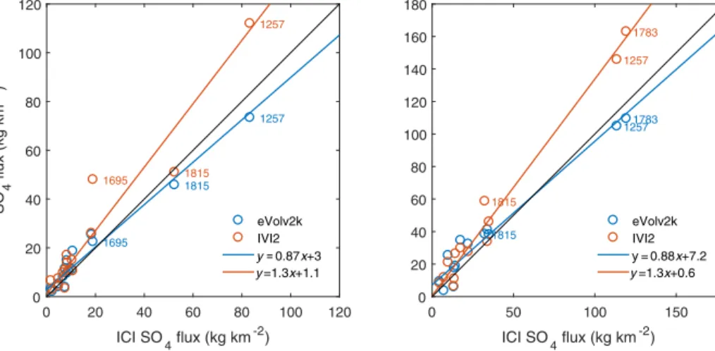
Greenland and Antarctic composite sulfate fluxes from eVolv2k are compared to composites from the IVI2 (Gao et al., 2008) and ICI (Crowley and Unterman, 2013) reconstructions in Fig. 1. For this comparison, we have fo- cused on unambiguous matches between the three sets of composites between ∼1590 and 2000, also including the 1257/8 Samalas signal, listed in Table S2. Flux composites for eVolv2k and the IVI2 datasets are plotted against the ICI reconstruction in Fig. 1.

The eVolv2k composite fluxes show rather close agreement with the values reported by ICI. Linear fits of the eVolv2k vs. ICI composite fluxes were computed using the OLS bisector method (Isobe et al., 1990), resulting in slopes of 0.89±0.14 for Greenland and 0.87±0.12 for Antarc- tica. On the other hand, the IVI2 flux values show a significant bias compared to ICI, with a slope of 1.33±0.14 for Greenland and 1.30±0.26 for Antarctica. Fits of the IVI2 fluxes against the eVolv2k fluxes (not shown) result in bias estimates of 1.49±0.21 for Greenland and 1.50±0.28 for Antarctica.

(10)

0 20 40 60 80 100 120 ICI SO₄ flux (kg km^-2)

0 20 40 60 80 100 120

SO4 flux (kg km-2 )

Antarctica

1257 1257

1815 1815

1695 1695

eVolv2k IVI2 y=0.87x+3 y=1.3x+1.1

0 50 100 150

ICI SO₄ flux (kg km^-2) 0

20 40 60 80 100 120 140 160

180 Greenland/NH

1783 1783

1257 1257

1815 1815

eVolv2k IVI2 y= 0.88x+7.2 y=1.3x+0.6

Figure 1.Composite sulfate fluxes derived from ice cores for (left) Antarctica and (right) Greenland (or NH). Values from the eVolv2k (this work) and IVI2 (Gao et al., 2008) reconstructions are plotted vs. composite values from the ICI reconstruction (Crowley and Unterman, 2013) for event matches defined in Table S2. Linear fits to the scatter plots are included, with best fit slopes and intercepts as included in the legends.

59.3

-500 -450 -400 -350 -300 -250 -200 -150 -100 -50 0

0 20 40

VSSI (Tg [S])

0 50 100 150 200 250 300 350 400 450 500

0 20 40

VSSI (Tg [S])

500 550 600 650 700 750 800 850 900 950 1000

0 20 40

VSSI (Tg [S])

59.4 64.5

1000 1050 1100 1150 1200 1250 1300 1350 1400 1450 1500 0

20 40

VSSI (Tg [S])

1500 1550 1600 1650 1700 1750 1800 1850 1900 1950 2000 Year (ISO 8601)

0 20 40

VSSI (Tg [S])

IVI2 eVolv2k

Figure 2.Volcanic stratospheric sulfur injection (VSSI) from the IVI2 and eVolv2k reconstructions. Values exceeding they-axis limits are denoted as text. Years are shown using the ISO 8601 standard, which includes a year zero.

(11)

536 540

574

626 682

939

1108 1171

1182 1230

1257

1286 1276 1345

1453 1458

1600

1640 1695

1809 1783

1815

1831

1835

0 10 20 30 40 50 60 70

IVI2 VSSI (Tg [S]) 0

10 20 30 40 50 60 70

eVolv2k VSSI (Tg [S])

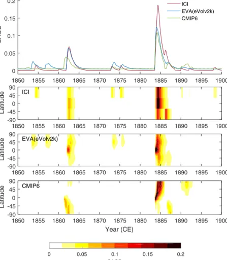
Figure 3.Scatter plot of matched eVolv2k vs. IVI2 VSSI estimates for events spanning 501–1900 CE with VSSI>10 Tg [S]. Matches are defined in Table S3, and labels show the year of each event according to the eVolv2k reconstruction. Vertical bars indicate the 1σ uncertainty in the eVolv2k VSSI estimates. The 1:1 line is shown in black, with dark and light grey shading denoting the ±10 and 33 % range around 1:1.

The apparent bias in the IVI2 fluxes compared to ICI and eVolv2k is primarily due to the reported fluxes for the largest events. When the linear fits are repeated after re- moving the largest events (1783, 1258, and 1815 for Green- land and 1258 and 1695 for Antarctica), the bias of the IVI2 fluxes compared to eVolv2k reduces to 0.90±0.34 for Green- land and 1.1±0.20 for Antarctica. For Greenland, IVI2 used a large number of supplemental ice cores in the estimates for Tambora and Laki (Clausen and Hammer, 1988; Mosley- Thompson et al., 1993), which increased the composite estimates for these events significantly compared to values originally reported using only the long-term ice core records (Gao et al., 2006). Over Antarctica, the large IVI2 composite flux for 1257 is likely a result of the very strong flux recorded by the SP01 ice core from the South Pole (Budner and Cole- Dai, 2003), which was not reproduced by another ice core record from the same site (SP04, Ferris et al., 2011) and con- sequently was not included in the AVS-2k composite (Sigl et al., 2014).

3.2 Volcanic stratospheric sulfur injection

The eVolv2k global VSSI time series is shown in Fig. 2 in comparison to the values from the IVI2 reconstruction. Over the 1500–1900 time period, the two reconstructions are very

similar in terms of the timing and magnitude of most events, including Tambora (1815) and Laki (1783). The eVolv2k VSSI estimates for Huyanaputia (1600), Parker (1640), and the unidentified eruption of 1809 are slightly larger than those of IVI2.

Within the 1000–1500 CE time period, the two reconstructions agree reasonably well in terms of the timing and magnitude of the great 1257 Samalas eruption and the eruptions of 1276 and 1286. A major difference between the reconstructions is the timing of the great mid-15th century eruption, which differs by 6 years. Before∼1250 CE, there is a notable shift in the timing of events, reaching about 6 years, and most events are of a somewhat larger magnitude in the eVolv2k reconstruction. Between 500 and 1000 CE, there is very little correlation between the two reconstructions. The eVolv2k reconstruction contains strong VSSI events, including events at 540, 574, 682, and 1108 CE, which are missing or largely underestimated in the IVI2 reconstruction. Of particular note, the eVolv2k reconstruction includes a sequence of very large eruptions in the sixth century, including a NH extratropical eruption in 536 CE and tropical eruptions in 540 and 574 CE, which is consistent with timings inferred in earlier studies (Baillie, 2008; Baillie and McAneney, 2015;

Toohey et al., 2016a) and confirmed by Sigl et al. (2015), with VSSI magnitudes 25–30 % larger than estimated by Toohey et al. (2016a). The extension of VSSI estimates back to 500 BCE reveals two large events: a Samalas-magnitude injection in 426 BCE and an event of∼40 Tg sulfur (30 % greater than Tambora) in 44 BCE.

Global VSSI magnitudes for the major events common to the eVolv2k and IVI2 datasets over the 500–1900 CE period are compared in more detail in Fig. 3. Major events were defined here as those with VSSI values greater than 10 Tg[S].

Lists were compiled of major events from both datasets, and matches between the two datasets were found based on coincidence in time (Table S3), allowing for a drift in time in the early portion of the overlap period consistent with recent updates to the ice core dating (Sigl et al., 2015). If no match was found for a strong event in one dataset, a VSSI value of 0 was specified for the other dataset.

VSSI estimates from eVolv2k and IVI2 for many of the largest events, including the 1257, 1783, and 1815 events, agree to ∼10 % (Fig. 3). This agreement reflects compen- sation between changes in the ice core sulfate flux composites used in the two reconstructions (see Fig. 1) and the 33 % increase in effective transfer function used in the construction of eVolv2k. If the 1452 event from IVI2 was matched to the 1458 event of eVolv2k, they would also agree to within 10 %, yet this agreement is largely coincidental, since the IVI2 value is based on combining values from two likely dis- parate events in 1452 and 1458 (Cole-Dai et al., 2013; Plum- mer et al., 2012; Sigl et al., 2013). A handful of other smaller events agree between the two datasets to within 33 %, including events in 536, 1182, 1276, 1286, and 1835. Five events (1230, 1171, 1600, 1640, and 1809 CE) have VSSI values

(12)

-500 0 500 1000 1500 2000 0

0.5 1 1.5

Mean VSSI (Tg [S] yr-1 )

eVolv2k IVI2

-500 0 500 1000 1500 2000

Year (ISO 8601) 0

5 10 15

Events (100 yr)-1

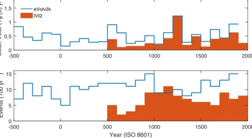
Figure 4.(a)Centennial mean volcanic stratospheric sulfur injections (VSSI) from the IVI2 and eVolv2k reconstructions.(b)The number of volcanic events per century included in the eVolv2k and IVI2 reconstructions. Years are shown using the ISO 8601 standard, which includes a year zero.

-500 -450 -400 -350 -300 -250 -200 -150 -100 -50 0

0 0.2 0.4

SAOD

0 50 100 150 200 250 300 350 400 450 500

0 0.2 0.4

SAOD

500 550 600 650 700 750 800 850 900 950 1000

0 0.2 0.4

SAOD

10000 1050 1100 1150 1200 1250 1300 1350 1400 1450 1500 0.2

0.4

SAOD

1500 1550 1600 1650 1700 1750 1800 1850 1900 1950 2000

Year (ISO 8601) 0

0.2 0.4

SAOD

EVA(eVolv2k) ICI

Figure 5.Global mean annual mean stratospheric aerosol optical depth (SAOD) from the EVA(eVolv2k) and ICI reconstructions. Years are shown using the ISO 8601 standard, which includes a year zero.

(13)

817 939

970 11711108

1182

1230

1257

1276 1345 1286

1458

1600 1640

1673

1695

1783 1809

1815

1831 1835 1883

0 0.1 0.2 0.3 0.4 0.5 0.6 0.7 0.8 0.9 1

ICI cum. glob. mean SAOD (yr) 0

0.1 0.2 0.3 0.4 0.5 0.6 0.7 0.8 0.9 1

EVA(eVolv2k) cum. glob. mean SAOD (yr)

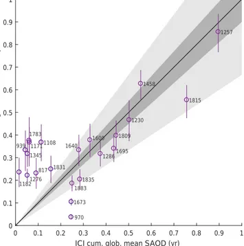
Figure 6.Scatter plot of matched EVA(eVolv2k) vs. ICI estimates of 3-year cumulative global mean SAOD for events with values greater than 0.2. Matches are defined in Table S4. Labels show the eVolv2k date of each event. Vertical bars indicate the 1σuncertainty in the EVA(eVolv2k) SAOD estimates. The 1:1 line is shown in black, with dark and light grey shading denoting the±10 and 33 % range around 1:1.

33–40 % larger in eVolv2k, representing the impact of the increased transfer functions on similar ice sheet composite fluxes. Around 10 events in eVolv2k have VSSI values significantly more than 33 % larger than in the IVI2 reconstruction. Some of these events appear to be missing (682, 1108) or significantly underestimated (540, 574, 626, 939) in IVI2, likely due to a lack of synchronisation of the underlying ice core records. Relative increases of 33–60 % for other events (e.g. 1695 and 1831) reflect in part the identification of bipolar ice core signals and therefore the assignment of a tropical source for the eruption rather than an extratropical source assumed by IVI2.

Estimated random uncertainties in the VSSI values are dis- played as vertical error bars in Fig. 3. Uncertainties for VSSI greater than 20 Tg[S]range from about 15 to 30 % (Fig. S6).

Due to relatively uniform sulfate fluxes over the Greenland and Antarctica ice core samples, VSSI estimates for the 1458 event and Tambora (1815) are among the most tightly constrained, with uncertainties of 15 and 16 %, respectively. The VSSI uncertainty for Samalas (1257) is 18 %, while the large events of 540 CE and Laki (1783) have larger uncertainties, with estimated values of 24 and 34 %, respectively.

Centennial-scale variations in the eVolv2k and IVI2 VSSI reconstructions are shown in Fig. 4. Centennial average VSSI values (Fig. 4a) are dominated by the largest events: max-

imum centennial averages occur in the 6th, 13th, and 19th centuries, which together contain 7 of the top 20 VSSI events of the eVolv2k dataset (Table 2). Minimum centennial mean VSSI is found during a “Roman Quiet Period” in the first century CE, with a mean value of about 0.1 Tg[S]yr⁻¹, a full order of magnitude less than that of the maximum century (1200–1300 CE) and less than one-third of the long-term average. The century with the second lowest level of volcanism is 1000–1100 CE, corresponding with the “Medieval Quiet Period” (Bradley et al., 2016). Compared to IVI2, eVolv2k VSSI averages are larger for all centuries, with large differences occurring near the beginning of the period of overlap (e.g. the 6th, 7th, and 10th centuries) but also in the more recent centuries (e.g. 17th and 19th centuries). The eVolv2k reconstruction also contains generally more events than that of IVI2 (Fig. 4b), with an average of 10.6 events per century compared to 6.7 events per century in the IVI2 dataset. The centennial event frequency in eVolv2k is also slightly more uniform with time, with a coefficient of variation of 0.24, compared to 0.37 for IVI2. The largest increase in the number of events identified in the eVolv2k database compared to IVI2 is in the years 500–1000 CE when eVolv2k includes 12.0 events per century compared to 5.5 events per century in IVI2.

3.3 Stratospheric aerosol optical depth

Time series of global mean SAOD from the EVA(eVolv2k) and ICI reconstructions are shown in Fig. 5 (zonal mean SAOD is shown for the full EVA(eVolv2k) reconstruction in Fig. S7). Similar to the VSSI comparisons, the timing and magnitudes of major SAOD perturbations in the two reconstructions are similar from 1250 to 1900 CE and significantly different before around 1200 CE.

A comparison of the magnitude of matched strong events in the eVolv2k and ICI SAOD reconstructions (Table S4) is shown in Fig. 6. Maximum values of 3-year cumulative SAOD are compared to reduce differences due to the different temporal evolutions or assumed starting dates of events in the two reconstructions. Most of the largest SAOD events agree to within 33 %, including the 1230, 1257, 1458, 1600, 1640, 1809, and 1815 events. Tambora is a notable case, with EVA(eVolv2k) cumulative SAOD approximately 25 % smaller than that of the ICI reconstruction. Laki (1783) and other NH extratropical eruptions (e.g. 939, 1182) have much larger SAOD in the eVolv2k reconstruction, a result of not applying a correction for effusive tropospheric eruptions as done in the ICI. Other apparent outliers can be understood to result from the inclusion of the then unsynchronised Plateau Remote and Taylor Dome ice cores in the ICI reconstruction.

Contributing 40–50 % weight to the mean Antarctic SO₄flux composite before 1200 CE, the unsynchronised series from these two ice cores generally reduced the mean sulfate values for real volcanic events while falsely generating apparent volcanic signals not observed by those ice cores that had