D DAVID PUBLISHING

(1)

doi:10.17265/2162-5298/2016.07.002

Observed Suspended Sediment Dynamics during a Tidal Cycle above Submerged Asymmetric Compound Sand Waves

Ingo Hennings and Dagmar Herbers

Department of Ocean Circulation and Climate Dynamics, GEOMAR Helmholtz Centre for Ocean Research Kiel, Kiel 24148, Germany

Abstract: The data from Acoustic Doppler Current Profiler (ADCP) of the three-dimensional current-field, echo intensity, modulation of Suspended Sediment Concentration (SSC), and related water levels and wind velocities have been analyzed as a function of water depth above submerged asymmetric compound sand waves during a tidal cycle in the Lister Tief of the German Bight in the North Sea.

Signatures of vertical current component, echo intensities and calculated SSC modulations in the water column depend strongly on wind and current velocity. Bursts of vertical current component and echo intensity are triggered by sand waves itself as well as by superimposed megaripples due to current wave interaction at high current



1.0 ms^-1 and wind speeds



10.0 ms^-1, preferably of opposite directions, measured at high spatial resolution. The magnitude of currents and SSC modulations during ebb and flood tidal current phases are only weakly time dependent, whereas the local magnitudes of these parameters are variable in space above the sand waves. Some hydrodynamic parameters are further investigated and analyzed, showing a consistence of ADCP measurements in the applied theory.

Key words: Acoustic Doppler Current Profiler, suspended sediment concentration, asymmetric compound sand wave, dynamic buoyancy density, action density.

1. Introduction

^

Ocean color and its transparency are related to turbidity caused by substances in water like organic and inorganic material. One of the essential climate variables (ECV) is ocean color. However, this implies the correct interpretation of observed water quality parameters. Measurements of wavelength variations of the beam attenuation coefficient provide information of the major constituents of the water influencing its color. Ocean color is also important for technical applications and operations, because the utilization of new remote sensing technologies for hydrographic purposes such as airborne light detection and ranging (LIDAR) bathymetry (ALB) systems for shallow coastal surveys depends strongly on turbidity of the water column. Worldwide, ocean dynamics such as

Corresponding author: Ingo Hennings, Ph.D., main research field: ocean remote sensing.

water circulation and global current systems, as well as water constituents influence the formation, kind and localization of deposits. It was shown [1] that it had failed to find a strong link between diatom chlorophyll concentration in the upper water column at the ocean surface and diatom ooze occurrence at the seafloor.

This implies, contrary to a widely held view, that diatom oozes are not a reliable proxy for surface productivity.

In 1953, the influence of suspended and dissolved matter on the transparency of sea water was already extensively investigated [2]. Influences of phytoplankton pigments on the color of sea water were presented [3]. It is well known that a strong coherence exists between fluctuations of turbidity, phytoplankton concentration, and SSC induced by disturbances of tidal current velocities. Linkages between turbidity distributions and density stratification were reported [4] and the relationship

D

DAVID PUBLISHING

(2)

Observed Suspended Sediment Dynamics during a Tidal Cycle above Submerged Asymmetric Compound Sand Waves

334

between phytoplankton, temperature stratification and turbidity features was investigated [5]. Substantial phenomena of SSC during two tidal cycles at two anchor stations in the southern North Sea were described [6]. It was shown that a phase shift of 30-45 minutes had happened between turbidity and current velocity maximum. Relations between turbidity and water temperature stratification of a selected North-South transect in the North Sea acquired in August 1953 were summarized [7]. A summary of extinction measurements made by the German Hydrographic Institute (now: Federal Maritime and Hydrographic Agency (BSH)), Hamburg, Germany, during the decade after the Second World War was published [8]. Different factors such as water masses, phytoplankton production, bathymetry, wave action, tidal stream and bottom sediment affecting turbidity in the southern North Sea were also discussed [9].

Measurements of SSC close to the shore derived by optical and acoustic backscatter sensors were described [10]. Spatial variability in SSC, over distance scales of less than 15 cm, related to vortex ejection from bedforms like surface wave-formed ripples. Erosion of sediments at the sea bottom associated with turbidity clouds developed under anti-cyclonic rotations in the water column in shallow waters in the German Bight of the North Sea at weather conditions with strong westerly winds was reported [11]. Hamilton et al. [12]

aimed to provide an introduction using acoustic backscatter techniques in monitoring SSC profiles, particularly for the difficult regime of cohesive suspensions. In-situ observations in the past showed that submerged sand waves and internal waves associated with vertical current components can be sources of enhanced SSC in the water column above sea bottom topography. Often, such SSC features can come up to the water surface in shallow tidal seas of the ocean. Hennings et al. [13] showed that in a stratified two water layer system, simultaneous reductions in the near-surface water temperature and beam transmittance have been recorded, whereas fluorescence data are

increased above sand waves. Quaresma et al. [14]

published their results concerning that the passage of each nonlinear internal wave is pumping near bottom suspended sediment to levels above the bottom nepheloid layer, therefore contributing to the measured short-period echo intensity increase in the vertical region. A good linear relationship between water depth and total suspended sediment (TSM) data derived from Moderate Resolution Imaging Spectroradiometer (MODIS) measurements above sand ridges in the southern Yellow Sea was found [15]. The TSM concentration was proportional to the inverse water depth; high TSM concentrations were located above shallow parts of sand ridges. It was shown [16] that strong currents flowing over steep bottom topography are able to stir up the sediments to form both a general continuum of SSC and localized pulses of higher SSC in the vicinity of the causative bed feature itself. These observations were in agreement with the basics on dynamics of the ocean circular vortex and wave motions [17, 18]. Tide-dependent variations in the formation and dynamics of suspended sediment patterns coupled to mean flow and turbulence above asymmetric bedforms were examined [19]. A decrease in water clarity of the southern and central North Sea was reported [20]. The authors concluded that changes in water clarity were more likely driven by an increase in SSC.

The primary intention of this paper is to investigate the effect of wind speed and direction as well as current speed over ground of the measuring platform on signatures of vertical current component

w

, echo intensity

E

₃ and SSC modulation

log    c / c

₀



₃



above submerged asymmetric compound sand waves during a tidal cycle. Another central question is whether localized pulses of higher SSC in the vicinity of stirring sea bed features depending on wind velocity and spatial resolution rise high enough in the water column and become resolvable to the extent that they create distinct signatures in space-borne optical

(3)

imagery. Hydrodynamic parameters such as dynamic buoyancy density, total energy density and action density due to semi-diurnal M2 tide motion are investigated, analyzed and simulated for verifying Acoustic Doppler Current Profiler (ADCP) measurements.

Two examples of ocean color phenomena are briefly introduced in part 2.1. The methods and measurements conducted during a tidal cycle above asymmetric compound sand waves in the Lister Tief and time dependent measurements of vertical water depth averaged data are described and analyzed in part 2.2 and parts 2.2.1-2.7.2, respectively. Part 2.4 presents the simple theory of hydrodynamics which are associated with sand waves. Results, characteristics and discussion of simulated physical and oceanographic parameters are presented in parts 3.1-3.2. Finally, the conclusions are outlined in part 4.

2. Material and Methods

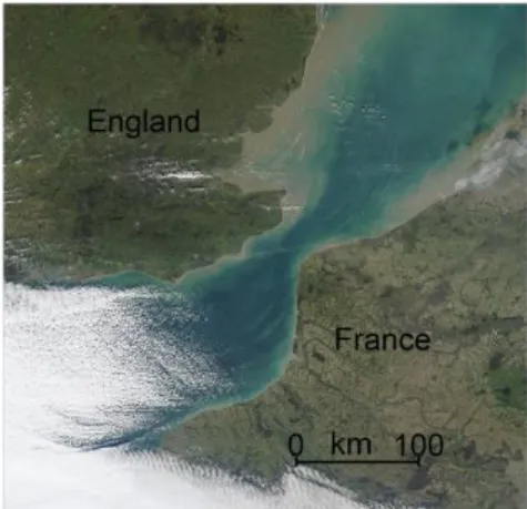
2.1 MODIS Satellite and Handheld Camera Images To illustrate some turbidity features of coastal waters, a synoptic view of a satellite image and a local view of a handheld camera picture are shown. An example of ocean color features due to tidal motion and wind-wave action is presented in Fig. 1. This true color of Terra-MODIS satellite image shows the Strait of Dover between England and France and the coverage of two-thirds of the image shown in Fig. 1 is marked by black broken lines in Fig. 3. The acquisition time of the Terra-MODIS scene was at 11:17 UTC on 9 December 2002, 3 hours and 15 minutes before high water at Dover (location see Fig.

3), England, during ebb tidal phase with southwesterly tidal current directions. Wind gusts to 21 ms^-1 from east-southeasterly directions continuing this day affecting coastal areas of East England. Spatial resolution of the satellite image is 250 m. Green color of turbidity signatures associated with submerged tidal current ridges are visible in open coastal waters and brown color of turbidity or high suspended sediment

Fig. 1 Terra-MODIS satellite image of the Strait of Dover between United Kingdom and France (National Aeronautics and Space Administration (NASA), File:

England.A2002343, 1115.250m.jpg) acquired at 11:17 UTC on 9 December 2002 with a spatial resolution of 250 m.

Green color of turbidity signatures manifest submerged tidal current ridges in open coastal waters and brown color of turbidity indicates high suspended sediment concentrations near the coasts. White color of clouds covers the lower left part of the image.

Fig. 2 Handheld camera image views the sea surface of Hohwacht Bight, a part of Kiel Bight, at the German coast of the Baltic Sea. The location is indicated by a green circle in Fig. 3. Color contrast is the most distinctive signature of the water surface which expresses a turbidity front. Blue color shows the open ocean and green/brown color is associated with near coastal waters.

concentrations (SSCs) are identified near the coasts.

White color, which represents clouds, covers mainly the lower left quarter of the scene.

The image shown in Fig. 2 is an example of ocean color signatures at the sea surface due to wind-wave action of Hohwacht Bight at the German coast of the

(4)

336

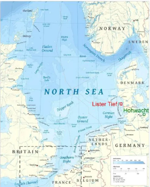
Fig. 3 The image presents an overview of the North Sea. The study area of the Lister Tief located northerly of the island of Sylt in the German Bight of the North Sea shown in Fig. 4 is marked by a red circle. In addition, two-thirds of the coverage of the Terra-MODIS satellite image presented in Fig. 1 is indicated by broken black lines and the location of Hohwacht Bight shown in Fig. 2 is marked by a green circle.

Baltic Sea. Its location is indicated by a green circle in Fig. 3. The image presented in Fig. 2 was acquired from the shore at 09:20 UTC on 08 February 2015.

The mean wind speed was 10 ms^-1 and the mean wind direction was from 339° (north-northeasterly). Winds were gusting up to a maximum of 20.8 ms^-1. The most distinctive signature of the water surface is the turbidity front expressed by the color contrast. The open ocean has a dark blue color whereas the near coastal waters are green/brown. The green/brown band of the electromagnetic spectrum is sensitive to

scattering from an ensemble averaged size of sand grain suspended in the water column. Near water surface signatures are likely detectable in the optical and visible part of the electromagnetic spectrum by air- and space-borne remote sensing systems as shown in Fig. 1 caused by strong surface wave interactions at sea bottom in the coastal zone. Due to strong wave action at the sea bottom, sediments were moved upwards in the upper layer of the water column. The turbidity front corresponds approximately with the 15 m water depth contour line.

(5)

2.2 Measurements Conducted during a Tidal Cycle in the Liser Tief

The study area of the Lister Tief is a tidal inlet of the German Bight in the North Sea bounded by the islands of Sylt to the South and Rømø to the North.

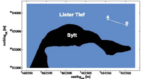
Location of the Lister Tief is shown in Fig. 3 and marked by a red circle. The positions of analyzed runs along transect AB in the Lister Tief are presented in Fig. 4. Tide gauge station List is located 4.8 km southerly of transect AB. The seabed morphology in the Lister Tief is a complex configuration of continuously changing different bed forms. The submerged compound sand waves investigated in this study are four-dimensional in space and time.

Small-scale as well as megaripples are superimposed on sand waves as presented here and already discussed in [21, 22]. Analyzed flood dominated sand waves have stoss slopes of the order of 2° and lee slopes up to 31°. High resolution 2 D seismic (sparker and Chirp III) profiles have been acquired during 2005-2009 around the northern part of Sylt [23]. These data revealed bedform configurations and sub-bottom structures to a depth of 75-100 meters below seafloor (mbsf) for the sparker data and ca. 20 mbsf for the Chirp III data and thus added valuable information to previously obtained sidescan seabed registrations.

The measurement configuration and sensor

parameters which are used during the Operational Radar and Optical Mapping (OROMA) in monitoring hydrodynamic, morphodynamic and environmental parameters for coastal management project from on board the research vessel (R/V) Ludwig Prandtl are introduced in Ref. [16]. Water levels measured at tide gauge station List, wind and current velocities, vertical current components

w

, echo intensities

E

₃

of fore beam No. 3 measured by ADCP and calculated SSC modulations expressed as

log    c / c

₀



₃



of beam No. 3 as a function of water depths are presented. The constant SSC equilibrium term is defined by

c

₀ and

 c

is the time-dependent perturbation term of the local SSC

c

. All parameters are measured and calculated over submerged asymmetric compound sand waves at the sea bottom during several runs along transect AB. The measurements during runs 48 and 51 are shown in Figs. 5a-e and 7a-e for ebb tidal current phase and those during runs 64 and 65 are shown in Figs. 9a-e and 11a-e for flood tidal current phase. The duration of the measurement time is indicated by a vertical black line in Figs. 5a, 7a, 9a and 11a, respectively.

Each run has been rotated by an angle of 19° in order to direct the current component

u

perpendicular to the sand wave crest. Hence, the

v

-component of the current field is minimized and can be neglected as a

Fig. 4 Positions of runs along transect AB in the Lister Tief where ADCP measurements and other meteorological and oceanic parameters are acquired from on board R/V Ludwig Prandtl.

(6)

338

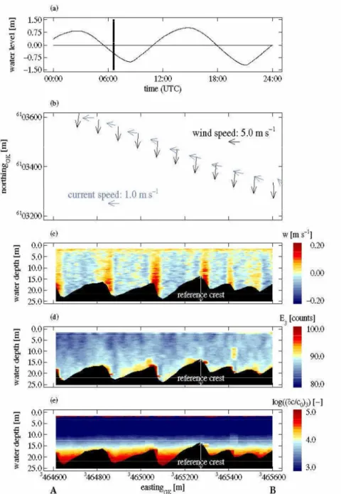
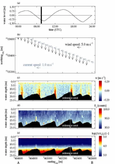
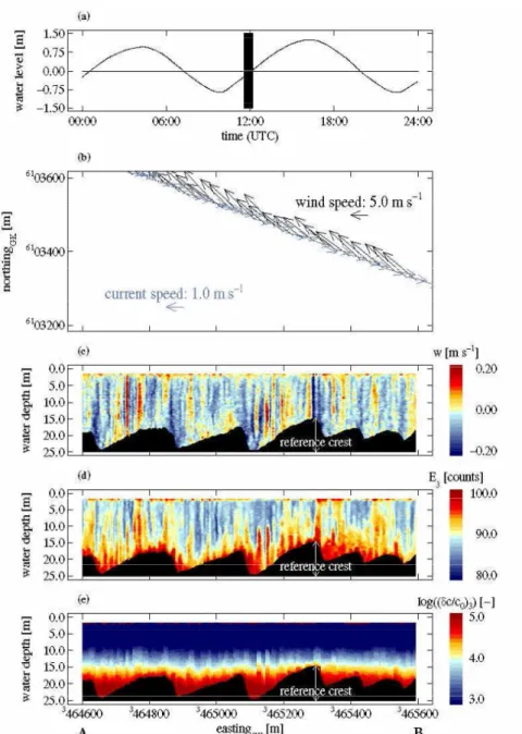
Fig. 5 Analyzed data of ADCP of fore beam No. 3 as a function of position and water depth above asymmetric sand waves of run 48 along transect AB indicated in Fig. 4 during ebb tidal phase at 0633-0641 UTC on 10 August 2002; (a) time series of water levels measured at the tide gauge station List; (b) wind and current velocities, the two horizontal arrow-scales indicate a wind speed of 5.0 ms^-1 and a current speed of 1.0 ms^-1, respectively; along-track presentations of (c) vertical current component

w

of the three-dimensional current field; (d) echo intensity

E

₃ and (e) calculated SSC modulation

 

 /

₀ ₃



log  c c

. The timing of the measurement is marked by a vertical black line in a). The position of the reference crest is indicated at the highest sand wave crest of the run.

first approximation. The rotation point is marked at the highest sand wave crest along the profile named as reference crest, shown in Figs. 5c-e, 7c-e, 9c-e and 11c-e, respectively. The current vectors shown in Figs.

5b, 7b, 9b and 11b are water depth averaged velocity

values. Time interval of both, wind and current velocity arrows, is 30 s. Especially, Figs. 5d, 6, 7d, 8, 9d, 10, 11d and 12 illustrate the resuspension expressed by

E

₃ in progress at ebb and flood tides for different wind conditions.

(7)

2.2.1 Measurements of Run 48 during Ebb Tidal Phase

The acquisition time of the measurements shown in Figs. 5a-e was during ebb tidal phase at 0633-0641 UTC on 10 August 2002, after previous high water at station List at 0226 UTC on 10 August 2002. Wind speeds between 5.8 ms^-1 and 7.5 ms^-1 from northerly directions were measured (Fig. 5b). The mean current speed u was 1.0 ms^-1 with a mean current direction of 283°. It is shown in Fig. 5b that the angle between the current and wind direction is 90°. The up- and downward components

w

of the current velocity (Fig. 5c) are regularly distributed in the water column above stoss and lee slopes of sand waves. Enhanced

echo intensity counts

E

₃ are shown close to the sea bottom of sand waves and afterwards reduced intensity counts

E

₃ are distributed in the upper 15 m of the water column. The SSC modulations

 

 /

₀ ₃



log  c c

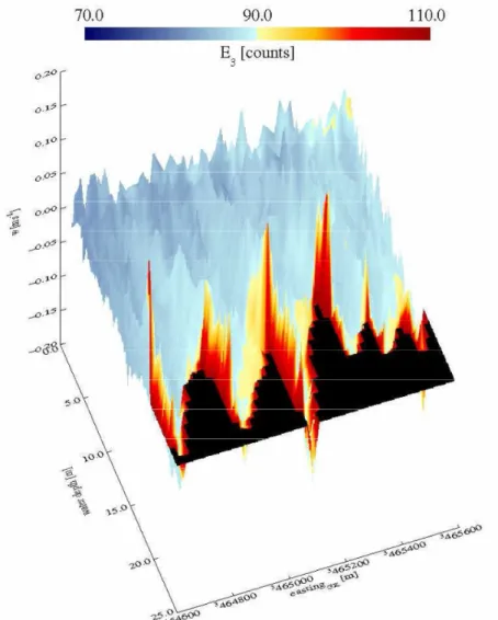
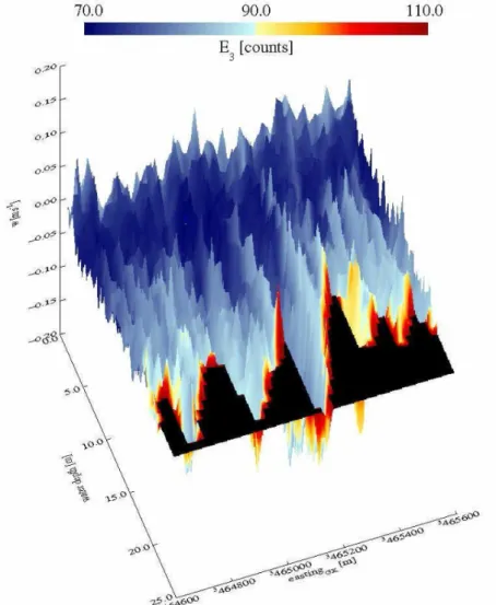
(Fig. 5e) show enhanced values close to the sea bottom up to a height of 8 m at the troughs of sand waves. R/V Ludwig Prandtl sailed with the current direction along this run of transect AB.

The three dimensional presentation of

w

and

E

₃

as a function of position and water depth along the same run of transect AB shown in Figs. 5c-e is presented in Fig. 6. The positive and negative amplitudes of

w

(up- and downwelling) are superimposed by color

Fig. 6 Three dimensional presentation of

w

and

E

₃ (color coded) as a function of position and water depth along the same run of transect AB shown in Figs. 5c-e.

(8)

340

Fig. 7 Analyzed data of ADCP of fore beam No. 3 as a function of position and water depth above asymmetric sand waves of run 51 along transect AB indicated in Fig. 4 during ebb tidal phase at 0721-0740 UTC on 10 August 2002; (a) time series of water levels measured at the tide gauge station List; (b) wind and current velocities, the two horizontal arrow-scales indicate a wind speed of 5.0 ms^-1 and a current speed of 1.0 ms^-1, respectively; along-track presentations of (c) vertical current component

w

E

₃ and (e) calculated SSC modulation

 

 /

₀ ₃



log  c c

. The timing of the measurement is marked by a vertical blackline in (a). The position of the reference crest is indicated at the highest sand wave crest of the run.

coded values of

E

₃. If high positive amplitudes of

w

and high (red color) values of

E

₃ coincide, for example, these two parameters are proportional. It is shown in Fig. 6 that high values of

w

and

E

₃ are only observed close to the sea bottom of sand waves.

2.2.2 Measurements of Run 51 during Ebb Tidal Phase

The acquisition time of the measurements shown in Figs. 7a-e was during ebb tidal phase at 0721-0740 UTC on 10 August 2002, after previous high water at

(9)

station List at 0226 UTC on 10 August 2002. Wind speeds between 6.7 ms^-1 and 7.5 ms^-1 from northerly direction were measured (Fig. 7b). A mean current speed u ^{= 0.7 ms}^-1 and a mean current direction of 281° were calculated. The angle between current and wind direction is 90° and is shown in Fig. 7b. The up- and downward components

w

of the current velocity (Fig. 7c) are regularly distributed in the water column above stoss and lee slopes of sand waves.

Echo intensity counts

E

₃ are reduced in the water column and close to the sea bottom of sand waves because the observation time of the run finished 45 minutes before low tide at station List. The SSC modulations

log    c / c

₀



₃



(Fig. 7e) show enhanced values only close to the sea bottom up to a

height of 9 m at the troughs of sand waves. R/V Ludwig Prandtl sailed against the current direction along this run of transect AB.

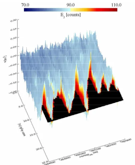
The three-dimensional presentation of

w

and

E

₃

as a function of position and water depth along the same run of transect AB shown in Figs. 7c-e is presented in Fig. 8. It is shown in Fig. 8 that high values of

w

and

E

₃ are only observed close to the sea bottom of sand waves.

2.2.3 Measurements of Run 64 during Flood Tidal Phase

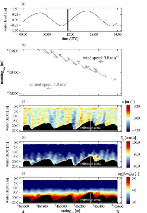
The acquisition time of the measurements shown in Figs. 9a-e was during flood tidal phase at 1116-1128 UTC on 12 August 2002, after previous low water at station List at 0957 UTC on 12 August 2002.

Wind speeds between 9.2 ms^-1 and 10.0 ms^-1 from

w

and E₃ (color coded) as a function of position and water depth along the same run of transect AB shown in Figs. 7c-e.

(10)

342

Fig. 9 Analyzed data of ADCP of fore beam No. 3 as a function of position and water depth over asymmetric sand waves of run 64 along transect AB indicated in Fig. 4 during flood tidal phase at 1116-1128 UTC on 12 August 2002; (a) time series of water levels measured at the tide gauge station List; (b) wind and current velocities, the two horizontal arrow-scales indicate a wind speed of 5.0 ms^-1 and a current speed of 1.0 ms^-1, respectively; along-track presentation of (c) vertical current component

w

E

₃ and (e) calculated SSC modulation of

 

 /

₀ ₃



log  c c

. The timing of the measurement is marked by a vertical black line in (a). The position of the reference crest is indicated at the highest sand wave crest of the run.

southeasterly were measured (Fig. 9b). A mean current speed u = 1.0 ms^-1 and a mean current direction of 106° were calculated. The current and wind direction are opposite (Fig. 9b). The up- and downward components

w

of the current velocity,

presented in Fig. 9c, vary between 0.2 ms^-1 and -0.2 ms^-1. There is a correlation between up-/downwelling features of

w

and stoss/lee slopes of sand waves.

Enhanced echo intensity counts E₃, shown in Fig. 9d, are localized close to the bottom of sand waves and

(11)

growing as bursts above sand waves. Enhanced SSC modulations

log    c / c

₀



₃



(Fig. 9e) are present at the sea bottom up to a height of 12 m above sand waves due to higher wind speeds causing stronger wave current interaction. R/V Ludwig Prandtl sailed with the current direction along this run of transect AB.

The three-dimensional visualization of

w

and

E

₃

as a function of position and water depth along the same run of transect AB shown in Figs. 9c-e is presented in Fig. 10. The positive and negative amplitudes of

w

(up- and downwelling) are again superimposed by color coded values of

E

₃. Well defined bursts of enhanced

E

₃ associated with high

amplitudes of

w

are developed in the water column above the gentle slopes of sand waves.

2.2.4 Measurements of Run 65 during Flood Tidal Phase

The acquisition time of the measurements shown in Figs. 11a-e was during flood tidal phase at 1133-1210 UTC on 12 August 2002, after previous low water at station List at 0957 UTC on 12 August 2002. Wind speeds between 11.7 ms^-1 and 13.3 ms^-1 from southeasterly direction were measured. A mean current speed u ^{= 1.0 ms}^-1 and a mean current direction of 107° have been monitored. The current and wind direction are almost opposite (Fig. 11b). The up- and downward components

w

of the current velocity (Fig. 11c) with values between 0.2 ms^-1 and

w

and

E

(12)

344

Fig. 11 Analyzed data of ADCP of fore beam No. 3 as a function of position and water depth over asymmetric sand waves of run 65 along transect AB indicated in Fig. 4 during flood tidal phase at 1133-1210 UTC on 12 August 2002; (a) time series of water levels measured at the tide gauge station List; (b) wind and current velocities, the two horizontal arrow-scales indicate a wind speed of 5.0 ms^-1 and a current speed of 1.0 ms^-1, respectively); along-track presentation of (c) vertical current component

w

E

₃ and (e) calculated SSC modulation of

 

 /

₀ ₃



log  c c

. The timing of the measurement is marked by a vertical black line in (a). The position of the reference crest is indicated at the highest sand wave crest of the run.

-0.2 ms^-1 are distributed as a vast number of signatures above sand waves. There is no definite relation anymore between up-/downwelling structures of

w

and stoss/lee slopes of sand waves. Enhanced echo intensity counts

E

₃, shown in Fig. 11d, are localized close to the bottom of sand waves and

growing as bursts or stirring and pumping effects above sand waves close to the water surface. However, the strongest SSC modulations

^log   ^ ^c ^/ ^c

₀



₃



^(Fig.

11e) are shown as bursts at the sea bottom of sand waves. The inhomogeneous distributions of

w

,

E

₃

(13)

and

^log   ^ ^c ^/ ^c

₀



₃



in relation to the stoss and lee slopes of sand waves are caused by high wind speeds, because wind and current direction are almost opposite. R/V Ludwig Prandtl sailed against the current direction along this run of transect AB.

Therefore, the acquisition time of 37 minutes was longer than that of the other runs. On the other hand, the spatial resolution of the different parameters visualized in Figs. 11b-e is increased as sailing against the current. The bursts of

w

and

E

₃, shown in Figs.

11c-d, indicate episodic resuspension events which may be triggered by superimposed megaripples developed on sand waves by enhanced current wave interaction at high current and wind speeds of

opposite directions, respectively.

A three dimensional presentation of

w

and

E

₃

as a function of position and water depth along the same run of transect AB shown in Figs. 11c-e is presented in Fig. 12. The positive and negative values of

w

(up- and downwelling) are again superimposed by color coded values of

E

₃. High values of

E

₃ are related to high amplitudes of

w

more or less in the whole water column.

2.3 Time Dependent Measurements of Vertical Water Depth Averaged Data

All parameters shown in Figs. 13c-f and 14c-f are time series of vertically water depth averaged values as a function of space of five selected single runs

w

and

E

(14)

346

Fig. 13 (a) Time series of water level measured at tide gauge station List with acquisition times marked by Nos. 0-4 of 5 selected runs analyzed during ebb tidal current phase from B to A while the research vessel is sailing against the current direction on 10 August 2002; (b) measured wind velocities; the horizontal arrow-scale indicates a wind speed of 5.0 ms^-1; (c) time series of measured current component

u

; the east direction is marked by a red stick within the compass symbol; (d) time series of echo intensity

E

₃ of fore beam No. 3 measured by the ADCP; (e) time series of measured vertical current component

w

; (f) time series of calculated SSC modulation expressed as

log    c / c

₀



₃



of beam No. 3; and (g)-(h) measured water depth profile of asymmetric submerged sand waves on the sea bed along transect AB (for location see Fig. 4).

during ebb tidal current phase while the research vessel is sailing against and with the current direction, respectively.

2.3.1 Research Vessel is Sailing against Current Direction during Ebb Tide

The water level measured at the tide gauge station List with the acquisition times of analyzed runs while the research vessel is sailing against current direction

during ebb tidal current phase, wind velocities, current component

u

(east direction, indicated by a compass symbol with a red stick in Fig. 13c), echo intensity

E

3 of fore beam No. 3 measured by ADCP, vertical current component

w

, calculated SSC modulations expressed as

^log   ^ ^c ^/ ^c

₀



₃



of beam No. 3 over submerged asymmetric sand waves on the sea bottom

(15)

of transect AB are shown in Figs. 13a-h. The parameters

u

,

E

₃,

w

and

log    c / c

₀



₃



were observed between 0516 UTC and 0740 UTC before low water at 0829 UTC on 10 August 2002 at tide gauge station List (acquisition times see Fig. 13a).

Wind speeds between 5.8 ms^-1 and 7.5 ms^-1 from northerly directions were measured (Fig. 13b).

Negatively, enhanced and positive values of

u

,

E

₃

and

w

, respectively, show phase relationships with sand wave crests of the sea bed. In contrast, enhanced

 

 /

₀ ₃



log  c c

shows a phase relationship with the sand wave troughs of the sea bed. The parameters

u

,

w

and

log    c / c

₀



₃



are only weakly time dependent. All signatures of

u

,

E

₃ ,

w

and

 

 /

₀ ₃



log  c c

, respectively, show spatially dependent variations in

x

-direction above the sand waves.

2.3.2 Research Vessel is Sailing with Current Direction during Ebb Tide

The water level is measured at the tide gauge station List with the acquisition times of analyzed runs while the research vessel is sailing with the current direction during ebb tidal current phase, wind velocities, current component

u

(east direction, indicated by a compass symbol with red stick in Fig.

14c), echo intensity E₃ of fore beam No. 3 measured by ADCP, vertical current component

w

, calculated SSC modulations expressed as

 

 /

₀ ₃



log  c c

of beam No. 3 over submerged asymmetric sand waves on the sea bottom of transect AB are shown in Figs. 14a-h. The parameters

u

, E₃,

w

and

log    c / c

₀



₃



were observed between 0502 UTC and 0715 UTC before low water at 0829 UTC on 10 August 2002 at tide gauge station List (acquisition times see Fig. 14a). Wind speeds between 5.8 ms^-1 and 7.5 ms^-1 from northerly directions were

monitored (Fig. 14b).

Negatively, enhanced and positive values of

u

, E3 and

w

, respectively, show phase relationships with the sand wave crests of the sea bed. In contrast, enhanced

log    c / c

₀



₃



shows a phase relationship with the sand wave troughs of the sea bed. The parameters

u

,

w

and

log    c / c

₀



₃



are only weakly time dependent. Again, as it is shown in Fig.

13, all signatures of

u

, E₃ ,

w

and

 

 /

0 ₃



log  c c

, respectively, show spatially dependent variations in

x

-direction above the sand waves.

2.4 Theory of Hydrodynamics above Submerged Sand Waves

The focus of this part is the understanding and mathematical description of dynamic buoyancy density, total energy density, and action density above submerged asymmetric sand waves due to semi-diurnal lunar M₂ tidal motion. Simple hydrodynamic relations are applied regarding the complexity of the evolved physics. The dynamic buoyancy A~_d

in the water column of volume



^x ^y ^z



V , , with the horizontal and vertical space coordinates

x

, y and z is defined by

 

  





















b b

z a z

a d

dz u c

F

dz u c

F A

0 2 0

2

2 1 1

~





(1)

Eq. (1) can be approximated by



1



²

2 1

~ F c z u

A_d  



  _a   _b  (2) and the dynamic buoyancy density

A

_d is defined by



1



²

2

~ 1

u z c

F

A A _a

b

d d     

 



(3)

(16)

348

Fig. 14 (a) Time series of water level measured at tide gauge station List with the acquisition times marked by Nos. 0-4 of 5 selected runs analyzed during ebb tidal current phase from B to A while the research vessel is sailing with the current direction on 10 August 2002; (b) measured wind velocities; the horizontal arrow-scale indicates a wind speed of 5.0 ms^-1; (c) time series of measured current component

u

; the east direction is marked by a red stick within the compass symbol; (d) time series of echo intensity

E

₃ of fore beam No. 3 measured by the ADCP; (e) time series of measured vertical current component

w

; (f) time series of calculated SSC modulation expressed as

log    c / c

₀



₃



of beam No. 3; and (g)-(h) measured water depth profile of asymmetric submerged sand waves on the sea bed along transect AB (for location see Fig. 4).

with z_b the local water depth,



the water level, F the infinitely thin horizontal plane element,  the water density, ca the dimensionless lift coefficient,

u

the local current velocity perpendicular to the sand wave crest and

u

its vertical average. The integration has to be done from

the sea bottom

z  z

_b to the water surface

 0

 

z

in Eq. (1). The dimensionless lift coefficient

c

_a is defined for a flat plate as [24]

 





¹ ²

1 sin



 

 







 

c

a (4)

(17)

and









(5)

with



the slope angle of the stoss or lee plane of the sand wave. Both, stoss as well as lee sides of the sand wave were approximated by a flat plate.

However, here c_a was subtracted by 1 in Eqs.

(1)-(3), whereas [24] normalized c_a by 1. The reason here is that both upwelling (positive) as well as downwelling (negative) values of c_a can arise above sand waves. As a first approximation, for the downforce at the lee side of the sand wave, the negative value (downforce coefficient) of the lift coefficient c_a is used here. Kinematic molecular viscosity and roughness effects at the sea bed are neglected.

The gradient of the dynamic buoyancy density perpendicular to the sand wave crest is derived as

 

x u u x c

A

a d



 





 

 1 

(6)

The potential energy E~_p in the water column in hydrodynamic theory is defined as

 









 ^b

z

R

p F g z z dz

E

0

~





(7)

where g is the acceleration due to gravity and zR

is the reference water depth at the trough of sand wave.

The integration has to be done from the sea bottom

z

b

z 

to the water surface

z    0

. The result for E~_p is then expressed as



 



 



 _b _R _b

p F g z z z

E 2

1

~



(8)

Potential energy density Ep_becomes



 



 



 

 _R _b

b p

p g z z

z F E E

2

~ 1



(9)

and kinetic energy

E ~

_k

is given by

2 0

2

2 1 2 1

2 ~ 1

u z F

dz u F

dz u F E

b z z

k

b b





















(10)

Kinetic energy density

E

_k is derived as

2

~ 1 z u F E E

b k

k   

 



(11) Transforming Eq. (3) to

 1 

2

2 



 

a d

c u A



(12) and inserting Eq. (12) into Eq. (11), the following expression for

E

_k as a function of dynamic buoyancy density is obtained

) 1

( 



a d

k

c

E A

(13)

The total energy density E is the sum of Eqs. (9) and (13).



1



2 1

 



 



 









a d b

R k

p c

z A z

g E

E



(14)

and the action density

N

is defined by



'

N  E (15)

where



^' is the radial frequency of the semi-diurnal lunar M₂ tidal wave with

T



^'  ²



(16)

where T is the period of the semi-diurnal lunar M₂ tidal wave.

Using Eqs. (6), (14) and (15), the gradient of the action density

N

perpendicular to the sand wave crest is derived as

 

 







 



 

 



x u u x g z x

N

_b

2 1



'



(17)

(18)

350

Eq. (17) shows that the gradient of the action density caused by the semi-diurnal M₂ tidal wave is antiproportional to the slope of the sea bed

 z

_b

/  x

and proportional to the product of the vertical averaged current speed and its gradient ^u^



^^u^/^^x



^,

respectively.

Assuming that the vertical averaged current speed

u

perpendicular to the sand wave crest obeys the continuity equation

c const z

u 

_b

 

(18) and inserting Eq. (18) into Eq. (17) for

 u /  x

, the following expression is derived



 



 



 

 



b b

z u g x z x

N ²

' 2





(19)

where N/x is proportional to u² and

 

zb ^¹^.

3. Results and Discussion

3.1 Evaluation and Results of Simulations

For all simulations a sand wave length L = 220 m and a sand wave height h_c = 6 m are selected. These parameters are typical values measured in the southern part of Lister Tief (see part 2.2). Simulations of the sand wave profile with water depth

z

_b, slope of the sea bed z_b /x, vertical averaged tidal current speed

u

and its gradient

 u /  x

, respectively, dynamic buoyancy density A_d , gradient of the dynamic buoyancy density

 A

_d

/  x

, kinetic energy density

Ek, potential energy density Ep, action density

N

, and gradient of the action density

 N /  x

as a function of space variable

x

are shown in Figs.

15a-e for flood and in Figs. 16a-e for ebb tidal current phase of asymmetric flood orientated sand waves, respectively. Typical values for the spatial resolutions

x = 10 m and

 y

= 1 m, z_R = 25 m, gentle slope of sand wave



g = 2°, steep slope of sand wave



_s = 9°,



= 1020 kgm^-3,

u

= 0.7 ms^-1 at x with z_b = z_R,

u

= 0.95 ms^-1 at x = 0 m (sand wave crest), g = 9.82 ms^-2, and T = 12.42 hours are calculated or inserted by using Eqs. (1)-(19).

The sea bed profile with water depth

z

_b which defines the asymmetric sand wave in black and the slope of the sea bed z_b /x in red are shown in Figs. 15a and 16a.

The tidal current velocity

u  u

is presented in black in Fig. 15b during flood and Fig. 16b during ebb

Fig. 15 Simulations of oceanographic parameters applying Eqs. (1)-(19) for flood tidal current phase (current is directed from left to right) as a function of space variable

x

; (a) sand wave profile with water depth

z

_b in black and slope of the sea bed

 z

_b

/  x

in red; (b) tidal current velocity

u  u

(black color) and gradient of the tidal current velocity

 u /  x   u /  x

(red color); (c) dynamic buoyancy density

A

_d in black and gradient of the dynamic buoyancy density

 A

_d

/  x

in red; (d) kinetic energy density E_k in black and potential energy density Ep in red; and (e) action density

N

in black and gradient of the action density

 N /  x

^{in red.}

(19)

Fig. 16 Simulations of oceanographic parameters applying Eqs. (1)-(19) for ebb tidal current phase (current is directed from right to left) as a function of space variable

x

; (a) sand wave profile with water depth

z

_b_{in black}

and slope of the sea bed

 z

_b

/  x

in red; (b) tidal current velocity

u  u

in black and gradient of the tidal current velocity

 u /  x   u /  x

in red; (c) dynamic buoyancy density

A

_d in black and gradient of the dynamic buoyancy density

 A

_d

/  x

in red; (d) kinetic energy density

E

_k in black and potential energy density E^p_in

red; and (e) action density

N

in black and gradient of the action density

 N /  x

in red.

tidal current phases. Due to the continuity of Eq. (18),

u

acquires its maximum absolute value at the sand wave crest. The gradient of the tidal current speed

x u x

u    

 / /

is shown in red in Figs. 15b and 16b, respectively. Relative strong convergent flow -

x u 

 /

= -0.007 s^-1 can be observed at the steep slope of the sea bed during flood tidal current phase.

During ebb tidal current phase a relative strong divergence flow

 u /  x

= 0.007 s^-1 is calculated at the steep slope of the sea bed.

The dynamic buoyancy density

A

_d shown in black in Figs. 15c and 16c, respectively, strongly depends on the slope of the sea bed; a maximum positive value

A

d = 50 N (upwelling) is calculated at the gentle slope of the sea bed and a maximum negative value

A

d = -160 N (downwelling) is calculated at the steep slope of the sea bed during flood tidal current phase.

A reversal of

A

_d is obtained during ebb tidal current phase. These simulations agree with ADCP measurements of vertical positive and negative components

w

of the tidal current velocity shown in Figs. 5c, 7c, 9c and 11c, respectively. The gradient of the dynamic buoyancy density

 A

_d

/  x

presented in Figs. 15c and 16c in red show low and high positive values at both the gentle as well as the steep slope of the sea bed during flood tidal current phase. Again, a reversal of

 A

_d

/  x

took place during ebb tidal current phase. Maximum values of

 A

_d

/  x

= 2.6 Nm^-1 are associated with maximum values of

x u x

u    

 / /

as it is also expressed by Eq. (6).

The potential energy density Ep shown in red and the kinetic energy density

E

_k presented in black in Figs. 15d and 16d, respectively, are always positive and have same magnitudes during flood as well as ebb tidal current phases. However, the potential energy density Ep is a factor of about 349-500 Jm^-3 stronger than the kinetic energy density

E

_k. Maximum values of Ep_and

E

_k are corresponding with the sand wave crest where the current speed maximizes.

The action density

N

shown in Figs. 15e and 16e as black curves, respectively, is always positive and has the same magnitudes during flood as well as ebb tidal current phases with maximum

N

= 1.1310⁹ J sm^-3 at the sand wave crest. The total action density

N

in the water column presented in Figs. 15e and 16e, respectively, is higher at the spatial longer gentle

(20)

352

slope region than at the shorter steep slope region of sand waves. Therefore, more suspended sediment particles are moving upwards which are also shown by the measurements of

E

₃ shown in Figs. 9d and 11d. The gradient of the action density

 N /  x

colored in red in Figs. 15e and 16e is positive at the gentle slope and negative at the steep slope of the sand wave, respectively, during flood as well as ebb tidal current phases. Maximum values of

 N /  x

= -6.010⁶ Nsm^-3 are related to maximum and high values of

 z

_b

/  x

,

 u /  x   u /  x

and

x A

_d



 /

, respectively.

3.2 Discussion

The results of our investigations carried out in the Lister Tief are a further contribution for the understanding of the complex links between wave current interaction, turbulence, sea bed morphology and sediment transport above submerged asymmetric compound sand waves in a tidal inlet.

Our measured phase shifts of

u

,

E

₃,

w

and

 

 /

₀ ₃



log  c c

relative to the sand wave are to be consistent with the experimental data of time dependent measurements over almost four tidal cycles at an anchor station in the North Sea where turbidity maxima had been first observed near the sea bed before tidal current speeds maximized [6]. Similar results of hydro-acoustic in situ observations were published [19].

The measurements taken from on board R/V Ludwig Prandtl indicated that the spatial resolution depends on the time interval in which the ship acquired the parameters. Sailing with the current, the speed of the ship is faster over ground and the time interval is shorter with a lower spatial resolution.

Sailing against the current, the speed of the ship is slower over ground and the time interval is longer which resultsof a higher spatial resolution. This is a well-known fact, but has to be considered during measurements of expeditions in tidal inlets

characterized by semi-diurnal flood and ebb tides.

It has to be mentioned here that it rather looks as though the signatures of

w

and

E

₃ shown in Figs.

5c-d, 7c-d, 9c-d and 11c-d, respectively, become considerably more diffuse near the water surface. It might be caused by turbulence of the upper layer due to influences of the hull and propeller of the ship as well as/or by wind stress and wave action.

As a first approximation, roughness effects were neglected for simulations of the different hydrodynamic parameters according to Eqs. (1)-(19).

This is a crucial point in the theory because the lift and downforce coefficients were derived by using a flat plate. Another effect, called flow separation, arises predominantly at high lee slopes of sand waves [25].

Flow separation can influence the downforce coefficient. It is assumed that the so-called effective lift and downforce coefficients are smaller than the simulated geometrical lift and downforce coefficients which depend only on the slope angle of a flat plate.

In-situ measurements are necessary to determine the effective lift and downforce coefficients above submerged asymmetric compound sand waves.

It was shown [26] that water clarity was one limiting key factor affecting the performance of satellite-derived bathymetry. This fact can be optimized by selecting a satellite or airborne image acquired at favorable stages of tidal current phases, e.g.

when the SSC is at minimum. Investigations presented in this paper can be helpful to assess environmental conditions for optimal usage of satellite data to derive the complex bathymetry in coastal tidal areas.

4. Conclusions

Based on in-situ measurements of several oceanographic and meteorological parameters acquired in the Lister Tief, simple theory and simulations regarding the hydrodynamics above submerged asymmetric sand waves, the following conclusions are drawn:

(21)

(1) Magnitudes of echo intensity

E

₃ and calculated SSC modulation expressed by

 

 /

₀ ₃



log  c c

depend strongly on wind and current speed as well as on wind and current direction.

(2) Sand suspensions are strongly dependent on wave activity for high concentrations in the water column. Wave orbital motions close to the sea bed are induced by measured wind speeds between 11.7 ms^-1 and 13.3 ms^-1 from southeasterly direction to stir up sand particles.

(3) Bursts of

w

and

E

₃ may be triggered at disturbances like megaripples superimposed on sand waves by current wave interaction at high current and wind speeds observed of opposite directions and measured at high spatial resolution.

(4) Negative, enhanced and positive values of

u

,

E

3 and

w

, respectively, show a definite phase relationship with the crest and upper gentle slope regions of sand waves during ebb tidal current phase while the research vessel is sailing with or against the current direction. In contrast, enhanced

 

 /

₀ ₃



log  c c

shows a phase relationship with trough regions of sand waves during ebb tidal current phase. Moderate wind speeds between 5.8 ms^-1 and 7.5 ms^-1 from northerly directions were measured at acquisition times.

(5) Positive, enhanced and positive values of

u

,

E

3 and

w

, respectively, show a phase relationship with the crest and upper gentle slope regions of sand waves during flood tidal current phase while the research vessel is sailing with or against the current direction. In contrast, enhanced

log    c / c

₀



₃



shows a phase relationship with trough regions of sand waves during flood tidal current phase. All averaged signatures of

u

,

E

₃ ,

w

and

 

 /

₀ ₃



log  c c

show spatially variations due to enhanced wind speeds. Relative high wind speeds

between 9.2 ms^-1 and 13.3 ms^-1 from southeasterly directions were measured at acquisition times. At relative high wind speeds between 11.7 ms^-1 and 13.3 ms^-1 the SSC modulation

log    c / c

₀



₃



shows values



4 at water depths



10 m associated with relative high values of upward orientated

w

up to 0.2 ms^-1.

(6) Intense ejections caused by tidal current velocity transport higher SSC near the bottom boundary layer at the sand waves superimposed by megaripples towards the free water surface. Crest to crest distances of megaripples and related spatial bursts of echo intensities

E

₃ are corresponding and varying between 11 m and 23 m. Such hydrodynamic upwelling mechanism above sand waves creates distinct SSC signatures in remote sensing data visible in air- and space-borne optical imagery.

(7) During well developing flood and ebb tidal currents the intensities of

u

,

w

and

 

 /

₀ ₃



log  c c

are only weakly time dependent. In contrast,

E

₃ shows time dependence.

(8) The ADCP in-situ measurements are to be consistent with simulations based on the applied theory.

(9) The action density

N

and its gradient

x N 

 /

due to semi-diurnal tide motion are the most important hydrodynamic parameters which characterize comprehensively the dynamics of suspended sediment concentration (SSC) above submerged asymmetric sand waves.

Acknowledgments

For the management of the OROMA project, the authors thank F. Ziemer as the responsible coordinator.

The authors thank M. Metzner for technical support.

The captain and crew of the R/V Ludwig Prandtl are gratefully acknowledged for their excellent cooperation and assistance during the OROMA experiments. The measurement campaigns have been