layer system, simultaneous reductions in the near- surface water temperature and beam transmit- tance have been recorded, whereas fluorescence data are increased above sand waves. A good linear relationship between water depth and to- tal suspended sediment (TSM) data derived from Moderate Resolution Imaging Spectroradiometer (MODIS) measurements above sand ridges in the southern Yellow Sea was found by Tao et al. (2011).
The TSM concentration was proportional to the in- verse water depth; high TSM concentrations were located above shallow parts of sand ridges. It was shown by Hennings and Herbers (2014) that strong currents flowing over steep bottom topography are able to stir up the sediments to form both a general continuum of SSC and localised pulses of higher SSC in the vicinity of the causative bed feature itself. Tide-dependent variations in the for- mation and dynamics of suspended sediment pat- terns coupled to mean flow and turbulence above asymmetric bed forms were examined by Kwoll et al. (2014).
2 Measurements conducted during a tidal cycle
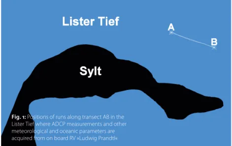
The study area of the Lister Tief is a tidal inlet of the German Bight in the North Sea bounded by the islands of Sylt to the south and Rømø to the north.
The positions of analysed runs along transect AB in the Lister Tief are presented in Fig. 1. Tide gauge station List is located 4.8 km southerly of transect AB. The seabed morphology in the Lister Tief is a complex configuration of continuously changing different bed forms. The submerged compound sand waves investigated in this study are four-di- mensional in space and time. Small-scale as well as megaripples are superimposed on sand waves as
1 Introduction
It is well known that a strong coherence exists between fluctuations of turbidity, phytoplancton, and suspended sediment concentration (SSC) induced by disturbances of tidal current veloci- ties. Substantial phenomena of SSC during two tidal cycles at two anchor stations in the southern North Sea were described by Joseph (1954). There he showed that a phase shift of 30 to 45 minutes happened between turbidity and current velocity maximum.
In situ observations in the past showed that sub- merged sand waves and internal waves associated with vertical current components can be sources of enhanced SSC in the water column above sea bottom topography. Often, such SSC features can come up to the water surface in shallow tidal seas of the ocean. The study presented by Hennings et al. (2002) showed that in a stratified two water An article by INGO HENNINGS and DAGMAr HErBErS
Ocean colour and its transparency are related to turbidity caused by substances in water like organic and inorganic material. One of the essential climate variables (ECV) is ocean colour. However, this implies the correct interpretation of observed water quality parameters. Acoustic Doppler Current Profiler (ADCP) data of the three-dimen- sional current-field, echo intensity, modulation of suspended sediment concentration (SSC), and related water levels and wind velocities have been analysed as a function of water depth above
submerged asymmetric compound sand waves during a tidal cycle in the Lister Tief of the German Bight in the North Sea.
Comparison and characteristics of
oceanographic in situ measurements and simulations above submerged sand waves in a tidal inlet
ADCP | SSC – suspended sediment concentration | TSM – total suspended sediment | asymmetric compound sand wave | dynamic buoyancy density | action density
Fig. 1: Positions of runs along transect AB in the Lister Tief where ADCP measurements and other meteorological and oceanic parameters are acquired from on board RV »Ludwig Prandtl«
Authors
Dr. Ingo Hennings and Dagmar Herbers are Research Scientists at the Geomar Helmholtz Centre for Ocean Research Kiel, Germany.
ihennings@geomar.de dherbers@geomar.de
presented here and already discussed in Van Dijk and Kleinhans (2005) as well as in Hennings and Herbers (2006). Analysed flood dominated sand waves have stoss slopes of the order of 2° and lee slopes up to 31°.
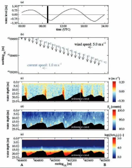
Water levels measured at tide gauge station List, wind and current velocities, vertical current com- ponents w , echo intensities e3 of fore beam No. 3 measured by ADCP and calculated SSC modula- tions expressed as log((δc / c0)3) of beam No. 3 as a function of water depth are presented. The con- stant SSC equilibrium term is defined by c0 and δc is the time-dependent perturbation term of the local SSC c. All parameters are measured and cal- culated over submerged asymmetric compound sand waves on the sea bottom during several runs along transect AB.
As an example, measurements during run 51 are shown in Fig. 2 for ebb tidal current phase. The du- ration of the measurement time is indicated by a vertical black line in Fig. 2a. Each run has been ro- tated by an angle of 19° in order to direct the cur- rent component u perpendicular to the sand wave crest. Hence, the v-component of the current field is minimised and can be neglected as a first ap- proximation. The rotation point is marked at the highest sand wave crest along the profile named as reference crest, shown in Fig. 2c to 2e. The cur- rent vectors shown in Fig. 2b are water depth averaged velocity values. Time interval of both, wind and current velocity arrows, is 30 s. Especially Fig. 2d illustrates the resuspension expressed by e3 in progress at ebb tides.
2.1 Time dependent measurements of vertical water depth averaged data
The base of Fig. 3 is a data set measured on 10 Au- gust 2002 between 0516 UTC and 0740 UTC while the research vessel was sailing against the ebb tid- al current direction over asymmetric flood orien- tated submerged sand waves along transect AB.
Fig. 3a shows the water level recorded at the tide gauge station List as a function of time. Herein, the acquisition times of five analysed single runs are marked. In Fig. 3b wind speeds are represented by arrows in a geocoded coordinate system. All other data are shown as a function of time and position in east-west direction. Fig. 3c to 3f illus- trate time series of vertically averaged values for current component u (east direction, indicated by a compass symbol with a red stick in Fig. 3c), echo intensity e3 of fore beam No. 3 measured by ADCP, vertical current component w, and calculated SSC modulations expressed as log((δc / c0)3) of beam No. 3. The water depth profiles of the asymmetric sand waves are shown in Fig. 3g to 3h.
Wind speeds between 5.8 m s–1 and 7.5 m s–1 from northerly directions were measured (Fig. 3b).
Negative, enhanced and positive values of u, e3, and w, respectively, show phase relationships with sand wave crests of the sea bed. In contrast, en- hanced log((δc / c0)3) shows a phase relationship
with the sand wave troughs of the sea bed. The parameters u, w, and log((δc / c0)3) are only weak- ly time dependent. All signatures of u, e3, w, and log((δc / c0)3), respectively, show spatially depend- ent variations in x-direction above the sand waves.
3 Theory of hydrodynamics above submerged sand waves
The focus of this section is the understanding and mathematical description of dynamic buoyancy density, total energy density, and action density above submerged asymmetric sand waves due to semi-diurnal lunar M2 tidal motion. The dynamic buoyancy density Ad is defined by
Ad = A~
d
≈ 1
· ρ · (ca – 1) · u–2 (1) F · zb 2
where ~A
d is the dynamic buoyancy in the water column of volume v(x,y,z) with the horizontal and
Fig. 2: Analysed data of ADCP of fore beam No. 3 as a function of position and water depth above asymmetric sand waves of run 51 along transect AB during ebb tidal phase between 0721 UTC and 0740 UTC on 10 August 2002; a) time series of water levels measured at the tide gauge station List; b) wind and current velocities, the two horizontal arrow-scales indicate a wind speed of 5.0 m s–1 and a current speed of 1.0 m s–1, respectively; along-track presentations of c) vertical current component w of the three-dimensional current field;
d) echo intensity e3; and e) calculated SSC modulation log((δc / c0)3). The timing of the measurement is marked by a vertical black line in a). The position of the reference crest is indicated at the highest sand wave crest of the run
(1), whereas Dätwyler (1934) normalised ca by 1.
The reason is here that both upwelling (positive) as well as downwelling (negative) values of ca can arise above sand waves. As a first approximation, for the downforce at the lee side of the sand wave, the negative value (downforce coefficient) of the lift coefficient ca is used here. Kinematic molecular viscosity and roughness effects at the sea bed are neglected.
The gradient of the dynamic buoyancy density perpendicular to the sand wave crest is derived as
∂Ad≈ (ca – 1) · ρ · u– ∂u–
(4)
∂x ∂x
Total energy density e is the sum of the potential energy density ep and the kinetic energy density ek. e = ep + ek = ρ · g (zR – 1 zb) + Ad (5) 2 (ca – 1)
where g is the acceleration due to gravity and zR
is the reference water depth at the trough of sand wave.
The action density N is defined by
N = ω' e (6)
where ω' is the radial frequency of the semi-diur- nal lunar M2 tidal wave with
ω' = 2π (7)
t
where t is the period of the semi-diurnal lunar M2 tidal wave.
Using equations (4) to (6), the gradient of the action density N perpendicular to the sand wave crest is derived as
∂N = ρ (– 1
g ∂zb + u– ∂u–
) (8)
∂x ω' 2 ∂x ∂x
Equation (8) shows that the gradient of the ac- tion density caused by the semi-diurnal M2 tidal wave is anti-proportional to the slope of the sea bed ∂zb / ∂x and proportional to the product of the vertical averaged current speed and its gradi- ent u– · (∂u– / ∂x), respectively.
Assuming that the vertical averaged current speed u– perpendicular to the sand wave crest obeys the continuity equation
u– · zb = const = c (9) and inserting equation (9) into equation (8) for
∂u– / ∂x, the following expression is derived
∂N = – ρ
∂zb( g + u–2
) (10)
∂x ω’ ∂x 2 zb
where ∂N / ∂x is proportional to u–2 and (zb)–1. vertical space coordinates x, y, and z, zb is the lo-
cal water depth, F is the infinitely thin horizontal plane element, ρ is the water density, ca is the di- mensionless lift coefficient, and u– is the vertical av- erage current velocity perpendicular to the sand wave crest. The dimensionless lift coefficient ca is defined by Dätwyler (1934) for a flat plate as
ca = π ( β
)1–2β (2)
sin(π · β) 1 – β and
β = α (3)
π
with α the slope angle of the stoss or lee plane of the sand wave. Both, stoss as well as lee sides of the sand wave were approximated by a flat plate.
However, here ca was subtracted by 1 in equation
Fig. 3: a) Time series of water level measured at tide gauge station List with acquisition times marked by No. 0 to 4 of 5 selected runs analysed during ebb tidal current phase from B to A while the research vessel is sailing against the current direction on 10 August 2002; b) measured wind velocities; the horizontal arrow-scale indicates a wind speed of 5.0 m s–1; c) time series of measured current component u; the east direction is marked by a red stick within the compass symbol; d) time series of echo intensity e3 of fore beam No. 3 measured by the ADCP; e) time series of measured vertical current component w; f) time series of calculated SSC modulation expressed as log((δc / c0)3). of beam No. 3; and g) – h) measured water depth profile of asymmetric submerged sand waves on the sea bed along transect AB
4 Evaluation and results of simulations
For all simulations a sand wave length L = 220 m and a sand wave height hc = 6 m are selected.
These parameters are typical values measured in the southern part of Lister Tief (see section 2). Sim- ulations of the sand wave profile with water depth zb, slope of the sea bed ∂zb / ∂x, vertical averaged tidal current speed u– and its gradient ∂u– / ∂x, re- spectively, dynamic buoyancy density Ad, gradient of the dynamic buoyancy density ∂Ad / ∂x, kinetic energy density ek, potential energy density ep, ac- tion density N, and gradient of the action density
∂N / ∂x as a function of space variable x are shown in Fig. 4a to 4e for ebb tidal current phase of asym- metric flood orientated sand waves. Typical values for the spatial resolutions Δx = 10 m and Δy = 1 m, zR = 25 m, gentle slope of sand wave αg = 2°, steep slope of sand wave αs = 9°, ρ = 1020 kg m–3, u– = 0.7 m s–1 at x with zb = zR, u– = 0.95 m s–1 at x = 0 m (sand wave crest), g = 9.82 m s–2, and t = 12.42 hours are calculated or inserted by using equations (1) to (10).
The sea bed profile with water depth zb which defines the asymmetric sand wave in black and the slope of the sea bed ∂zb / ∂x in red are shown in Fig. 4a.
The tidal current velocity u = u– is presented in black in Fig. 4b during ebb tidal current phase.
Due to the continuity equation (9) u– acquires its maximum absolute value at the sand wave crest.
The gradient of the tidal current speed ∂u / ∂x =
∂u– / ∂x is shown in red in Fig. 4b. A relative strong divergence flow ∂u– / ∂x = 0.007 s–1 is calculated at the steep slope of the sea bed.
The dynamic buoyancy density Ad, shown in black in Fig. 4c, strongly depends on the slope of the sea bed; a maximum negative value Ad = –50 N (downwelling) is calculated at the gentle slope of the sea bed and a maximum posi- tive value Ad = 160 N (upwelling) is calculated at the steep slope of the sea bed during ebb tidal current phase. A reversal of Ad is obtained dur- ing flood tidal current phase. These simulations agree with ADCP measurements of vertical posi- tive and negative components w of the tidal cur- rent velocity shown in Fig. 2c. The gradient of the dynamic buoyancy density ∂Ad / ∂x presented in Fig. 4c in red show low and high negative val- ues at both the gentle as well as the steep slope of the sea bed during ebb tidal current phase.
Again, a reversal of ∂Ad / ∂x took place during flood tidal current phase. Maximum values of
∂Ad / ∂x = –2.6 N m–1 are associated with maxi-
References
Dätwyler, Gottfried (1934): Untersu- chungen über das Verhalten von Tragflügelprofilen sehr nahe am Boden;
Diss.-Druckerei A.-G. Gebr. Leemann &
Co., Zürich, 110 p.
Hennings, Ingo; Margitta Metzner; G.-P.
de Loor (2002): The influence of quasi resonant internal waves on the radar imaging mechanism of shallow sea bottom topography; Oceanologica Acta, 25, pp. 87–99
Hennings, Ingo; Dagmar Herbers (2006):
Radar imaging mechanism of marine sand waves of very low grazing angle illumination caused by unique hydrodynamic interactions; Journal of Geophysical Research, 111 C1008, 15 p.
Hennings, Ingo; Dagmar Herbers (2014):
Suspended sediment signatures induced by shallow water undulating bottom topography; Remote Sensing of Environment, 140, pp. 294–305 Joseph, J. (1954): Die Sinkstofführung von
Gezeitenströmen als Austausch- problem; Archiv für Meteorologie, Geophysik und Bioklimatologie, Serie A 7, pp. 482–501 …
ments of e3 shown in Fig. 2d. The gradient of the action density ∂N / ∂x coloured in red in Fig. 4e is positive at the gentle slope and negative at the steep slope of the sand wave during ebb as well as flood tidal current phases. Maximum values of
∂N / ∂x = –6.0 · 106 N s m–3 are related to maxi- mum and high values of ∂zb / ∂x, ∂u / ∂x = ∂u– / ∂x, and ∂Ad / ∂x, respectively.
5 Conclusions
Based on in situ measurements of several oceano- graphic and meteorological parameters acquired in the Lister Tief, theory and simulations regarding the hydrodynamics above submerged asymmetric sand waves the following conclusions are drawn:
• Sand suspensions strongly depend on wave activity for high concentrations in the water column. Wave orbital motions close to the sea bed are induced by measured wind speeds between 11.7 m s–1 and 13.3 m s–1 from southeasterly direction to stir up sand particles.
• Bursts of w and e3 may be triggered at disturbances like megaripples superimposed on sand waves by current wave interaction at high current and wind speeds observed of opposite directions and measured at high spatial resolution.
• During moderate wind speeds between 5.8 m s–1 and 7.5 m s–1 from northerly direc- tions, negative, enhanced and positive values of u, e3, and w, respectively, show a definite phase relationship with the crest and upper gentle slope regions of sand waves during ebb tidal current phase while the research vessel is sailing with or against the current direction. In contrast, enhanced log((δc / c0)3) shows a phase relationship with trough re- gions of sand waves during ebb tidal current phase.
• Intense ejections caused by tidal current ve- locity transport higher SSC near the bottom boundary layer at the sand waves superim- posed by megaripples towards the free water surface. Such hydrodynamic upwelling mech- anism above sand waves creates distinct SSC signatures in remote sensing data visible in air- and space-borne optical imagery.
• During well developing flood and ebb tidal currents the intensities of u, w, and log((δc / c0)3) are only weakly time depend- ent. In contrast, e3 shows time dependence.
• The ADCP in situ measurements are to be consistent with simulations based on the ap- plied theory.
• The action density N and its gradient ∂N / ∂x due to semi-diurnal tide motion are the most important hydrodynamic parameters, which characterise comprehensively the dynam- ics of suspended sediment concentration (SSC) above submerged asymmetric sand waves. “
mum values of ∂u / ∂x = ∂u– / ∂x as it is also ex- pressed by equation (4).
The potential energy density ep shown in red and the kinetic energy density ek presented in black in Fig. 4d, respectively, are always positive and have same magnitudes during ebb as well as flood tidal current phases. However, the poten- tial energy density ep is a factor of about 349 to 500 J m–3 stronger than the kinetic energy density ek. Maximum values of ep and ek are corresponding with the sand wave crest where the current speed maximises.
The action density N shown in Fig. 4e as a black curve, is always positive and has the same mag- nitudes during ebb as well as flood tidal current phases with maximum N = 1.13 · 109 J s m–3 at the sand wave crest. The total action density N in the water column presented in Fig. 4e is higher at the spatial longer gentle slope region than at the shorter steep slope region of sand waves. There- fore, more suspended sediment particles are mov- ing upwards which is also shown by the measure-
Fig. 4: Simulations of oceanographic parameters applying equations (1) to (10) for ebb tidal current phase (current is directed from right to left) as a function of space variable x ; a) sand wave profile with water depth zb in black and slope of the sea bed ∂zb / ∂x in red, b) tidal current velocity u = u– in black and gradient of the tidal current velocity ∂u / ∂x
= ∂u– / ∂x in red, c) dynamic buoyancy density Ad in black and gradient of the dynamic buoyancy density ∂Ad / ∂x in red, d) kinetic energy density ek in black and potential energy density ep in red, and e) action density N in black and gradient of the action density ∂N / ∂x in red
…
Kwoll, Eva; Marius Becker; Christian Winter (2014): With or against the tide: The influence of bed form asymmetry on the formation of macroturbulence and suspended sediment patterns; Water Resources Research, 50, pp. 7800–7815 Tao, Zui; Ziwei Li; Bangyong Qin (2011):
Ocean sand ridges in the Yellow Sea observed by satellite remote sensing measurements; Remote Sensing, Environment and Transportation Engineering, International Conference, 24–26 June 2011, Nanjing, China;
Institute of Electrical and Electronics Engineers (IEEE), pp. 528–531 Van Dijk, Thaiënne A. G. P., Maarten G.
Kleinhans (2005): Processes controlling the dynamics of compound sand waves in the North Sea, Netherlands;
Journal of Geophysical Research, 110 F04S10, 15 p.