Comparison and Characteristics of Oceanographic In Situ Measurements and Simulations
above Submerged Sand Waves in a Tidal Inlet
Ingo HENNINGS and Dagmar HERBERS
Key words: Acoustic Doppler Current Profiler, suspended sediment concentration, asymmetric compound sand wave, dynamic buoyancy density, action density
SUMMARY
Ocean color and its transparency are related to turbidity caused by substances in water like organic and inorganic material. One of the essential climate variables (ECV) is ocean color.
However, this implies the correct interpretation of observed water quality parameters.
Acoustic Doppler Current Profiler (ADCP) data of the three-dimensional current-field, echo intensity, modulation of suspended sediment concentration (SSC), and related water levels and wind velocities have been analyzed as a function of water depth above submerged asymmetric compound sand waves during a tidal cycle in the Lister Tief of the German Bight in the North Sea. Signatures of vertical current component, echo intensities and calculated SSC modulations in the water column depend strongly on wind and current velocity. Bursts of vertical current component and echo intensity are triggered by sand waves itself as well as by superimposed megaripples due to current wave interaction at high current 1.0 m s-1 and wind speeds 10.0 m s-1, preferably of opposite directions, measured at high spatial resolution. The magnitude of currents and SSC modulations during ebb and flood tidal current phases are only weakly time dependent, whereas the local magnitudes of these parameters are variable in space above the sand waves. Intense ejections caused by tidal current velocity transport higher SSC near the bottom boundary layer at the sand waves superimposed by megaripples towards the free water surface. Such typical upwelling mechanism above sand waves creates distinct SSC signatures of remote sensing data visible in air- and space-borne optical imagery. Hydrodynamic parameters such as dynamic buoyancy density, total energy density and action density due to semi-diurnal M2 tide motion which are associated with sand waves are investigated and analyzed. Results and characteristics of simulated hydrodynamic parameters in coastal waters above sand waves are presented. It is shown that ADCP measurements are to be consistent with simulations based on the applied theory.
1. INTRODUCTION
It is well known that a strong coherence exists between fluctuations of turbidity, phytoplankton, and suspended sediment concentration (SSC) induced by disturbances of tidal current velocities. Substantial phenomena of SSC during two tidal cycles at two anchor
stations in the southern North Sea were described by Joseph (1954). There he showed that a phase shift of 30-45 minutes happened between turbidity and current velocity maximum.
In situ observations in the past showed that submerged sand waves and internal waves associated with vertical current components can be sources of enhanced SSC in the water column above sea bottom topography. Often, such SSC features can come up to the water surface in shallow tidal seas of the ocean. The study presented by Hennings et al. (2002) showed that in a stratified two water layer system, simultaneous reductions in the near-surface water temperature and beam transmittance have been recorded, whereas fluorescence data are increased above sand waves. A good linear relationship between water depth and total suspended sediment (TSM) data derived from Moderate Resolution Imaging Spectroradiometer (MODIS) measurements above sand ridges in the southern Yellow Sea was found by Tao et al. (2011). The TSM concentration was proportional to the inverse water depth; high TSM concentrations were located above shallow parts of sand ridges. It was shown by Hennings and Herbers (2014) that strong currents flowing over steep bottom topography are able to stir up the sediments to form both a general continuum of SSC and localized pulses of higher SSC in the vicinity of the causative bed feature itself. Tide- dependent variations in the formation and dynamics of suspended sediment patterns coupled to mean flow and turbulence above asymmetric bedforms were examined by Kwoll et al.
(2014).
2. MEASUREMENTS CONDUCTED DURING A TIDAL CYCLE
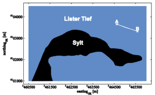
The study area of the Lister Tief is a tidal inlet of the German Bight in the North Sea bounded by the islands of Sylt to the South and Rømø to the North. The positions of analyzed runs along transect AB in the Lister Tief are presented in Figure 1. Tide gauge station List is located 4.8 km southerly of transect AB. The seabed morphology in the Lister Tief is a complex configuration of continuously changing different bed forms. The submerged compound sand waves investigated in this study are four-dimensional in space and time.
Small-scale as well as megaripples are superimposed on sand waves as presented here and already discussed in Van Dijk and Kleinhans (2005) as well as in Hennings and Herbers (2006). Analyzed flood dominated sand waves have stoss slopes of the order of 2° and lee slopes up to 31°.
Figure 1: Positions of runs along transect AB in the Lister Tief where ADCP measurements and other meteorological and oceanic parameters are acquired from on board R/V Ludwig Prandtl.
Figure 2: Analyzed data of ADCP of fore beam No. 3 as a function of position and water depth above asymmetric sand waves of run 51 along transect AB indicated in Fig. 1 during ebb tidal phase at 0721-0740 UTC on 10 August 2002; a) time series of water levels measured at the tide gauge station List, b) wind and current velocities, the two horizontal arrow-scales indicate a wind speed of 5.0 m s-1 and a current speed of 1.0 m s-1, respectively; along-track presentations of c) vertical current component w of the three-dimensional current field, d) echo intensity E3, and e) calculated SSC modulation
/ 0 3
log c c . The timing of the measurement is marked by a vertical black line in a).
The position of the reference crest is indicated at the highest sand wave crest of the run.
Water levels measured at tide gauge station List, wind and current velocities, vertical current components w, echo intensities E3 of fore beam No. 3 measured by ADCP and calculated SSC modulations expressed as log
c/c0
3
of beam No. 3 as a function of water depth are
presented. The constant SSC equilibrium term is defined by c0 and c is the time-dependent
perturbation term of the local SSC c. All parameters are measured and calculated over
submerged asymmetric compound sand waves on the sea bottom during several runs along
transect AB.
As an example, measurements during run 51 are shown in Figures 2a-e for ebb tidal current phase. The duration of the measurement time is indicated by a vertical black line in Fig. 2a.
Each run has been rotated by an angle of 19° in order to direct the current component u perpendicular to the sand wave crest. Hence, the v-component of the current field is minimized and can be neglected as a first approximation. The rotation point is marked at the highest sand wave crest along the profile named as reference crest, shown in Figs. 2c-e. The current vectors shown in Fig. 2b are water depth averaged velocity values. Time interval of both, wind and current velocity arrows, is 30 s. Especially Fig. 2d illustrates the resuspension expressed by E3 in progress at ebb tides.
2.1. Time dependent measurements of vertical water depth averaged data
The base of Figure 3 is a dataset measured on 10 August 2002 between 0516 UTC and 0740 UTC while the research vessel was sailing against the ebb tidal current direction over asymmetric flood orientated submerged sand waves along transect AB. Fig. 3a shows the water level recorded at the tide gauge station List as a function of time. Herein the acquisition times of five analyzed single runs are marked. In Fig. 3b wind speeds are represented by arrows in a geocoded coordinate system. All other data are shown as a function of time and position in east-west direction. Figs. 3c-f illustrate time series of vertically averaged values for current component u (east direction, indicated by a compass symbol with a red stick in Fig. 3c), echo intensity E3 of fore beam No. 3 measured by ADCP, vertical current component w, and calculated SSC modulations expressed as log
c/c0
3
of beam No. 3.
The water depth profiles of the asymmetric sand waves are shown in Figs. 3g-h.
Wind speeds between 5.8 m s-1 and 7.5 m s-1 from northerly directions were measured (Fig.
3b). Negative, enhanced and positive values of u, E3, and w, respectively, show phase relationships with sand wave crests of the sea bed. In contrast, enhanced log
c/c0
3
shows
a phase relationship with the sand wave troughs of the sea bed. The parameters u, w, and
/ 0 3
log c c are only weakly time dependent. All signatures of u, E3, w, and
/ 0 3
log c c , respectively, show spatially dependent variations in x-direction above the sand waves.
Figure 3: a) Time series of water level measured at tide gauge station List with acquisition times marked by Nos. 0-4 of 5 selected runs analyzed during ebb tidal current phase from B to A while the research vessel is sailing against the current direction on 10 August 2002, b) measured wind velocities; the horizontal arrow-scale indicates a wind speed of 5.0 m s-1, c) time series of measured current component u; the east direction is marked by a red stick within the compass symbol, d) time series of echo intensity E3 of fore beam No. 3 measured by the ADCP, e) time series of measured vertical current component w, f) time series of calculated SSC modulation expressed as
/ 0 3
log c c of beam No. 3, and g) - h) measured water depth profile of asymmetric submerged sand waves on the sea bed along transect AB (for location see Fig. 1).
3. THEORY OF HYDRODYNAMICS ABOVE SUBMERGED SAND WAVES
The focus of this section is the understanding and mathematical description of dynamic buoyancy density, total energy density, and action density above submerged asymmetric sand waves due to semi-diurnal lunar M2 tidal motion. The dynamic buoyancy density Ad is defined by
1
22
~ 1
u z c
F
A A a
b d
d
(1)
where A~d
is the dynamic buoyancy in the water column of volume V
x,y,z
with the horizontal and vertical space coordinates x, y, and z, zb is the local water depth, F is the infinitely thin horizontal plane element, is the water density, ca is the dimensionless lift coefficient, and u is the vertical average current velocity perpendicular to the sand wave crest. The dimensionless lift coefficient ca is defined by Dätwyler (1934) for a flat plate as
1 2
1 sin
ca (2)
and
(3)
with the slope angle of the stoss or lee plane of the sand wave. Both, stoss as well as lee sides of the sand wave were approximated by a flat plate. However, here ca was subtracted by 1 in equation (1), whereas Dätwyler (1934) normalized ca by 1. The reason is here that both upwelling (positive) as well as downwelling (negative) values of ca can arise above sand waves. As a first approximation, for the downforce at the lee side of the sand wave, the negative value (downforce coefficient) of the lift coefficient ca is used here. Kinematic molecular viscosity and roughness effects at the sea bed are neglected.
The gradient of the dynamic buoyancy density perpendicular to the sand wave crest is derived as
x u u x c
A
a d
1 (4)
Total energy density E is the sum of the potential energy density Ep and the kinetic energy density Ek
1
2 1
a d b
R k
p c
z A z
g E
E
E (5)
where g is the acceleration due to gravity and zR is the reference water depth at the trough of sand wave.
The action density N is defined by
'
N E (6)
where ' is the radial frequency of the semi-diurnal lunar M2 tidal wave with
T
' 2 (7)
where T is the period of the semi-diurnal lunar M2 tidal wave.
Using equations (4) – (6), the gradient of the action density N perpendicular to the sand wave crest is derived as
x u u x g z x
N b
2 1
'
(8)
Equation (8) shows that the gradient of the action density caused by the semi-diurnal M2 tidal wave is anti-proportional to the slope of the sea bed zb /x and proportional to the product of the vertical averaged current speed and its gradient u
u/x
, respectively.Assuming that the vertical averaged current speed u perpendicular to the sand wave crest obeys the continuity equation
c const z
u b (9) and inserting equation (9) into equation (8) for u/x, the following expression is derived
b b
z u g x z x
N 2
' 2
(10)
where N/x is proportional to u2 and
zb 1.4. EVALUATION AND RESULTS OF SIMULATIONS
For all simulations a sand wave length L = 220 m and a sand wave height hc = 6 m are selected. These parameters are typical values measured in the southern part of Lister Tief (see section 2). Simulations of the sand wave profile with water depth zb, slope of the sea bed
x zb
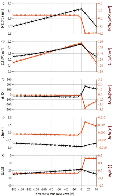
/ , vertical averaged tidal current speed u and its gradient u/x, respectively, dynamic buoyancy density Ad, gradient of the dynamic buoyancy density Ad /x, kinetic energy density Ek, potential energy density Ep, action density N, and gradient of the action density N/x as a function of space variable x are shown in Figs. 4a-e for ebb tidal current phase of asymmetric flood orientated sand waves. Typical values for the spatial resolutions
x = 10 m and y = 1 m, zR = 25 m, gentle slope of sand wave g = 2°, steep slope of sand wave s = 9°, = 1020 kg m-3, u = 0.7 m s-1 at x with zb = zR, u = 0.95 m s-1 at x = 0 m (sand wave crest), g = 9.82 m s-2, and T = 12.42 hours are calculated or inserted by using equations (1) - (10).
The sea bed profile with water depth zb which defines the asymmetric sand wave in black and the slope of the sea bed zb /x in red are shown in Fig. 4a.
The tidal current velocity uu is presented in black in Fig. 4b during ebb tidal current phase. Due to the continuity equation (9) u acquires its maximum absolute value at the sand wave crest. The gradient of the tidal current speed u/xu/x is shown in red in Fig. 4b.
A relative strong divergence flow u/x = 0.007 s-1 is calculated at the steep slope of the sea bed.
The dynamic buoyancy density Ad, shown in black in Fig. 4c, strongly depends on the slope of the sea bed; a maximum negative value Ad = -50 N (downwelling) is calculated at the gentle slope of the sea bed and a maximum positive value Ad = 160 N (upwelling) is calculated at the steep slope of the sea bed during ebb tidal current phase. A reversal of Ad is obtained during flood tidal current phase. These simulations agree with ADCP measurements of vertical positive and negative components w of the tidal current velocity shown in Fig. 2c.
The gradient of the dynamic buoyancy density Ad /x presented in Fig. 4c in red show low and high negative values at both the gentle as well as the steep slope of the sea bed during ebb tidal current phase. Again, a reversal of Ad /x took place during flood tidal current phase.
Maximum values of Ad /x = -2.6 N m-1 are associated with maximum values of x
u x
u
/ / as it is also expressed by equation (4).
The potential energy density Ep shown in red and the kinetic energy density Ek presented in black in Fig. 4d, respectively, are always positive and have same magnitudes during ebb as well as flood tidal current phases. However, the potential energy density Ep is a factor of about 349-500 J m-3 stronger than the kinetic energy density Ek. Maximum values of Ep and
Ek are corresponding with the sand wave crest where the current speed maximizes.
The action density N shown in Fig. 4e as a black curve, is always positive and has the same magnitudes during ebb as well as flood tidal current phases with maximum N = 1.13.109 J s m-3 at the sand wave crest. The total action density N in the water column presented in Fig.
4e is higher at the spatial longer gentle slope region than at the shorter steep slope region of sand waves. Therefore, more suspended sediment particles are moving upwards which is also shown by the measurements of E3 shown in Fig. 2d. The gradient of the action density
x N
/ colored in red in Fig. 4e is positive at the gentle slope and negative at the steep slope of the sand wave during ebb as well as flood tidal current phases. Maximum values of N/x
= -6.0.106 N s m-3 are related to maximum and high values of zb /x, u/xu/x, and x
Ad
/ , respectively.
Figure 4: Simulations of oceanographic parameters applying equations (1)-(10) for ebb tidal current phase (current is directed from right to left) as a function of space variable x; a) sand wave profile with water depth zb in black and slope of the sea bed zb /x in red, b) tidal current velocity uu in black and gradient of the tidal current velocity
x u x
u
/ / in red, c) dynamic buoyancy density Ad in black and gradient of the dynamic buoyancy density Ad /x in red, d) kinetic energy density Ek in black and potential energy density Ep in red, and e) action density N in black and gradient of the action density N/x in red.
5. CONCLUSIONS
Based on in situ measurements of several oceanographic and meteorological parameters acquired in the Lister Tief, theory and simulations regarding the hydrodynamics above submerged asymmetric sand waves the following conclusions are drawn:
1. Sand suspensions strongly depend on wave activity for high concentrations in the water column. Wave orbital motions close to the sea bed are induced by measured wind speeds between 11.7 m s-1 and 13.3 m s-1 from southeasterly direction to stir up sand particles.
2. Bursts of w and E3 may be triggered at disturbances like megaripples superimposed on sand waves by current wave interaction at high current and wind speeds observed of opposite directions and measured at high spatial resolution.
3. During moderate wind speeds between 5.8 m s-1 and 7.5 m s-1 from northerly directions, negative, enhanced and positive values of u, E3, and w, respectively, show a definite phase relationship with the crest and upper gentle slope regions of sand waves during ebb tidal current phase while the research vessel is sailing with or against the current direction. In contrast, enhanced log
c/c0
3
shows a phase relationship with trough regions of sand
waves during ebb tidal current phase.
4. Intense ejections caused by tidal current velocity transport higher SSC near the bottom boundary layer at the sand waves superimposed by megaripples towards the free water surface. Such hydrodynamic upwelling mechanism above sand waves creates distinct SSC signatures in remote sensing data visible in air- and space-borne optical imagery.
5. During well developing flood and ebb tidal currents the intensities of u, w, and
/ 0 3
log c c are only weakly time dependent. In contrast, E3 shows time dependence.
6. The ADCP in situ measurements are to be consistent with simulations based on the applied theory.
7. The action density N and its gradient N/x due to semi-diurnal tide motion are the most important hydrodynamic parameters which characterize comprehensively the dynamics of suspended sediment concentration (SSC) above submerged asymmetric sand waves.
REFERENCES
Dätwyler, G.: Untersuchungen über das Verhalten von Tragflügelprofilen sehr nahe am Boden.
Promotionsarbeit, Diss.-Druckerei A.-G. Gebr. Leemann & Co., Zürich, Schweiz, pp. 110, 1934.
Hennings, I., Metzner, M., de Loor, G.-P.: The influence of quasi resonant internal waves on the radar imaging mechanism of shallow sea bottom topography. Oceanologica Acta, 25, p. 87-99, 2002.
Hennings, I., Herbers, D.: Radar imaging mechanism of marine sand waves of very low grazing angle illumination caused by unique hydrodynamic interactions. Journal of Geophysical Research, 111 C1008, pp. 15, 2006. doi:10.1029/2005JC003302
Hennings, I., Herbers, D.: Suspended sediment signatures induced by shallow water undulating bottom topography. Remote Sensing of Environment, 140, p. 294-305, 2014. doi:10.1016/j.rse.2013.09.004 Joseph, J.: Die Sinkstofführung von Gezeitenströmen als Austauschproblem. Archiv für Meteorologie, Geophysik und Bioklimatologie, Serie A 7, p. 482-501, 1954. doi: 10.1007/BF02277938
Kwoll, E., Becker, M., Winter, C.: With or against the tide: The influemce of bed form asymmetry on the formation of macroturbulence and suspended sediment patterns. Water Resources Research, 50, p.
7800-7815, 2014. doi:10.1002/2013WR014292
Tao, Z., Li, Z.-W., Qin, B.J.: Ocean sand ridges in the Yellow Sea observed by satellite remote sensing measurements. Remote Sensing, Environment and Transportation Engineering, International Conference, Proceedings of a meeting held 24-26 June 2011, Nanjing, China, Publisher: Institute of Electrical and Electronics Engineers (IEEE), p. 528-531, 2011.
Van Dijk, T.A.G.P., Kleinhans, M.G.: Processes controlling the dynamics of compound sand waves in the North Sea, Netherlands. Journal of Geophysical Research, 110 F04S10, pp. 15, 2005.
doi:10.1029/2004JF000173 BIOGRAPHICAL NOTES
Ingo Hennings was born in Veerssen (Uelzen), Germany, on 30 May 1952. From 1968 to 1978, he sailed on board of ocean-going merchant vessels and is holder of the German ship captain’s certificate foreign trade master (AG). He received the diploma degree in
oceanography from the University of Hamburg, Germany, in 1984, and the Ph.D. degree in physics/electrical engineering from the University of Bremen, Germany, in 1988. From 1985 to 1988, he worked in marine remote sensing at the GKSS Research Center (now: Helmholtz- Zentrum Geesthacht (HZG)) in Geesthacht, Germany. Since 1989, he has been a Research Scientist at the GEOMAR Helmholtz Centre for Ocean Research Kiel, Germany. His research interests include marine remote sensing with imaging radar and optical sensors as well as sea bottom topography current wave interaction.
CONTACTS
Dr. Ingo Hennings
GEOMAR Helmholtz Centre for Ocean Research Kiel Wischhofstrasse 1-3
D-24148 Kiel Germany
Tel. + (49)4316002312 Fax + (49)431600132312 Email: ihennings@geomar.de Web site: www.geomar.de