An invitation to solve global optimization problems by the use of geometric branch-and-bound methods
Daniel Scholz
daniel.scholz@mehr-davon.de
Manuscript (Version of March 25, 2014)
Abstract
Geometric branch-and-bound algorithms are well-known solution techniques in de- terministic global optimization. To keep the use of these solution methods as simple as possible, we suggest an easy-to-use JavaScript tool which includes the branch-and- bound algorithm and an interval arithmetic package. Hence, one only has to implement the objective function and the calculation of the lower bounds if one wants to solve a suitable continuous optimization problem. The present work provides an extensive doc- umentation on how to use the code as well as several example problems for instance from the field of location theory which were solved by the use of the JavaScript tool.
The suggested code as well as all examples given in this work can be downloaded from our homepage mentioned at the end of the introduction.
Keywords: deterministic global optimization, geometric branch-and-bound, location theory, continuous optimization, JavaScript tool.
1 Introduction
Indeterministic global optimization one wants to find the global minima of some real- valued functions. Many new theoretical and computational contributions to deterministic global optimization have been developed in the last decades andgeometric branch-and- bound methods arose to a commonly used solution technique, in particular if one deals with a few number of continuous variables.
The main task throughout all geometric branch-and-bound algorithms is to calculate lower bounds on the continuous objective function and several methods to do so can be found in the literature: Some general techniques can be found in Horst and Tuy (1996), Horst et al.
(2000), Hansen and Jaumard (1995), Horst and Thoai (1999), and Tuy and Horst (1988).
Constructing lower bounds by the use of interval analysis was discussed in Ratschek and Rokne (1988), Hansen (1992), and Ratschek and Voller (1991). Moreover, some particular algorithms for facility location problems were suggested in Hansen et al. (1985), Plas- tria (1992), Drezner and Suzuki (2004), Drezner (2007), Blanquero and Carrizosa (2009), Sch¨obel and Scholz (2010a), Tuy et al. (1995) and Tuy (1996). For a summary of all these bounding techniques we refer to Scholz (2012a).
Our main intension of the present work is an easy-to-use tool for the solution of global optimization problems by the use of geometric branch-and-bound methods. To this end, following Scholz (2012a), the algorithm was implemented in JavaScript in such a way that one basically only has to specify the objective function and a corresponding bounding operation. JavaScript was chosen since the code can be run on almost every modern browser without any further software, and, furthermore, the code can be edited with any text editor.
Hence, the suggested tool can be perfectly used for education purposes.
In the following Section 2 we start with basic notations and a brief summary of the geometric branch-and-bound algorithm. For theoretical results including a convergence theory and for the calculation of lower bounds we refer to Scholz (2012a). Moreover, the section includes a summary of interval analysis, i.e., a technique which provides some simple lower bounds.
The main contribution can be found in Section 3 where we give an extensive documentation of the suggested JavaScript tool including an description of the software architecture as well as two first example problems. Furthermore, the section includes a documentation of the interval arithmetic package as well as the problem visualization package which are also included in the JavaScript code. Next, the following Section 4 gives some example problems which can be solved efficiently using the suggested JavaScript geometric branch-and-bound tool. We remark that the JavaScript branch-and-bound tool as well as all examples given in the present work can be downloaded from:
www.mehr-davon.de/gbb/
2 Geometric branch-and-bound methods
Following Scholz (2012a), this section summarizes the geometric branch-and-bound proto- type algorithm which was implemented in a JavaScript tool as described in Section 3. After some basic notations, we present the general geometric branch-and-bound technique includ- ing some further remarks and comments. Finally, we briefly summarize interval arithmetics which might be used to obtain required bounds throughout the algorithm.
2.1 Notations
The following notations are similar to those suggested in Sch¨obel and Scholz (2010b) and Scholz (2012a).
Notation 1. A compactbox with sides parallel to the axes is denoted by X = [xL1, xR1] × . . . × [xLn, xRn] ⊂ Rn.
The diameter of a box X⊂Rnis δ(X) =
q
xR1 −xL12
+. . .+ (xRn −xLn)2 and thecenter of a boxX ⊂Rn is defined by
c(X) = 1
2(xL1 +xR1), . . . , 1
2(xLn+xRn)
.
In the following, we consider the minimization of a continuous function f :X→R,
where we assume a boxX⊂Rn as feasible area, i.e.,
X = [xL1, xR1] × . . . × [xLn, xRn] ⊂ Rn. Next, we define bounding operations as follows.
Notation 2. LetX ⊂Rn be a box and considerf :X →R. Abounding operation is a procedure to calculate for any subboxY ⊂X a lower bound LB(Y)∈Rwith
LB(Y) ≤ f(x) for all x∈Y and to specify a pointr(Y)∈Y.
Several general bounding operations are derived in Sch¨obel and Scholz (2010b) and Scholz (2012b) and summarized in Scholz (2012a). Moreover, note that the choice ofr(Y) is often only important for some theoretical result as discussed in the previously cited references.
If it is unclear how to specify r(Y), a general choice is the center ofY, that is, r(Y) = c(Y).
2.2 The algorithm
The general idea of all geometric branch-and-bound algorithms cited in Section 1 is the same: Subboxes of the feasible area are bounded from below making use of a bounding operation as defined before. If the bounds are not sharp enough, some boxes are split into smaller ones according to a given splitting rule. This procedure repeats until the algorithm finds an optimal solutionx∗∈X within an absolute accuracy of ε >0.
To sum up, for the following geometric branch-and-bound algorithm assume an objective functionf and a feasible boxX. Moreover, we need a bounding operation, a splitting rule, and an absolute accuracy of ε >0.
( 1 ) LetX be a list of boxes and initializeX :={X}.
( 2 ) Apply the bounding operation toX and setUB:=f(r(X)) andx∗ :=r(X).
( 3 ) IfX =∅, the algorithm stops. Else set
δmax := max{δ(Y) : Y ∈ X }.
( 4 ) Select a box Y ∈ X with δ(Y) = δmax and split it according to a selected splitting rule intoscongruent smaller subboxes Y1 toYs.
( 5 ) SetX = (X \Y)∪ {Y1, . . . , Ys}, i.e., deleteY fromX and addY1, . . . , Ys. ( 6 ) Apply the bounding operation toY1, . . . , Ys and set
UB = min{UB, f(r(Y1)), . . . , f(r(Ys))}.
IfUB=f(r(Yk)) for a k∈ {1, . . . , s}, set x∗ =r(Yk).
( 7 ) For allZ ∈ X, ifLB(Z) +ε≥UB set X =X \Z, i.e., deleteZ from X. ( 8 ) Return to Step( 3 ).
The selected box Y in Step ( 4 ) has to be split into ssubboxes Y1 toYs according to one of the following splitting rules:
( 1 ) For boxes in small dimensions, say n≤ 3, we suggest a split into s= 2n congruent subboxes.
( 2 ) In higher dimensions, boxes can be bisected perpendicular to the direction of the maximum width component in two subboxesY1 and Y2.
For some theoretical results regarding the termination of the algorithm, we refer to Sch¨obel and Scholz (2010b) and Scholz (2012a).
2.3 Interval arithmetic
The main task throughout any geometric branch-and-bound algorithm is the calculation of the required lower bounds. Interval arithmetic is a general framework for calculations with intervals, see, e.g., Ratschek and Rokne (1988) or Neumaier (1990), which is also a suitable tool for the calculation of lower bounds as outlined in the textbook Hansen (1992) or in Ratschek and Voller (1991).
Since the following JavaScript tool also includes an interval arithmetic package, this sub- section summarizes the basic ideas of interval arithmetic for the calculation of the required bounds as given in Scholz (2012b). Note that we assume compact intervals at all times throughout this paper.
Notation 3. A (compact) intervalX is denoted by X = [a, b] ⊂ R
with a≤ b. Moreover, the left and right endpoints are denoted by XL =a and XR = b, respectively.
Next, arithmetic operations between intervals are defined as follows.
Definition 4. LetX= [a, b] andY = [c, d] be two intervals. Then theinterval arithmetic is given by
X ? Y := {x ? y : x∈X, y∈Y},
where?denotes the addition, multiplication, subtraction, division, minimum, or maximum as long as x ? y is defined for all x, y∈Y.
By definition,X ? Y again yields an interval which containsx ? yfor allx∈X and y∈Y and which can be computed easily. Apart from interval arithmetic also interval operations are defined as follows.
Definition 5. LetX= [a, b] be an interval. Then the interval operation is given by op(X) := {op(x) : x∈X} =
minx∈Xop(x),max
x∈X op(x)
,
whereop:X →R denotes a continuous function such thatop(X) is an interval.
Definition 6. Aninterval function F(X1, . . . , Xn) is an interval valued function withn intervals as argument using interval arithmetics and interval operations as defined before.
Example 1. An interval function F(X, Y) with two intervals X and Y as argument is F(X, Y) =
X+Y Y2+ [1,1]
.
For example, we obtain
F([0,2],[−2,1]) =
[0,2] + [−2,1]
[−2,1]2+ [1,1]
=
[−2,3]
[1,5]
= [−2,3]
= [0,3].
Definition 7. Letf(x1, . . . , xn) be a fixed representation of a real-valued function withn real numbers as argument using arithmetics and operations such that the corresponding interval arithmetics and interval operations are defined.
Then the natural interval extension of f(x1, . . . , xn) is given by the interval function F(X1, . . . , Xn) where arithmetics and operations are replaced by their corresponding inter- val arithmetics and interval operations.
Example 2. The natural interval extension of
f(x, y) = 4·x2+ sin(y) x2+ 1 is given by
F(X, Y) = [4,4]·X2+ sin(Y) X2+ [1,1]
where X and Y are intervals.
The natural interval extension leads to general lower bounds as required throughout the geometric branch-and-bound algorithm. To this end, we need the following statement which can be found in any standard textbook of interval analysis such as Ratschek and Rokne (1988), Neumaier (1990), or Hansen (1992).
Theorem 1 (Fundamental theorem of interval analysis). LetF(X1, . . . , Xn)be the natural interval extension of f(x1, . . . , xn). Then
f(Y1, . . . , Yn) ⊆ F(Y1, . . . , Yn) for all intervals Yk⊆Xk for k= 1, . . . , n, where
f(Y1, . . . , Yn) := {f(x1, . . . , xn) : xk∈Yk fork= 1, . . . , n}.
Proof. See, for instance, Hansen (1992).
In other words, if we consider an optimization problem with a real-valued function f, then the natural interval extension F of f yields lower bounds as required throughout the geometric branch-and-bound algorithm, see Subsection 3.5.
On the other hand, we remark the bounds obtained from the natural interval extension might not be sharp enough to solve problems in a reasonable amount of time. For some more sophisticated bounding operations we refer to Scholz (2012b), Sch¨obel and Scholz (2010b), and Scholz (2012a).
3 Documentation of the JavaScript tool
The suggested geometric branch-and-bound method presented in Section 2 was implemented in JavaScript including an interval arithmetic package as well as a problem visual- ization package.
We remark that the biggest advantage of JavaScript is that it can be run on almost every modern internet browser without any further software. Moreover, the code for the problem formulation can be modified with any text editor. Hence, the JavaScript tool can be perfectly used for education purposes which was our main intension throughout this work.
On the other hand, a disadvantage is the run time. Since JavaScript is a scripting language, the code is not compiled and it needs to be interpreted at any time the code is running.
Therefore, some much more efficient implementations of the examples given in Section 4 are possible although the JavaScript tool yields adequate results for example for medium-sized facility location problems, see Section 4.
In this section, we first explain the use of the application in a web browser before explaining the software architecture of the proposed JavaScript code where we distinguish between mandatory and optional functions. Next, documentations of the interval arithmetic package
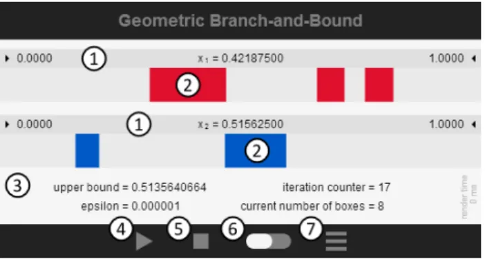
Figure 1. Control panel of the JavaScript branch-and-bound tool for an example problem withn= 2.
and the problem visualization package are given. The section ends with an detailed example problem making use of all the packages explained before.
3.1 The application
The JavaScript tool runs on every modern internet browser and provides a control panel including the elements as well as a visualization of the progress of the branch-and-bound algorithm as given in Figure 1:
( 1 ) For each variablex1 to xn, the bounds of the initial box as well as the current best- known solution are displayed.
( 2 ) The colored regions are subboxes which may contain the optimal solution. In other words, if some sub-intervals are not colored, they can not contain any optimal solution (up to the absolute accuracy ofε).
( 3 ) The output text shows the best-known upper bound, the pre-defined absolute accu- racyε, the number of iterations while running the algorithm, and the current number of boxes, i.e., the number of elements in X.
( 4 ) The first button is to start and pause the algorithm.
( 5 ) The second button stops and resets the algorithm. Note that the init problem function described below is called once the button is pressed.
( 6 ) This button is to change between a slow and a fast mode. In the slow mode, the algorithm performs two iterations every second. In the fast mode, the algorithm runs as fast as possible.
( 7 ) The last button deactivates the colored regions. This might be useful if the current number of boxes exceeds some limits which might leed to high rendering times.
3.2 Software architecture
Three files are needed if one wants to solve a minimization problem by the use of the JavaScript branch-and-bound tool, see Figure 2:
Figure 2. Software architecture of the proposed JavaScript tool.
( 1 ) index.html. This file includes the JavaScript source files and contains the canvas element which is needed to illustrate the progress of the branch-and-bound algorithm.
( 2 ) branch-and-bound.js. This file contains the source-code of the JavaScript branch- and-bound tool. The file can be downloaded from
www.mehr-davon.de/gbb/
and should not be edited at any time.
( 3 ) problem.js. This file contains the problem definition, i.e., the objective function as well as some mandatory and optional parameters and functions described below.
Mandatory items
There are some mandatory items which should always be used in the index.htmlfile, see Figure 2 and Figure 3(a):
( 1 ) Line 4 includes the branch-and-bound tool filebranch-and-bound.js.
( 2 ) Line 5 includes the problem definition fileproblem.js.
( 3 ) Theonloadstatement in line 8 ensures that the branch-and-bound commences at the time the html file is loaded.
( 4 ) Thecanvaselement with idcanvas B in line 9 is needed to illustrate the progress of the branch-and-bound algorithm and to show the control panel as given in Figure 1.
In addition, the branch-and-bound tool requires the following mandatory variables and functions in the problem.jsfile, see Figure 2 and Figure 3(b):
( 1 ) The variabledimension in line 1 defines the dimension of the problem which should be an integer value greater than or equal to one.
( 2 ) The variable X in line 2 defines the initial box X of the problem. In the one- dimensional case,Xis an interval defined by its endpoints. In the higher dimensional case,Xis an array of intervals.
(a)Source-code of theindex.htmlfile.
(b)Source-code of theproblem.jsfile.
Figure 3. One-dimensional example of the JavaScript tool: The objective functionf(x) = sin(x) is minimized over the intervalX= [0,8] with an absolute accuracy ofε= 10−6.
( 3 ) The variableepsilonin line 3 defines the absolute accuracy for the branch-and-bound algorithm.
( 4 ) The functionf in line 5 defines the objective function. Note that the argument xis an array starting with index 0 if the dimension is greater than one.
( 5 ) The function LB in line 9 specifies the lower bound for any box Y. In the one- dimensional case,Yis an interval defined by its endpoints. In the higher dimensional case,Yis an array of intervals.
Example 3. Figure 3 presents the source-code of the index.htmland the problem.js files for an example only using the mandatory items as summarized in Figure 2. Here, the one-dimensional objective function
f(x) = sin(x)
is minimized over the box or intervalX = [0,8]with an absolute accuracy of ε= 10−6. The lower bounds are calculated using the Lipschitzian bound operation as presented in Scholz (2012a) and references therein.
Theone-dimensional example problem is to minimize the function f(x) = sin(x)
over the box or interval X= [0,8].
Optional items
Apart from the mandatory items, the branch-and-bound tool offers some optional features.
In the index.htmlfile, there is only one optional item, see Figure 2:
( 1 ) The canvaselement with idcanvas P is needed to illustrate the problem which also requires the function plot problemas described in the following.
In the problem.jsfile, one may use the following options, see Figure 2:
( 1 ) The variable split option defines the splitting rule. If split option has a value of one, boxes are split into 2n congruent subboxes. Otherwise, boxes are bisected perpendicular to the direction of the maximum width component.
If there is no variable split option defined, the branch-and-bound tool uses the splitting rule as suggested in Subsection 2.2.
( 2 ) The functionrmay be used to define the specific pointr(Y) of the bounding operation, see Notation 2. Note that the function should return an array if the dimension is greater than one.
If there is no functionrdefined, the branch-and-bound tool uses of the center of Y. ( 3 ) The functioninit problemis called to initialize some problem instances before run-
ning the branch-and-bound algorithm, see Subsection 3.5.
( 4 ) Finally, the functionplot problemis needed to illustrate the problem, see Example 4 and Subsection 3.4.
Example 4. We want to extend Example 3 in such a way that the objective function is plotted using the problem visualization package described below.
To this end, theindex.htmlfile needs a secondcanvaselement with idcanvas P, see line 9 in Figure 4(a). Furthermore, the function plot problemillustrates the objective function, see Figure 4(b). For a detailed description of the problem visualization package, we refer to Subsection 3.4.
3.3 Interval arithmetic
As indicated in Subsection 2.3, interval arithmetic can be used for the calculation of the required lower bounds. Therefore, the JavaScript tool also includes an interval arithmetic package (IA).
This package contains a collection of functions which can be applied to (closed) intervals.
Note that the JavaScript code assumes a two-dimensional array as an interval. Table 1 summarizes all functions which are included in the interval arithmetic package. Further- more, Subsection 3.5 explains exemplarily how to use the package for the calculation of some lower bounds.
(a)Source-code of theindex.htmlfile.
(b)Source-code of theproblem.jsfile.
Figure 4. Extension of Example 3 to include a visualization of the objective function f(x) = sin(x).
Apart from the additional line 9, theindex.html is the similar to the one presented in Figure 3(a).
Theproblem.jsfile was extended by the lines 12–23. Note that the source-code can be downloaded from the homepage mentioned in the introduction.
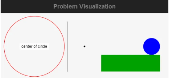
function arguments description and examples
IA.add intervalI, interval J Returns the sum of two intervals IandJ. IA.add([-1,2],[3,4]) = [2,6]
IA.sub intervalI, interval J Returns the difference of two intervalsIand J.
IA.sub([-1,2],[3,4]) = [-5,-1]
IA.mult intervalI, interval J Returns the product of two intervalsI andJ.
IA.mult([-1,2],[3,4]) = [-4,8]
IA.div intervalI, interval J Returns the quotient of two intervals I and J. If zero is an element ofJ, the function returns [0,0].
IA.div([-1,4],[2,4]) = [-0.5,2]
IA.div([-1,4],[-1,1]) = [0,0]
IA.add scalar scalarc, intervalI Returns the sum of a scalarc and an intervalI.
IA.add scalar(-1,[2,3]) = [1,2]
IA.mult scalar scalarc, intervalI Returns the product of a scalarcand an intervalI.
IA.mult scalar(-1,[2,3]) = [-3,-2]
IA.sq intervalI Returns the square of an interval I.
IA.sq([2,3]) = [4,9]
IA.sq([-3,2]) = [0,9]
IA.sqrt intervalI Returns the square root of an intervalI. Negative val- ues inI are limited from below by zero.
IA.sqrt([4,9]) = [2,3]
IA.sqrt([-7,4]) = [0,2]
IA.pow intervalI, integerp Returns the powerpof an intervalIwherepis assumed as positive integer.
IA.pow([-1,2],3) = [-1,8]
IA.min intervalI, interval J Returns the minimum of two intervalsIand J.
IA.min([1,4],[2,3]) = [1,3]
IA.max intervalI, interval J Returns the maximum of two intervals IandJ. IA.max([1,4],[2,3]) = [2,4]
IA.abs intervalI Returns the absolute value of an intervalI.
IA.abs([-1,4]) = [0,4]
IA.exp intervalI Returns the exponential of an interval I.
IA.exp([0,2]) = [1,7.389]
IA.log intervalI Returns the natural logarithm of an intervalI. If zero is an element ofI, the function returns [0,0].
IA.log([1,7.389]) = [0,2]
IA.sin intervalI Returns the sine of an intervalI.
IA.sin([0,3.141]) = [0,1]
IA.cos intervalI Returns the cosine of an interval I.
IA.cos([0,3.142]) = [-1,1]
IA.atan intervalI Returns the arctangent of an intervalI.
IA.atan([-2,2]) = [-1.107,1.107]
Table 1. List of all functions included in the interval arithmetic package (IA).
function arguments description and examples
PV.set size scalarsxL,xR,yL,yR,r Sets the plotting area to [xL, xR]×[yL, yR] with a ratio ofr=|y:x|. This is amandatoryfunction.
PV.set size(0, 10, 0, 4, 0.4);
PV.head stringS Draws the headline / caption of the plotting sur- face. This is amandatoryfunction.
PV.head("Problem Visualization");
PV.dot scalarsx,y Draws a simple black dot at (x, y).
PV.dot(5.0, 2.0);
PV.disc scalarsx,y,r, colorC Draws a disc with center (x, y), radiusr, and color C.
PV.disc(9, 2, 0.5, ’#0000FF’);
PV.circle scalarsx,y,r, colorC Draws a circumference / circle line with center (x, y), radiusr, and colorC.
PV.circle(2, 2, 1.8, ’#FF0000’);
PV.line scalarsx1,y1,x2,y2, colorC Draws a line from (x1, y1) to (x2, y2) with colorC.
PV.line(4, 0.5, 4, 3.5, ’#999999’);
PV.rect scalarsx,y,w,h, colorC Draws a rectangle starting at (x, y) with widthw, heighth, and colorC.
PV.rect(6, 0.5, 3.5, 1, ’#00A000’);
PV.text scalarsx,y stringS Draws a text box with textS, centered at (x, y).
PV.text(2, 2, "center of circle");
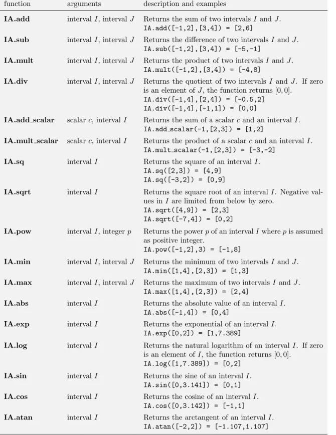
Table 2. List of all functions included in the problem visualization package (PV). Figure 5 illustrates the problem visualization applying all the examples given in this table.
3.4 Problem visualization
Finally, the problem visualization package (PV) can be used for the illustration of the prob- lem instance. To this end, acanvaselement with idcanvas Pis needed in theindex.html file as well as the function called plot problemin theproblem.jsfile. The argumentyof the function plot problem, see line 39 in Figure 6(b), is the current best-known solution x∗ throughout the algorithm.
Table 2 collects all functions which are included in the problem visualization package, see also Figure 5 and Subsection 3.5. Note that the two functions set size and head are mandatory.
3.5 Example problem
As a second example problem, we consider the two-dimensionalcenter problem. Here, we make use of the interval arithmetic package as well as the problem visualization package.
Assuming s given demand points A1, . . . , As on the plane, we would like to find a circle or disc with smallest radius which contains all these demand points leading to a two- dimensional problem, see Hamacher (1995) and references therein:
Figure 5. Problem visualization applying all the examples given in Table 2.
Given some demand points A1, . . . , As ∈R2, the center problem is to find the smallest disc with center X = (x1, x2) ∈ R2 containing these points. Thus, the problem is to minimize the objective function
f(x1, x2) = f(X) = max
k=1,...,skAk−Xk2 wherek · k2 is the Euclidean norm.
Figure 6 shows the source-code we used to solve the problem. The index.html file is the same as outlined in the examples before. Theproblem.jsfile contains the problem-specific source-code:
( 1 ) The mandatory parameters are defined in lines 1–3.
( 2 ) Theinit problemfunction is called once before the algorithm is running. Here, some demand points are randomly distributed in the unit square, see lines 7–11.
( 3 ) Lines 15–23 contain the source-code for the objective function.
( 4 ) Lines 27–35 contain the source-code for the calculation of the lower bounds. Here, we used the natural interval bounding operation, see Scholz (2012a), making use of the interval arithmetic package (IA).
( 5 ) Finally, lines 39–47 are to illustrate to problem making use of the problem visualiza- tion package (PV).
4 Example problems
Facility location problems are to find one or more new locations which, for instance, mini- mize the sum of some distances to existing demand points. Hence, we obtain a continuous objective function with only a few variables and, therefore, geometric branch-and-bound methods are popular solution techniques.
In this section we summarize some facility location problems as well as geometric problems which were solved by applying the suggested JavaScript branch-and-bound tool, see
www.mehr-davon.de/gbb/
(a)Source-code of theindex.htmlfile.
(b)Source-code of theproblem.jsfile.
Figure 6. Two-dimensional example of the JavaScript branch-and-bound tool: The center problem is solved inX= [0,1]×[0,1] with an absolute accuracy ofε= 10−6. The source-code can be downloaded from the homepage mentioned in the introduction.
4.1 The Weber problem
The two-dimensional Weber problem is to find a location for a new facility on the plane which minimizes the weighted sum of Euclidean distances to a given set of demand points.
If some weights are positive and others are negative, global optimization techniques are helpful solution algorithms, see for example Sch¨obel and Scholz (2010a) or Drezner et al.
(2001) and references therein.
Givensdemand pointsA1, . . . , As ∈R2 with weights w1, . . . , ws∈R, theWeber problem is to find a new facilityX= (x1, x2)∈R2 such that the new facility is close to demand points with positive weights and far away from demand points with negative weights. Thus, the problem is to minimize the objective function
f(x1, x2) = f(X) =
s
X
k=1
wk· kAk−Xk2
wherek · k2 is the Euclidean norm.
We applied the JavaScript branch-and-bound tool using the lower bounds as presented in Sch¨obel and Scholz (2010a).
4.2 The 2-median problem
The2-median problemor themultisource Weber problem is to find two new facilities on the Euclidean plane taking some given demand points into account, see Drezner (1984), Chen et al. (1998), or Sch¨obel and Scholz (2010a). Hence, we are dealing with a four- dimensional problem which can be formulated as follows.
Given s demand points A1, . . . , As ∈R2, the 2-median problem is to find two new facilities
X1 = (x1, x2) ∈ R2 and X2 = (x3, x4) ∈ R2 such that every demand point is served by its nearest new facility.
Hence, we want to minimize the objective function f(x1, x2, x3, x4) = f(X1, X2) =
s
X
k=1
min{kAk−X1k2,kAk−X2k2} wherek · k2 is the Euclidean norm.
We applied the JavaScript branch-and-bound tool using the lower bounds as presented in Sch¨obel and Scholz (2010a).
4.3 The 3-median problem
The 3-median problem is an extension of the 2-median problem to three new facilities, see Drezner (1984), Chen et al. (1998), or Sch¨obel and Scholz (2010a). Thus, we are dealing with the following six-dimensional problem.
Given s demand points A1, . . . , As ∈R2, the 3-median problem is to find three new facilities
X1 = (x1, x2), X2 = (x3, x4), and X3 = (x5, x6) such that every demand point is served by its nearest new facility.
Hence, we want to minimize the objective function f(x1, x2, x3, x4, x5, x6) = f(X1, X2, X3) =
s
X
k=1
j=1,2,3min kAk−Xjk2
wherek · k2 is the Euclidean norm.
We applied the JavaScript branch-and-bound tool again using the lower bounds as presented in Sch¨obel and Scholz (2010a).
4.4 The median circle problem
The median circle problem is to locate a circle so as to minimize the sum of distances between the circumference and some given demand points on the plane, see Brimberg et al.
(2009) or Sch¨obel and Scholz (2010a) for more details. Since every circle can be defined by its center and radius, we have a three-dimensional problem.
Givensdemand pointsA1, . . . , As∈R2, themedian circle problem is to find the center X = (x1, x2) and radius x3 ≥0 of a circle such that the sum of distances between the circumference and the demand points is minimized. Hence, we find the objective function
f(x1, x2, x3) = f(X, x3) =
s
X
k=1
kAk−Xk2 − x3
wherek · k2 is the Euclidean norm.
We applied the JavaScript branch-and-bound tool using the lower bounds as presented in Sch¨obel and Scholz (2010a).
4.5 The circle detection problem
Global optimization techniques can also be used in image processing to detect imperfect pictured shapes such as lines, circles, and ellipses. We here present the circle detection
problem although in the same manner it is also possible to detect other shapes such as lines or ellipses. Note that one first has to detect edges in a given image before the objective function can be formulated as follows, see Breuel (2003a), Breuel (2003b), or Scholz (2012a).
Assume a set of points A1, . . . , As ∈ R2, for example derived from an edge detection algorithm of an image. Than the circle detection problem is to find the centerX= (x1, x2) and radiusx3≥0 of a circle such that it fits to the given points. This problem can be modeled by a minimization problem with objective function
f(x1, x2, x3) = −
s
X
k=1
exp
−1
δ ·(kAk−Xk2−x3)2
+ C·x3 where k · k2 is the Euclidean norm and δ > 0, C ≥ 0 are some regularization parameters.
We applied the JavaScript branch-and-bound tool using the lower bounds as presented in Scholz (2012a).
4.6 The rigid body transformation problem
The two-dimensional rigid body transformation problem is to align two sets of points in the Euclidean space for which correspondence is known, see Eggert et al. (1997) and references therein. The transformation is defined by a rotation matrix and a translation vector.
Assume two sets of points
A1, . . . , As ∈ R2 and B1, . . . , Bs ∈ R2
in such a way that Ak is assigned to Bk for k = 1, . . . , s. Than the two-dimensional least squaresrigid body transformation problem is to minimize the objective function
f(x1, x2, x3) =
s
X
k=1
cos(x1) sin(x1)
−sin(x1) cos(x1)
·Ak+ x2
x3
− Bk
2
2
wherek · k22 is the squared Euclidean norm.
We applied the JavaScript branch-and-bound tool using the general bounding operation of second order, see Scholz (2012a). Note that the same procedure can also be applied to higher dimensional problems.
5 Conclusions
Geometric branch-and-bound methods are well-known solution techniques in deterministic global optimization. Our aim was to provide some software such that global optimization problems can be solved as simple as possible by the use of a geometric branch-and-bound algorithm. To this end, we suggested a JavaScript tool which includes the branch-and- bound algorithm as well as an interval arithmetic package and a problem visualization package. Hence, one basically only has to implement the objective function and a rule for the calculation of the lower bounds if one wants to solve a global optimization problem.
For the calculation of the required bounds, one might use the interval arithmetic package, see for example Subsection 3.5.
Although the JavaScript code can be used very easily and no further software is needed, the disadvantage is the run time since JavaScript code needs to be interpreted at any time the code is running. On the other hand, in Section 4 several examples from the field of location theory are given which can be solved efficiently for small and medium-sized problem instances. Furthermore, the code of the JavaScript tool as well as all example problems can be downloaded from the homepage mentioned in the introduction.
References
R. Blanquero, E. Carrizosa. 2009. Continuous location problems and big triangle small triangle: Constructing better bounds. Journal of Global Optimization,45: 389–402.
T.M. Breuel. 2003a. Implementation techniques for geometric branch-and-bound matching methods. Computer Vision and Image Understanding,90: 258–294.
T.M. Breuel. 2003b. On the use of interval arithmetic in geometric branch and bound algorithms. Pattern Recognition Letters,24: 1375–1384.
J. Brimberg, H. Juel, A. Sch¨obel. 2009. Locating a minisum circle in the plane. Discrete Applied Mathematics,157: 901–912.
P.C. Chen, P. Hansen, B. Jaumard, H. Tuy. 1998. Solution of the multisource Weber and conditional Weber problems by D.-C. programming. Operations Research,46: 548–562.
Z. Drezner. 1984. The planar two-center and two-median problems.Transportation Science, 18: 351–361.
Z. Drezner. 2007. A general global optimization approach for solving location problems in the plane. Journal of Global Optimization,37: 305–319.
Z. Drezner, K. Klamroth, A. Sch¨obel, G. Wesolowsky. 2001. The Weber problem. In Z. Drezner, H.W. Hamacher, editors, Location Theory - Applications and Theory, pages 1–36. Springer, New York.
Z. Drezner, A. Suzuki. 2004. The big triangle small triangle method for the solution of nonconvex facility location problems. Operations Research,52: 128–135.
D.W. Eggert, A. Lorusso, R.B. Fisher. 1997. Estimating 3-D rigid body transformations:
a comparison of four major algorithms. Machine Vision and Applications,9: 272–290.
H.W. Hamacher, 1995. Mathematische Verfahren der Planaren Standortplanung. Vieweg Verlag, Braunschweig, 1st edition.
E. Hansen, 1992. Global Optimization Using Interval Analysis. Marcel Dekker, New York, 1st edition.
P. Hansen, B. Jaumard. 1995. Lipschitz optimization. In R. Horst, P.M. Pardalos, editors, Handbook of Global Optimization, pages 407–493. Kluwer Academic, Dordrecht.
P. Hansen, D. Peeters, D. Richard, J.F. Thisse. 1985. The minisum and minimax location problems revisited. Operations Research,33: 1251–1265.
R. Horst, P.M. Pardalos, N.V. Thoai, 2000. Introduction to Global Optimization. Springer, Berlin, 2nd edition.
R. Horst, N.V. Thoai. 1999. DC programming: Overview. Journal of Optimization Theory and Applications,103: 1–43.
R. Horst, H. Tuy, 1996. Global Optimization: Deterministic Approaches. Springer, Berlin, 3rd edition.
A. Neumaier, 1990. Interval Methods for Systems of Equations. Cambridge University Press, New York, 1st edition.
F. Plastria. 1992. GBSSS: The generalized big square small square method for planar single-facility location. European Journal of Operational Research,62: 163–174.
H. Ratschek, J. Rokne, 1988. New Computer Methods for Global Optimization. Ellis Hor- wood, Chichester, England, 1st edition.
H. Ratschek, R.L. Voller. 1991. What can interval analysis do for global optimization?
Journal of Global Optimization,1: 111–130.
A. Sch¨obel, D. Scholz. 2010a. The big cube small cube solution method for multidimensional facility location problems. Computers & Operations Research,37: 115–122.
A. Sch¨obel, D. Scholz. 2010b. The theoretical and empirical rate of convergence for geo- metric branch-and-bound methods. Journal of Global Optimization,48: 473–495.
D. Scholz, 2012a. Deterministic Global Optimization: Geometric Branch-and-bound Meth- ods and Their Applications. Springer, New York, 1st edition.
D. Scholz. 2012b. Theoretical rate of convergence for interval inclusion functions. Journal of Global Optimization,53: 749–767.
H. Tuy. 1996. A general D.C. approach to location problems. In C.A. Floudas, P.M.
Pardalos, editors, State of the Art in Gloabal Optimization: Computational Methods and Applications, pages 413–432. Kluwer Academic, Dordrecht.
H. Tuy, F. Al-Khayyal, F. Zhou. 1995. A D.C. optimization method for single facility location problems. Journal of Global Optimization,7: 209–227.
H. Tuy, R. Horst. 1988. Convergence and restart in branch-and-bound algorithms for global optimization. Application to concave minimization and d.c. optimization problems.
Mathematical Programming,41: 161–183.

![Figure 3. One-dimensional example of the JavaScript tool: The objective function f (x) = sin(x) is minimized over the interval X = [0, 8] with an absolute accuracy of ε = 10 −6 .](https://thumb-eu.123doks.com/thumbv2/1library_info/4757940.1620798/9.892.146.746.133.491/dimensional-javascript-objective-function-minimized-interval-absolute-accuracy.webp)


![Figure 6. Two-dimensional example of the JavaScript branch-and-bound tool: The center problem is solved in X = [0, 1] × [0, 1] with an absolute accuracy of ε = 10 −6](https://thumb-eu.123doks.com/thumbv2/1library_info/4757940.1620798/15.892.151.745.170.967/figure-dimensional-example-javascript-branch-problem-absolute-accuracy.webp)
![Consider the functionf on the interval [0,1] defined by f(x](data:image/gif;base64,R0lGODlhAQABAIAAAP///wAAACH5BAEAAAAALAAAAAABAAEAAAICRAEAOw==)