Contextual Effects on the Vote in Germany A Multilevel Analysis

(1)

Veröffentlichungsreihe der Abteilung Institutionen und sozialer Wandel des Forschungsschwerpunkts Sozialer Wandel, Institutionen und Vermittlungsprozesse des

Wissenschaftszentrums Berlin für Sozialforschung ISSN 1615-7559

FS III 02-202

Contextual Effects on the Vote in Germany A Multilevel Analysis

Jan Pickery

Berlin, April 2002

Wissenschaftszentrum Berlin für Sozialforschung gGmbH (WZB) Reichpietschufer 50, D-10785 Berlin,

Telefon (030) 25 49 1-0

(2)

Zitierweise:

Pickery, Jan, 2002:

Contextual Effects on the Vote in Germany: A Multilevel Analysis.

Discussion Paper FS III 02-202.

Wissenschaftszentrum Berlin für Sozialforschung (WZB).

(3)

Zusammenfassung

Diese Arbeit befasst sich mit dem „alten“ Thema der Kontexteffekte beim Wahlverhalten.

Neue Techniken der Multi-Level-Analyse bieten ein mächtiges Instrument, mit dem regionale Einflüsse auf Wahlentscheidungen (neu) untersucht werden können. Die Multi- Level-Analyse wird auf deutsche Wahldaten angewendet und weist zwei Kontexteffekte nach. Die Arbeitslosenquote des Wahlkreises hat einen positiven Effekt auf die Unterstützung der SPD, was dem regionalen Äquivalent des Modells des „economic voting“ entspricht. Außerdem wirkt sich die allgemeine Stärke einer Partei in einem Kreis positiv auf die individuelle Entscheidung aus, diese Partei zu unterstützen. Dieses zweite Ergebnis bestätigt die Annahme, die als „Breakage“ bezeichnet wird. Beide Effekte zeigen, dass individuelle Wahlentscheidungen in Deutschland weiterhin regionalen Einflüssen unterliegen.

Abstract

This paper addresses the “old” topic of contextual effects on voting behaviour. Current multilevel analysis techniques provide a powerful tool to (re-)examine such regional influ- ences on individual voting decisions. We apply multilevel analysis to German electoral data. Our results prove evidence of two contextual effects. The unemployment level of the district has a positive effect on SPD support, which confirms the local equivalent of the economic vote model. Furthermore the global strength of a party in a district has a positive effect on the individual decision to support that party. This is a confirmation of what has been labelled as breakage. Both effects demonstrate the continuing impact of the locality on individual vote preferences in Germany.

(4)

(5)

Jan Pickery

Contextual Effects on the Vote in Germany A Multilevel Analysis

1 Introduction

Contextual effects on voting behaviour have been discussed for a long time. Theory and research about such contextual effects go back for at least 50 years. Political sociologists have often studied regional differences in voting behaviour and regularly tried to explain these differences in terms of contextual effects. New statistical methodologies, more par- ticularly multilevel analysis, allow for a readdressing of an old problem with a more powerful technique. Accordingly, in the last decade multilevel analysis has been used a few times for the analysis of voting behaviour (see e.g. Charnock, 1997 and Lubbers et al.

2000). In this paper we will apply multilevel analysis to German electoral data in order to find evidence (or absence) of contextual effects in Germany.

Germany is clearly a multiparty system with 4 (in the West) or 5 (in the East) parties achieving a ‘non-ignorable’ share of the votes.¹ Accordingly a multinomial logit model for multi-category responses is an appropriate tool to analyse voting behaviour. We will present a multilevel multinomial logit model that accounts for regional differences. As this model has not been applied widely up until now, especially not in political science, we will also describe the model itself. Applying that model, we will be able to demonstrate contextual effects on the vote. The interpretation of our results can also further clarify the nature of these effects.

In the next section we review theories and research about contextual effects on voting behaviour. In section 3 we describe the data and the variables used in our models. Section 4 presents the model we will use and the modelling strategy we will follow in our analyses.

Section 5 shows the results and section 6 concludes this paper.

1 We will analyse data from 1994. In the elections of that year, CDU/CSU, SPD, FDP, and Bündnis 90/Die Grünen achieved together 95.2% of the list votes (Zweitstimme) in former West-Germany, FDP being the smallest of these with 7.7%. In former East-Germany the PDS was also strong (19.8%). PDS, CDU, SPD, FDP, and Bündnis 90/Die Grünen covered together 97.6%, FDP again being the smallest with 3.5%.

(6)

2 Contextual effects on voting behaviour

Apparent geographical differences in voting behaviour have been studied for a long time.

These differences are however not necessarily the result of a contextual effect. Contextual effects are systematic differences in individual (voting) behaviour across environments that cannot be explained in terms of individual characteristics. When the differences between individuals in distinct regions account for the different voting behaviour, this variation cannot be interpreted as a contextual effect.

One of the first arguments for a contextual effect on the vote can be found in an early fifties study by Berelson, Lazarsfeld and McPhee (1954-1986). These authors show how voting is affected by social class, religious background, family loyalties and other factors.

They also argue that the personal network of an individual is very important in shaping his or her political preference. Individuals tend to comply with the general preference in their network. If preferences in the personal network are diverse though, an impact of the larger community would be possible. The surrounding majority would attract individuals with a diverse network. Over a long period of time this “breakage“ effect, as the authors call it, would result in an enduring general support for one party in a community. The strongest party tends to remain the strongest (ibid.: 100-101). This contextual effect can result in enduring geographical differences in the vote.

Several authors have studied this effect and provided further explanations for it. Klein and Pötsche (2000) cite three theories that have been used to explain the breakage effect:

party activity, identification or interaction theory. Party activity theory states that locally strong parties can and will carry on a more intensive election campaign, which further attracts new voters. According to the identification theory people identify with their area or region and consequently adopt subjectively acknowledged opinions and (majority) cli- mates in the region. Following interaction theory, connections between people from the same locality and their social interaction result in an impact of the locality on the individual vote. There is plenty of research on these explanations. Cutright e.g. (1963) focuses exclusively on local party activity. Analysing strong Democratic and Republican precints he does not find evidence for the hypothesis that the majority effect in voting behaviour exists as the consequence of political party activities. Fitton (1973) examines personal interaction in the street environment and Pattie and Johnston (1999) present some analyses that suggest that political conversation forms a distinct context within which people evaluate parties and decide who to support. Conversations with supporters of a particular party encourage respondents to vote for it too and discourage them from voting for other parties.

Whatever explanation of the effect is most valid, one can easily argue that the breakage effect is also transferable to a multiparty system, where there is no clear strongest party.

(7)

Interaction with partisans, party activity and identification will probably be stronger if a certain party is stronger in the region, regardless of whether this party has the (absolute) majority or not. One can also argue that this breakage effect should have decreased during the last decades due to individualisation and modernisation processes in society. As Klein and Pötsche (2000: 188-190) also point out people change local and social contexts more often nowadays and they are geographically more mobile. The result is a weaker identification and a wider interaction. Furthermore election campaigns are increasingly centrally organised and directed. Consequently Klein and Pötsche expect contextual effects on the vote to be less important, an hypothesis which is supported by their analysis. Their findings even seem to suggest that contextual effects have no significant importance anymore for individual voting decisions in Germany nowadays. Although the argument about the decreasing impact is clear and well founded, this last claim is probably too strong, since the authors do not take the categorical nature of the dependent variable fully into account.

Much attention has also been paid to class contextual effects on the vote (see e.g. Fisher, 2000). A class contextual effect implies that similar people vote differently depending on the class composition of their locality. People living in areas with a higher proportion of working class people would become more socialist, for example. Explanations for this effect are however similar to the explanations for the breakage effect. Fisher (2000: 348- 349) recites three explanations. Authors revert to social interaction, political socialisation or local political culture to explain the effect. As Fisher points out all explanations are in fact more shifting the focus from the class based aspect to a contextual effect associated with partisanship. As such this class contextual effect is rather a further explication of this breakage effect than something really different. His analysis proves evidence of an impact of the percentage employers or managers in a ward on an individual’s probability to vote Conservative. Also addressing class contextual effects, Andersen and Heath (2000) inves- tigate changes over time, like Klein and Pötsche. Unlike the results of those authors their results provide significant evidence for the continuing role of contextual social class on voting in Britain. “Paradoxically, while the relationship between individual’s own class positions and their voting decisions have declined over time, the relationship between their voting decisions and the class composition of the constituency in which they live has remained effectively stable.” (Andersen and Heath, 2000: 20).

Another focus in contextual voting research is on the effects of race, see e.g. Carsey (1995). A number of earlier American studies cited by Carsey have showed that white voters living in increasingly black counties and/or states become increasingly likely to vote in a manner considered hostile to black interests. As Carsey points out this effect contrasts with theories arguing for positive contextual influence on the behaviour of non-group members (like the class contextual effects theory). According to Carsey this contradiction

(8)

might be result of the level of aggregation. The effect of the class composition of a neighbourhood is probably different from the effect of the class composition of the state.

Carsey’s analysis that focuses on the neighbourhood shows indeed that the contextual effects of race are not so different from the contextual effects of factors like partisanship or social class. Addressing the same problem, Wright (1977) on the other hand finds a negative effect at the state as well as at the community level. Higher concentrations of blacks lead to more voting behaviour that can be interpreted as hostile to black. Lubbers et al.

tackle the same research problem in Europe. They use multilevel models to analyse extreme right voting behaviour and voting intentions in France, Germany and Flan- ders/Belgium (votes for “Front National,” “Republikaner,” and “Vlaams Blok” respec- tively). Individual variables in the analysis include occupational status, education and political attitudes. Regional variables are the unemployment level and the number of ethnic minorities. In all analyses they find increasing support for extreme right as the proportion of ethnic minorities gets higher (Lubbers and Scheepers, 2000; Lubbers and Scheepers, 2002; Lubbers, Scheepers and Billiet, 2000). They rely on the realistic conflict theory to explain ethnocentric attitudes and voting behaviour. According to this theory the competition over scarce resources causes intergroup conflict. Contextual conditions will reinforce this conflict. The competition along ethnic lines will be more severe in regions where immigration and unemployment levels are high or in regions where these numbers are increasing considerably. Existing ethnic boundaries are reinforced when the actual competition over scarce resources intensifies. To preserve a positive self-image outgroups are blamed for the increased competition and ascribed negative characteristics. Thus more severe competition may intensify social (contra-)identification and eventually may result in exclusionist reactions. It is precisely these exclusionist reactions that are proclaimed in extreme right wing programmes, which increase the attractiveness of the extreme right- wing in regions and times characterized by high competition. Competition theory can thus be used to explain contextual effects on right wing voting.

Pattie, Fieldhouse and Johnston (1995) also have an interest in local unemployment levels. According to the economic vote model, governments which preside over economic downturn will lose support, and perhaps power, while those who are in power during boom periods see their approval increase. These authors argue however that this theory and the analyses based on it tend to ignore the existence of regional and local variations in economic conditions. Therefore the main interest of their paper is the link between the local economic context and voting decisions. They find evidence of economic vote model at the local level: unemployment, while generally seen as an unimportant factor in voting decisions in national models, emerges as an important factor at the local level: its importance

(9)

as an influence on the vote is obscured in studies which fail to take into account its wide variations between different constituencies.

Kelley and McAllister (1985) finally represent the deviating opinion in this section. As they correctly point out, the social context in which a person lives is related to a wide vari- ety of politically relevant individual-level variables. To examine contextual effects, these factors have to be controlled for in the analysis, something which, according to these authors, hasn’t been done sufficiently in previous analyses. The final conclusion of their analysis is that the social characteristics of parliamentary constituencies have no significant effect on how their inhabitants vote, net of the voter’s own characteristics. Said differently:

social context has no significant importance in shaping voting behaviour in Britain once sufficient control variables are introduced.

In section 5 we will try to integrate these findings in multilevel analyses of German electoral data. Controlling for the relevant individual characteristics we will examine whether the regional variables (unemployment level, proportion of foreigners and general party support) have an effect on voting preferences, thus providing evidence for contextual effects. For class structure an indirect test with a proxy (employment structure) will be used. In the next section we further describe these variables and the individual characteristics in the analyses.

3 Data and variables in the models

We will use data from the pre-election study 1994 (ZA 2599)² and analyse the West-Ger- man part of it (“alte Bundesländer”). This choice is at least partly driven by practical considerations. First of all, we needed an indicator variable that for each respondent identifies the region, municipality or district he or she is living in. Not all election surveys in Ger- many have such a variable, but in the 1994 pre-election study it is available. Secondly the number of respondents is important as well. Recent post election surveys in Germany exist of about 2000 respondents. Due to very different voting behaviour and voting intentions, East- and West-Germany (the new and the old Bundesländer) should be separated in the analysis. When using a post-election study, the result would be a dataset of about 1000 respondents, which is very small for an multilevel model with a categorical response. We attempt to include the diversity of voting intentions in the analysis and therefore need a

2 The data used in this paper were made available by Zentral Archiv für Empirische Sozialforschung (ZA), Universität zu Köln. The data were originally collected by M. Berger, M. Jung, D. Roth from IPOS Mannheim and W.G. Gibowski from Bundespresseamt. ZA documented the data and prepared them for analysis. Neither ZA, nor the original collectors-researchers are responsible for the analyses or interpretations presented in this paper.

(10)

model with a multiple category response, which needs even more cases to be estimated.

So, the number of observations of the cumulated data set of the 1994 pre-election study (more than 10000 in West-Germany alone) was an important aspect. A disadvantage of this data set is a direct consequence of the nature of the survey. As it was a pre-election survey only voting intentions are known and not voting behaviour.³ Although a strong correlation between both can easily be assumed, results might have been more convincing with actual voting behaviour variables.

The voting intention is our dependent variable. Respondents were asked which candidate and which party they would vote for, if there would have been an election at the next sunday. We examine the party intention (list vote or “Zweitstimme”) and include the 4 major parties (CDU/CSU, SPD, FDP and Bündnis 90/Die Grünen) in the analysis.

The data set contains a bunch of individual level variables that can be used as explana- tory variables. We included sex, age, family status, education, employment status, employment category, confession and mass attendance. Al variables are transformed into one or more dummies. Female has the value 1 for women and 0 for men. Age was already categorised. We turned the 10 categories into 3 with 2 dummies as a result: young (-35) and old (+50). The middle in between these ages is thus the reference category. From family status we only retained married (or not). For education we grouped “no finished education” and primary school into low education, whereas final exam (“Abitur”) and everything above became high education. Employment status resulted in 5 dummies: full time occu- pied, half time occupied, unemployed, retired and houseman or housewife. The rest cate- gory is the reference. Employment category was transformed into 5 dummies: labourer, office worker, functionary, self-employed (or shopkeeper) and farmer. For confession we included Catholic and Protestant. Finally regular (mass) attender denotes respondents who go to church every Sunday or almost every Sunday.

Of the respondents in this data set also the district (“Kreis”) in which they live is known.

These administrative units will make up the geographical level of our analysis. This choice is also partly driven by practical considerations. A lot of information is collected at the district level. For some characteristics districts are the smallest geographical units for which information is available in official publications. A yearly publication of the German National Statistical Office (Statistisches Bundesamt) contains population and employment characteristics and geographical variables for all districts (Kreiszahlen). The 1995 and 1996 editions include the data for 1994 that we need. The unemployment level and the proportion of foreigners can be borrowed straightforwardly, but exact class contextual

3 The survey asked for previous voting behaviour in national and European elections. These variables are however not an alternative, since at least part of the respondents were not allowed to vote at these previous elections and, more importantly, that voting behaviour not univocally can be attributed to a region due to possible respondent removals.

(11)

variables, like the proportion of labourers and the proportion of employers or managers are not available. The publication does however describe the distribution of employees over different sectors. In these official statistics the working force is partitioned into 5 sectors:

resulting in 5 percentages as district variables. Sector 1 denotes the percentage working in agriculture, forestry and fishing, sector 2 the percentage working in industrial manufactories, sector 3 the percentage working in trade, traffic and news services, sector 4 the percentage working in other service companies and sector 5 the percentage working in gov- ernment services, private housekeeping and private organisations without profit aims. In our analyses we will sum up the sector 3 and sector 4 percentages since the last sector is somewhat unclear and they are probably indicators of a similar employment structure.

They are also positively correlated (0.45), whereas most of these sector percentages are (strongly) negatively correlated, just because they are percentages. Furthermore, the hypotheses would be the same for both the sector 3 and the sector 4 variable. The sector variables certainly do not exactly measure the class composition of a district. They can however partly be used as proxies. It is justifiable to assume a strong correlation between the proportion of labourers in a district and the proportion of the employed people working in industrial manufactories. A correlation between the percentage of higher level employees and the percentage working in sector 3 or sector 4 can also be expected, but it is probably not so strong. Apart from these two proxies, this employment structure partitioning allows for an examination of an additional class contextual effect. The CDU/CSU is his- torically the party of the farmers, more than any other party. Following class contextual theory one can hypothesize that the proportion working in sector 1 has a net effect on the probability to vote CDU/CSU, whether or not the respondent is a farmer him or herself.

The last district variable we need is the general support for the various parties. This can easily be measured by the election results. The results of the German general elections of 1994 for all districts are available in another publication of the Statistical Office (Bevöl- kerung und Erwerbstätigkeit) dedicated to this election. For this variable we look at the distribution of the list votes (Zweitstimme).

4 Method

To model information of various levels simultaneously multilevel analysis is used. Several multilevel models are possible, but during the last decade the random coefficients model has become the dominant one in the social sciences. In a random coefficients model, the variance of the dependent variable is decomposed into an individual and a group compo- nent. The specific trait of the model is not the functional form relating lower and higher

(12)

level variables, but rather a more sophisticated treatment of the error structure (DiPrete and Forristal, 1994: 334). In our analyses the variance in voting intention will be divided in a respondent and a district part and we will examine the effect of respondent and district variables on both variances.

The dependent variable is a four category variable. Such a variable can be analysed with a multinomial logit model. The multinomial logit model is a generalized logits model; it models different logits simultaneously. These logits are the logs of the fractions of the expected probabilities for the different categories of the dependent variable. The model is described e.g. in Stokes et al. (1995: 233-246). Goldstein (1995: 104-106) and Hedeker present the multilevel extension. Consider a 2-level model with two independent level 1 variables, a nominal response variable with t categories, and a varying constant at the higher level. Then the model is defined as:

) ( 0 2 ) ( 2 1 ) ( 1 ) ( ) 0

( ) (

log _t ^s ^s _ij ^s _ij ^s_j

ij s

ij = + x + x +u









 β β β

π

π (1)

In this formula: i indexes the level 1 units, the respondents, j the level 2 units, the districts, π_ij is the expected value (proportion) of the response for the ij^th respondent, β₀ is the intercept and β₁ and β₂ are the regression coefficients for the independent level 1 variables x_1ij and x_2ij, u_0j is the level 2 residual for the intercept, s = 1, …, t - 1. The formula clarifies that there are separate intercept parameters (β₀^(s)) and different regression parameters (β₁^(s) and β₂^(s)) for each logit. In fact t-1 logits are modelled and coefficients are fitted for each response category except from the base. When there are only 2 categories in the dependent variable, the model becomes an ‘ordinary’ logit model with a binomial response. This model can be extended by including more individual independent variables, independent district variables and/or random terms for the regression coefficients. (In the formula above there is no higher level variation for β₁^(s) and β₂^(s)). The model is completed by specifying a distribution for the observed response y_ij|π_ij. The standard assumption is that the observed proportions follow a multinomial distribution (details see Goldstein, 1995: 105).

As said before, in our analysis the level 1 units are the respondents, and the districts con- stitute the second level. The dependent variable is voting intention and t equals 4. We chose SPD as the base category and model 3 (t-1) logits: the log odds for an intended CDU/CSU vote instead of a SPD vote, the log odds for a FDP vote instead of a SPD vote and the log odds for a vote for die Grünen instead of a SPD vote. With random terms at the second level we allow for variation in these log odds between districts. We include respondent and district characteristics that can explain this variation.

(13)

This model can be implemented in programs like MIXNO and MlwiN.⁴

In the next section we will present the results of our MLwiN analyses. We will describe a succession of models. The first model will be a null model, a model without independent variables. That model allows us to assess the share of the variance that can be attributed to the district. Secondly we will enter the individual (respondent) variables. With this second analysis we examine whether there is still regional variation in voting intention when controlling for the individual characteristics. Subsequently we will include district variables thus trying to explain the remaining regional variance. We have 7 district variables to include in the models: 4 sectors (1 of them is a compound one), the district support for the parties and the unemployment level and the proportion of foreigners. These 7 variables are however strongly correlated. For the sector variables this is obvious as they sum up to 100%, resulting in negative correlations up to -0.730. But high (positive or negative) correlations can be observed for the other variables as well. So is the correlation between the proportion of foreigners and the sector 1 (agriculture) percentage -0,626 and amounts the correlation between the unemployment level and the share of SPD votes to 0.716. These high correlations will introduce multicolinearity in the analysis, which complicates interpretation. Coefficients will shift between models as section 5 shows. Therefore we do not include all district variables immediately. We start with the employment structure variables that allow for a (proxy) test of the class contextual effects. Next we include the unemployment level and the proportion of foreigners to test the local economic vote model and the contradicting hypotheses about the impact of the ethnic composition. As far as this last trait is concerned, it has to be noted that an extreme right or clearly anti-immigrant party is not included in our analysis. In order to explore the relationship between ethnic context and voting more thoroughly an inclusion of immigrant-hostile (extreme right) voting intentions would be necessary. That would however highly complicate our analysis because of the small number of extreme right supporters in the data set. In the final model we will include the general support for the various parties in the districts. We retained this variable for the

4 To fit multinomial models in MLwiN you need to use the multicat macros. The Windows facilities are rather small for these models (see Yang et al. 1999: 5-10). In MLwiN you choose the base category and create a new response variable, which is a transformation of the original response variable. It is a stack- ing of created dummies, which implies that the dataset is doubled, tripled, … according to the number of categories in the dependent variables: 3, 4, … So in our analysis the original data set is tripled. You also have to create new independent variables. These are products of the original predictor variables with the dummies for the response variable, which implies they get the value zero for a large part of the new dataset (2/3 in our analysis). This is a time consuming activity, but in a way it also clarifies the model you are fitting. For example you get a parameter estimate for each created predictor, which corresponds to the different regression coefficients for the variables for each logit. The assumption of the multinomial distribution is imposed by creating an artificial level 1. (This is done by the macros, you don’t have to do it yourself). The variances at level 1 and level 2 (the original first level) are constrained, but these constraints can be released to allow for extra multinomial variation. At level 3 the variation between the higher level units is measured. In our case we have to look at this level to evaluate district variation.

(14)

last model, since its effect is likely to be strong. In the analysis of Fisher (2000) for example, it was the higher level variable with the strongest effect. It also rendered all other higher level variables not significant. Since this breakage effect (or partisan reinforcement effect as Fisher calls it) is not an explanation in itself (see also section 2), it is worth examining the effect of the other district variables without this variable in the model.

5 Results of the analysis

The results of the analyses are reported in Tables 1 to 4. We present 4 different models to clarify the modelling strategy following the argument in the previous section. These tables also clarify that we chose SPD as the base category. We get parameter estimates for CDU/CSU, FDP and Die Grünen.

The first table presents the null model. In this model no independent variables are included. The model estimates an intercept for the three parties and decomposes the variance in the dependent variable in an individual and a district part. Remember that the first level is an artificial level imposed by the model assumptions.

Table 1: Results of the Null Model Fixed Part

CDU/CSU FDP Die Grünen

parameter s.e. parameter s.e. parameter s.e.

Level 1 – Individual

constant -0.023 0.030 -1.931 0.047 ** -1.314 0.044 **

* p < 0.05; ** p < 0.01

Random Part

parameter s.e. corr

Level 3 – District

σ²_CDU 0.131 0.021

σ_FDP/CDU 0.095 0.023 0.727

σ²_FDP 0.131 0.048

σDie Grünen/CDU 0.091 0.022 0.493

σDie Grünen/FDP 0.144 0.035 0.779

σ²_{Die Grünen} 0.260 0.047

-P/P 1.000 0.000 °

Level 1 – Multinomial Variance

σ²_e 1.000 0.000 °

° constrained

(15)

In a null model the intercepts reflect the distribution over the different categories of the dependent variable. All intercepts are negative, reflecting the position of the SPD as the party with the largest support in these data. The intercept for CDU/CSU is very close to 0 though and not significant, so support for both parties is about equal. But the number of respondents expressing their intention to vote for Die Grünen and even more for the FDP is—of course—considerably smaller.

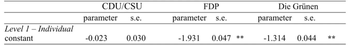
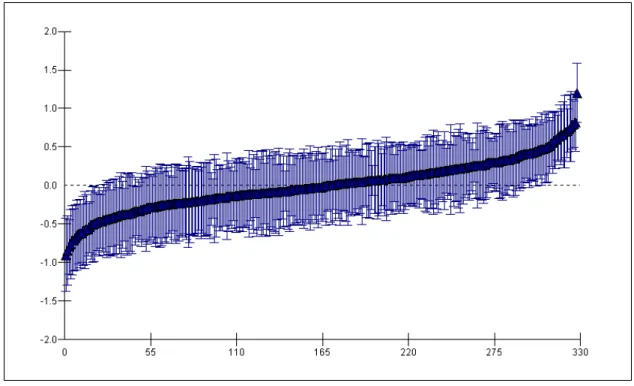
The random part at level 3 represents the variation across districts in general support for the three parties. More accurately, it reproduces the variances of the district residuals for the three logits (CDU/CSU|SPD, FDP|SPD, Die Grünen|SPD) and the covariances of these residuals. For the random part, significance tests based on standard errors are only indicative (Longford, 1999). But all variance and covariance terms are at least three times as large as their standard errors, except from σ²_FDP, which is still larger than 2.5 times its standard error. So it is legitimate to conclude that there is regional variation in recorded voting intention: support for the various parties is not equal in all districts. This result can be clari- fied further with a graph that shows the district residuals for a party and an interval that allows comparison with the other districts. Figure 1 displays this picture for Die Grünen.

Figure 1: District Residuals with Error Bars in the Null Model for Die Grünen

For all districts in the data set, the black triangle represents the residual for the logit Die Grünen|SPD. When looking at these residuals we can examine exceptional districts. At the far right hand side of the graph is a district with a very high residual. The logit Die

(16)

Grünen|SPD is much higher in this district than in all other districts. Moreover it is significantly higher than about 250 other district residuals. Its error bar shows no overlap with the error bars of the first 250 districts.⁵ Either Die Grünen have relatively very strong support in the district or support for the SPD is extremely low, or both. Apart from this exceptional district the graph shows that there are lots of districts with significantly residuals: about 40 districts at the left hand side of the graph have significantly lower residuals than about 40 districts at the right hand side. So this graph proves evidence for the district variation in the logit of interest.

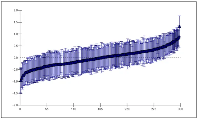
Apart from the variances, the random part of Table 1 also presents covariances and correlations of the residuals. All covariances are positive. That is not surprising since all parameters are relative to the SPD. It is highly likely that in districts where Die Grünen are doing relatively well compared to the SPD, other parties are also doing relatively well compared to the SPD, just because the SPD is probably not doing very well in those districts. This positive correlation can also be reproduced graphically. Figure 2 represents the correlation between the residuals for Die Grünen and those for the FDP.

The graph clearly shows the high positive correlation (0.779) between both residuals.

Looking at the 1994 election results in all districts there is also a rather strong positive correlation between both party results: 0.595. In districts where the FDP is performing well, Die Grünen also have stronger support. The correlation which results from this model is higher, because of the relative nature of the parameters. Of course the data are not exactly the same either: these data describe voting intentions in a sample and not the actual election results in the population.

In multilevel analyses often an intra-class correlation is used to express the share of variance which can be attributed to the higher level, in our analyses the district level. The assumption of a multinomial variance implies a level 1 variance of π²/3 (≈ 3.29) (see Snijders and Bosker, 1999; Hedeker, 2001).⁶ Doing so we can compute 3 intra-class correlations for the 3 logits. For Die Grünen for example, we have:

073 29 0

3 260 0

260

0 .

) . .

(

. =

+

5 These district errors are sample estimates with an amount of uncertainty. They have standard errors that depend on the number of respondents in the district and the between and within district variation (Gold- stein and Thomas, 1996: 161). Using these standard errors one can compare the residuals. Comparing districts involves however a series of statistical tests. For these test the intervals should be computed by multiplying the standard errors with ±1.4 (instead of ±1.96) for a significance level of α = 0.05 (see Goldstein and Healy, 1995, for details). A graphical representation of the residuals with the [±1.4] confi- dence intervals shows the significant non-overlap between districts.

6 π is the number denoted by the Greek letter (3.14159…). It should not be confused with the proportion in formula (1).

(17)

So about 7% of the variance in the logit Die Grünen|SPD can be attributed to the district level. The rest is variation between individuals. For CDU/CSU|SPD and FDP|SPD the share is only about 4%. Regional variation in intended voting behaviour is larger for Die Grünen than for CDU/CSU and FDP, but in general it is rather moderate. There is much more variation between individuals than between districts.⁷

Figure 2: District Residuals for Die Grünen and for the FDP in the Null Model

This first analysis proves evidence of geographical variation in voting intentions. It is however not a prove of a contextual effect on that intention. For such a prove it is necessary to control for relevant individual characteristics (see also the Kelley and McAllister argument in section 2). In the second analysis we include the independent respondent variables. The results are reported in Table 2. In this model, we only included the respondent variables that were significant for at least one of the three parties.

The fixed coefficients can be interpreted by transforming them into odds ratios. Female e.g. is a dummy (0 = male, 1 = female). Its parameter estimate for FDP|SPD equals -0.182, which corresponds with an odds ratio of 0.833 (= e^-0.182). Thus the odds FDP|SPD for women equal 0.833 times the same odds for men. In other words the FDP attract relatively

7 This computation is based on the variance estimates of the higher level residuals. As we do not take the covariance between the residuals into account, the intra-class correlations that are reported are approximate instead of really exact figures.

(18)

Table 2: Results of the Model with Individual Level Characteristics Fixed Part

CDU/CSU FDP Die Grünen parameter s.e. parameter s.e. parameter s.e.

constant -0.929 0.108 ** -2.136 0.197 ** -0.504 0.134 female -0.036 0.050 -0.182 0.094 * 0.194 0.070 *

young 0.089 0.060 -0.237 0.119 * -0.064 0.077 old 0.577 0.063 ** 0.631 0.112 ** -0.762 0.116 **

low education -0.232 0.054 ** -0.380 0.111 ** -0.555 0.092 **

high education 0.064 0.058 0.671 0.104 ** 0.787 0.077 **

married 0.076 0.046 -0.168 0.088 -0.333 0.069 **

full time 0.062 0.062 -0.027 0.120 -0.386 0.079 **

half time -0.253 0.090 ** -0.346 0.187 -0.098 0.115 retired 0.060 0.079 -0.458 0.153 ** -0.883 0.175 **

self employed 1.070 0.076 ** 1.322 0.116 ** 0.576 0.116 **

farmer 1.780 0.199 ** 1.829 0.302 ** 1.600 0.353 **

labourer -0.293 0.060 ** -0.462 0.137 ** -0.033 0.101 catholic 0.802 0.072 ** 0.323 0.127 * -0.205 0.087 *

protestant 0.274 0.070 ** 0.126 0.121 -0.529 0.085 **

regular attender 1.028 0.062 ** 0.517 0.121 ** -0.040 0.118

* p < 0.05; ** p < 0.01

Random Part

parameter s.e. corr

σ²_CDU 0.098 0.019

σ_FDP/CDU 0.067 0.020 0.705

σ²_FDP 0.090 0.042

σDie Grünen/CDU 0.098 0.020 0.659

σDie Grünen/FDP 0.106 0.030 0.758

σ²_{Die Grünen} 0.200 0.041

-P/P 1.000 0.000 °

σ²e 1.000 0.000 °

° constrained

fewer women. Similarly a positive coefficient means higher support among the respective category. Consequently, the CDU/CSU has relatively more support among older respondents, respondents who are self-employed or farmer and among catholic and protestant respondents and regular mass attenders. Respondents with a lower education, respondents

(19)

with a half time labour contract and respondents working as a labourer are relatively less likely to express a CDU/CSU voting intention. The FDP also has relatively more support among older respondents, self-employed respondents and farmers and among catholic respondents and regular mass attenders. Less support for the FDP is there among younger respondents, retired respondents, respondents working as labourers and respondents with a lower education. Die Grünen are doing relatively badly among lower educated respondents as well as among older respondents, married respondents, respondents working full time and retired respondents and among catholic and protestant respondents. They do however attract relatively more women, higher educated respondents, self-employed respondents and farmers.

For all parties we find a lot of significant predictors of the voting intention. Mind that these coefficients are partial and relative to the SPD. When comparing raw percentages for farmers for example, it will become clear that only the CDU/CSU has apparent support among farmers (although there aren’t that many anyway). It is mainly because the SPD is attractive to so few farmers (the difference in SPD support between non-farmers and farmers amounts to 30%) that the FDP and Die Grünen have a positive coefficient for this variable. The encountered relationships are however not of main interest here. The impact of including these variables on the random part of the model is more important for us. Apart from one covariance term in the model (σDie Grünen/CDU) all terms in the random part of the model have decreased considerably: if we don’t take that covariance into account, the average decrease is about 25%. We can show further evidence of this decrease with a similar graph for Die Grünen as the one presented after analysis 1. Figure 3 presents the district residuals and the error bars for analysis 2 for the logit Die Grünen|SPD.

The differences between Figure 3 and Figure 1 are rather small. There is for example still one outlier at the far right hand side with a residual which is a lot larger than the others. But in general the residuals have decreased somewhat. As a result of a similar decrease in standard errors though, the number of districts that differ significantly from each other remains apparently the same.

Figure 3 pictures the residual results of analysis 2 for Die Grünen, but these results are the same for all parties. The residuals have decreased, implying that part of the regional variation in voting intentions is due to individual characteristics. Support for the political parties varies across districts, but this variation is partly a consequence of differences between the individuals of the various districts. We can explain part of the variation with individual characteristics. On the other hand, after controlling for the individual variables in the model there are still differences between the districts. All variances and covariances at the district level remain substantial. Again, significance tests based on the standard errors are only approximate, but all ratios are considerably larger than two times their stan-

(20)

dard errors, except from σ²_FDP, for which the ratio parameter/standard error is close to 2.

Consequently, the results prove evidence for a geographical effect apart from individual characteristics: a contextual effect! In the following analyses we try to explain this contextual effect with district characteristics.

Figure 3: District Residuals with Error Bars for Die Grünen in the Model with Independent Individual Characteristics

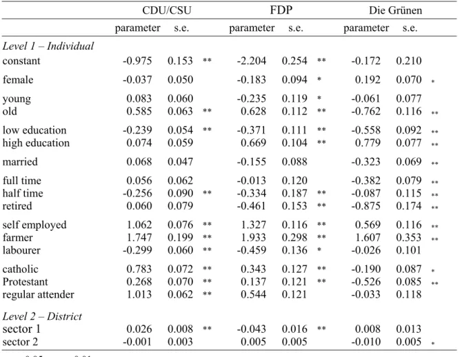
In analysis 3 we start by including variables that relate to the employment structure of the districts. In the official regional statistics the working force is partitioned into 5 sectors, resulting in 5 percentages as district variables. We added the sector 3 and sector 4 percentages up, since they both refer to the service sector. Of course it is impossible to include all 4 variables in the model, as they sum up to 100% and would introduce perfect multicolinearity. We tried various combinations of three sector variables, but the results were always equal. The sector 3/4 and sector 5 variables had no significant effects. Model 3 shows the results with sector 1, the percentage working in agriculture, forestry and fishing, and sector 2, the percentage working in industrial manufactories.

The fixed effects of the individual characteristics in this model remain the same as the ones in the previous analysis. The inclusion of higher level variables has no substantial impact on their size nor on their interpretation. The two employment structure variables have a significant contribution for at least one party. A higher sector 1 percentage in the district where a respondent lives increases his or her chance to report a CDU/CSU vote

(21)

Table 3: Results of the Model with Individual Characteristics and Employment Sectors Fixed Part

constant -0.975 0.153 ** -2.204 0.254 ** -0.172 0.210 female -0.037 0.050 -0.183 0.094 * 0.192 0.070 _* young 0.083 0.060 -0.235 0.119 * -0.061 0.077 old 0.585 0.063 ** 0.628 0.112 ** -0.762 0.116 _**

low education -0.239 0.054 ** -0.371 0.111 ** -0.558 0.092 **

high education 0.074 0.059 0.669 0.104 ** 0.779 0.077 _**

married 0.068 0.047 -0.155 0.088 -0.323 0.069 _**

full time 0.056 0.062 -0.013 0.120 -0.382 0.079 **

half time -0.256 0.090 ** -0.334 0.187 ** -0.087 0.115 _**

retired 0.060 0.079 -0.461 0.153 ** -0.875 0.174 _**

self employed 1.062 0.076 ** 1.327 0.116 ** 0.569 0.116 **

farmer 1.747 0.199 ** 1.933 0.298 ** 1.607 0.353 _**

labourer -0.299 0.060 ** -0.459 0.136 * -0.026 0.101 catholic 0.783 0.072 ** 0.343 0.127 ** -0.190 0.087 _* Protestant 0.268 0.070 ** 0.137 0.121 ** -0.526 0.085 _**

regular attender 1.013 0.062 ** 0.544 0.121 -0.033 0.118 Level 2 – District

sector 1 0.026 0.008 ** -0.043 0.016 ** 0.008 0.013 sector 2 -0.001 0.003 0.005 0.005 -0.010 0.005 _*

* p < 0.05; ** p < 0.01

Random Part

parameter s.e. corr

σ²_CDU 0.089 0.018

σ_FDP/CDU 0.074 0.019 0.830

σ²_FDP 0.086 0.041

σDie Grünen/CDU 0.101 0.019 0.729

σDie Grünen/FDP 0.108 0.029 0.776

σ²_{Die Grünen} 0.189 0.040

-P/P 1.000 0.000 _°

σ²e 1.000 0.000 _°

° constrained

(22)

intention over an SPD-vote intention; it decreases the relative chance for a FDP voting intention. If the share of the employed population working in sector 2 increases, the relative chance for a voting intention for Die Grünen decreases.

The first effect can be explained as a class contextual effect. The CDU/CSU can be labelled as the party that defends or (pretends to defend) the farmers' interests most. An increase in the respondent's chance to report a CDU/CSU vote intention in districts with more farmers can be interpreted as a consensual class contextual effect. This implies controlling for he or she being a farmer him or herself, which is the case as this individual variable is part of the model. The negative sector 1 coefficient for FDP is neither a confirmation, nor a falsification of this hypothesis. Another confirmation of a class contextual effect could have been possible for the parameter results for the percentage working in sector 2. The SPD is acknowledged as the labourers' party and following the class contextual theory one would expect that support for other parties decreases if the sector 2 percentage increases. The data confirm this hypothesis only for Die Grünen. We do not find a significant negative correlation between this percentage and support for CDU/CSU or FDP. This variable is only a proxy, the percentage working in sector 2 doesn't equal the percentage labourers, but a high correlation between these percentages can legitimately be expected, which led to the expectation of a negative effect of the sector 2 percentage for CDU/CSU and FDP. All in all our results provide only a weak confirmation for the class contextual effect hypotheses.

Nevertheless we found a few significant correlations between the employment structure and party preferences. As a result the inclusion of these variables also affects the random part of the model. The variances at the district level decrease, the covariances show a small increase though. Another small part of the variation between districts is explained with these variables. But again the similar decrease in standard errors would justify the conclusion that, controlling for all variables in the model, there are still differences between districts. In the next analysis, analysis 4 we try to explain these differences with the number of foreigners in the district and the unemployment level. The results of this analysis are reported in Table 4.

Also in model 4 the fixed effects of the individual variables remain roughly the same and their interpretation is entirely similar. The results for the district variables have changed though. This is an indication of multicolinearity between these variables and the other district variables, proportion of foreigners and unemployment level. The support for Die Grünen is still smaller among respondents living in a district with a higher percentage working in industrial manufactories are respondents are also less like to report an FDP vote intention, when living in a district with a higher percentage of the employed population working in agriculture, forestry and fishing. But the farmers-CDU/CSU class contextual

(23)

Table 4: Results of the Model with Individual Characteristics, Employment Sectors, Unemployment Level and Proportion of Foreigners

Fixed Part

constant -0.032 0.210 -0.966 0.369 * 0.283 0.304 female -0.042 0.050 -0.190 0.094 * 0.186 0.070 **

young 0.080 0.060 -0.228 0.119 -0.070 0.077 old 0.582 0.063 ** 0.629 0.112 ** -0.772 0.116 **

low education -0.232 0.054 ** -0.359 0.111 ** -0.553 0.092 **

high education -0.055 0.058 -0.649 0.104 ** 0.751 0.077 **

married 0.066 0.046 -0.154 0.088 -0.312 0.069 **

full time 0.043 0.062 -0.031 0.120 -0.398 0.079 **

half time -0.278 0.090 ** -0.356 0.186 ** -0.124 0.116 retired 0.056 0.079 -0.472 0.153 ** -0.880 0.175 **

self employed 1.027 0.076 ** 1.282 0.116 ** 0.518 0.117 **

farmer 1.646 0.198 ** 1.826 0.298 ** 1.397 0.375 **

labourer -0.286 0.060 ** -0.451 0.136 * -0.018 0.101 catholic 0.758 0.072 ** 0.329 0.126 ** -0.225 0.087 *

Protestant 0.289 0.070 ** 0.165 0.122 ** -0.502 0.085 **

regular attender 0.990 0.062 ** 0.490 0.122 -0.100 0.121 Level 2 – District

sector 1 -0.004 0.010 -0.092 0.021 0.007 0.016

sector 2 -0.004 0.003 0.001 0.005 -0.012 0.004 **

unemployment -0.086 0.010 ** -0.101 0.018 * -0.074 0.016 **

prop. of foreigners 0.003 0.006 -0.006 0.011 * 0.030 0.009 **

* p < 0.05; ** p < 0.01

Random Part

parameter s.e. corr

σ²_CDU 0.021 0.011

σ_FDP/CDU 0.000 0.000

σ²_FDP 0.000 0.000

σDie Grünen/CDU -0.004 0.013 -0.147

σDie Grünen/FDP 0.000 0.000

σ²_{Die Grünen} 0.062 0.027

-P/P 1.000 0.000 °

σ²e 1.000 0.000 °

° constrained

(24)

effect disappeared. In the current model there is even a negative, though not significant, parameter.

Apparently the structural variables, unemployment level and proportion of foreigners, change the previous results for the district variables. Apart from that they have clear effects themselves. The parameter for unemployment level is significantly negative for all parties.

So, controlling for all individual and district variables in the model, respondents are relatively less likely to support CDU/CSU, FPD and Die Grünen, when they are living in districts with higher unemployment. Consequently the SPD appears to be stronger and attracting more voters in districts with high unemployment! The parameter for the proportion of foreigners is only significant for Die Grünen. Support for this party is larger in districts with a larger number of foreigners.

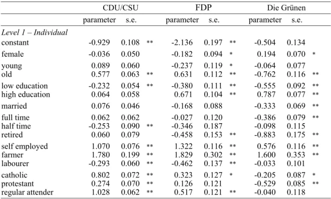
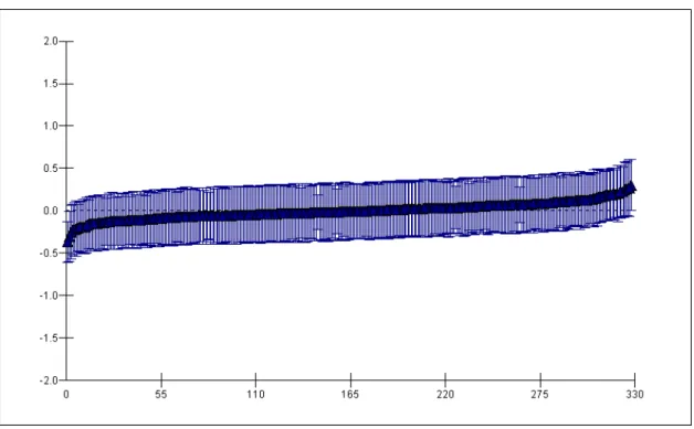
The impact of these two variables also becomes clear when looking at the random part of the model. Almost all variation between districts is explained. For the FDP this is liter- ally the case. The variance in FDP support between districts after controlling for all the variables in the model is estimated to be zero. But also the estimates of the variances of the CDU/CSU and the Die Grünen have decreased tremendously. Both variances amount to about twice their standard errors, and as such a significance test is only indicative, there is little reason to conclude additional differences between districts after the inclusion of all variables in the model. The residual plot with error bars for Die Grünen (Figure 4) proves graphical evidence.

When comparing districts at the left hand and right hand tails of the graph only very few significantly different districts can be discerned. The district with the highest residual shows no overlap with the districts with the three smallest residuals so they are significantly different, but that’s about it. For Die Grünen the inclusion of the last two variables decreased the unexplained variation between districts to an almost unimportant dimension.

For the other parties this is even more the case.

The results of analysis 4 show that the proportion of foreigners and the unemployment level are more important district predictors than the employment structure. This calls for an explanation. The SPD-unemployment effect is fully in line with the results of Pattie, Field- house and Johnston, reported in section 2. The SPD was in 1994 in the opposition and it appears to be stronger in regions with a higher unemployment level. This confirms the local equivalent of the economic vote model. Furthermore one can argue that the SPD is the party that used the unemployment problem most frequently as a campaign topic, much more than Die Grünen, who were also in the opposition at that time. An additional hypothesis might be that respondents living in a district with a higher unemployment are more aware of the problem. Therefore they might also be more likely to direct their voting behaviour or preference to a party which addresses this problem. This is a hypothesis

(25)

which is not fully testable with our data, but additional support is found in the fact that almost 58% of the SPD supporters in West-Germany chose unemployment as the most important problem in Germany at that time. This is the highest percentage of the four parties, the general mean amounts to 52%.

Figure 4: District Residuals with Error Bars for Die Grünen in the Model with Individual Characteristics, Employment Sectors, Unemployment Level and Proportion of Foreigners

The effect of the larger support for Die Grünen in districts with more immigrants is probably harder to explain. It is however remarkable that Die Grünen have the most explicit program when it comes to integration of foreigners (see Küchler, 1998). This party can probably be labelled as the most “immigrant-friendly.” Therefore we could attempt to explain this effect with the theories that have been used to explain context effects on Afro- American-friendly voting behaviour or—conversely—extreme-right voting behaviour in Europe. Our results seem to fit the positive contextual effect hypothesis, but it is again only a very partial confirmation. An even so plausible hypothesis could be that the Die Grünen voters tend to be more cosmopolitan (“städtisch und weltoffen,” ibid: 308) and therefore are more inclined to live in or to move to regions with more foreigners. As said before though a thorough examination of the relation between the ethnic composition of a regional unit and voting would also require an analysis of apparent anti-immigrant voting, which was technically unfeasible.

(26)

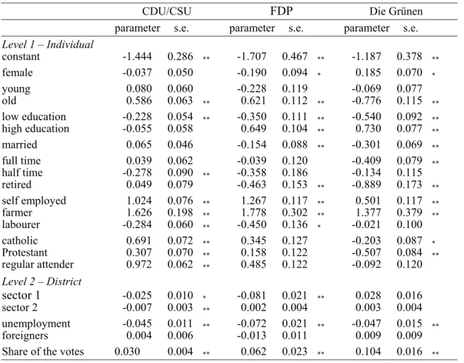
Table 5: Results of the Model with Individual Characteristics, Employment Sectors, Unemployment Level, Proportion of Foreigners and Party Support

Fixed Part

constant -1.444 0.286 ** -1.707 0.467 ** -1.187 0.378 **

female -0.037 0.050 -0.190 0.094 _* 0.185 0.070 _* young 0.080 0.060 -0.228 0.119 -0.069 0.077 old 0.586 0.063 ** 0.621 0.112 ** -0.776 0.115 **

low education -0.228 0.054 ** -0.350 0.111 ** -0.540 0.092 **

high education -0.055 0.058 0.649 0.104 _** 0.730 0.077 _**

married 0.065 0.046 -0.154 0.088 _** -0.301 0.069 _**

full time 0.039 0.062 -0.039 0.120 -0.409 0.079 **

half time -0.278 0.090 ** -0.358 0.186 -0.134 0.115 retired 0.049 0.079 -0.463 0.153 _** -0.889 0.173 _**

self employed 1.024 0.076 _** 1.267 0.117 _** 0.501 0.117 _**

farmer 1.626 0.198 _** 1.778 0.302 _** 1.377 0.379 _**

labourer -0.284 0.060 ** -0.450 0.136 * -0.021 0.100 catholic 0.691 0.072 _** 0.345 0.127 -0.203 0.087 _* Protestant 0.307 0.070 _** 0.158 0.122 -0.507 0.084 _**

regular attender 0.972 0.062 _** 0.485 0.122 -0.092 0.120 Level 2 – District

sector 1 -0.025 0.010 _* -0.081 0.021 _** 0.028 0.016 sector 2 -0.007 0.003 ** 0.002 0.004 0.003 0.004 unemployment -0.045 0.011 _** -0.072 0.021 _** -0.047 0.015 _**