Testing for Multivariate Equivalence with Random Quadratic Forms

Testing for Multivariate Equivalence with Random Quadratic Forms

Rafael Weißbach

Universit¨at Dortmund, Fachbereich Statistik,

Institut f¨ ur Wirtschafts- und Sozialstatistik, 44221 Dortmund, Germany

Correspondence: Rafael Weißbach, Institut f¨ ur Wirtschafts- und Sozialstatistik, Fachbereich Statistik, Universit¨at Dortmund, 44221 Dortmund, Germany

E-Mail: Rafael.Weissbach@uni-dortmund.de, Fax: +49/231/755-5284.

Abstract

Multivariate equivalence testing becomes necessary whenever the similarity rather than a difference between several treatment groups with multiple endpoints has to be shown.

This problem occurs in various applications, including bioequivalence or the comparison

of dissolution profiles. Therefore, several tests have been suggested during the last decade

for the assessment of multivariate equivalence. Recently Munk & Pfl¨ uger (1999) proposed

to test ellipsoidal instead of rectangular hypotheses as it is current practice in many ap-

plications. In this paper we provide several asymptotic tests for ellipsoidal equivalence

which are compared numerically with competitors suggested by Brown, Cassella & Hwang

(1995) and Munk & Pfl¨ uger (1999). We find that the proposed tests are superior (up to

90%) to both tests with respect to power. In addition, a simulation study reveals the sug-

gested tests as robust against violation of normality. These tests are very simple to apply,

because inversion of confidence regions is avoided. Asymptotic formulas for the power

function and sample size determination are given. Finally, all procedures are compared

in two data examples.

keywords and phrases: hypotheses testing, multivariate bioequivalence, multiple end- points, confidence inclusion rules, equivalence, Hotelling’s T

test, equivariance, boot- strap, quadratic forms, power function.

1 Introduction

Recently, testing of multivariate equivalence hypotheses has become a field of certain interest, mainly motivated by the problem of assessing multivariate bioequivalence, i.e. the assessment of a similar rate and extend of absorption in the blood circulation (cf. Chow

& Liu (1992) for a survey) of several pharmacokinetic characteristics of two different formulations of a drug. We refer to Brown, Cassella & Hwang (1995), Hsu, Lu

& Chan (1995), Chinchilli & Elswick (1997) or Wang, DasGupta & Hwang (1999) for a discussion and several tests for the multivariate bioequivalence problem.

However, the multivariate equivalence problem is not solely restricted to bioequivalence assessment as the following example from neurophysiology shows. For further applications in environmental or managerial science cf. Erickson & McDonald (1995), Dixon (1998) or McBride (1999).

Example 1. Exteroceptive suppression (cf. Schoenen (1993)), ES, of temporalis mus- cle activity is the electrophysiological correlate of the jaw-opening reflex. ES consists itself in two further components ESM and ESP, the monosynaptic and polysynaptic sup- pression. Steinhoff et al. (1996) investigated the influence of epilepsy on ES in a study with 20 healthy volunteers and 31 patients with epilepsy. The conjecture, that ES could be possibly influenced by epilepsy was essentially based on the observation that Parkinson’s disease and chronic headache seem to cause an effect on ES (Nakashima et al. (1990)). This analogy, however, was never based on solid physiological grounds.

Therefore, it was the aim of Steinhoff et al.’s (1996) study to show that this con-

jecture cannot be supported by the data. To this end several two sided t tests for the

null hypotheses of no difference were performed, each resulting in p-values larger than

0.8. However, this does not imply the rigorous assessment of similarity at a controlled error rate between the control and epileptic group as pointed out by Steinhoff et al.

(1996). An explorative data analysis suggests to assume a bivariate (ESM, ESP) normal model with the same covariance structure for the epileptic (E) and control group (C), respectively (cf. Munk & Pfl¨ uger (1999) for the raw data)

X

∼ N

(θ

, Σ) ˜ i = C, E and j = 1, . . . , n

with n

= 19, n

= 31.

The following (with pooled variance estimator for the ESP and ESM values, respectively) estimators for the mean difference and covariance matrix are obtained

X := ¯ X

− X ¯

=





− 0.0586

− 0.3325



 and Σ = ˆ





0.8526 0.0188 0.0188 1.3525



 .

In the following we present tests in order to assess that there is no ’relevant difference’

of the means between the reference group and the epilepsy group, for ESM and ESP , respectively. Hence, it follows that ES is not an appropriate diagnostic tool for epilepsy or the success of a particular therapeutic method as conjectured by Steinhoff et al.

(1996). To this end it is required to show at a controlled error rate that θ

≈ θ

.

According to various definitions of similarity several tests for multivariate equivalence were suggested in the literature during the last 5 years. Most of these tests are designed for rectangular hypotheses under a normal assumption (cf. Berger (1982), Berger &

Hsu (1996), Roy (1996) or Wang, DasGupta & Hwang (1999)). These authors provide several tests in order to assess that a multivariate mean θ = (θ

, . . . , θ

) ∈ R

is contained in a hyperrectangle, i.e. for the hypotheses

H : θ ∈ Θ

= { θ : ∃ i : | θ

| > ∆ } vs. K : θ ∈ Θ

= { θ : max

i=1,...,p

| θ

| ≤ ∆ } . (1)

The most popular tests for (1) are based on the intersection union principle applied to confidence interval inclusion rules (Berger & Hsu (1996)). These tests are simple to perform and well established in applications. They may have the disadvantage to be rather conservative (resulting in a low power) when the number of endpoints p increases as pointed out by Hwang (1996) and Munk & Pfl¨ uger (1999). The definition of equivalence in terms of the maximum norm is, of course, not the only possibility to formalize similarity. Therefore, Munk & Pfl¨ uger (1999) suggested to consider ellipsoidal hypotheses

H : θ

Aθ > ∆ vs. K : θ

Aθ ≤ ∆, (2)

for a positive defintite matrix A > 0. This is, e.g., in accordance with a measure of equivalence recommended by the FDA (1997) for testing equivalence of dissolution pro- files, i.e. the proportion of a tablet dissolved against time. For a discussion of recent methodology in dissolution profile testing we refer to O’Hara et al. (1997), Shah et al. (1998) or Sierra-Cavazos & Berger (1999). Because these hypotheses cannot be represented as the intersection resp. union of several one-dimensional hypotheses the intersection union principle (cf. Berger & Hsu (1996)) or related methods cannot be applied and different testing methodology is required. Here, the general testing princi- ple of Aitchison (1964) by inverting 1 − α confidence regions is applicable. This leads, however, in general to very conservative tests (Munk (1994), Berger & Hsu (1996)).

For general hypotheses this technique was improved by Brown et al. (1995) and for convex alternatives by Munk & Pfl¨ uger (1999).

This paper is organized as follows. In Section 2 we state the precise model for the test. In

Section 3 we review on existing methods for the assessment of multivariate equivalence and

discuss various new tests for the hypotheses (2). Our approach is based on the asymptotic

normality of the centered quadratic form X

AX − θ

Aθ (after normalizing by the sample

size). In Section 4 we present the results of a Monte Carlo study on size and power which

shows that the normal approximation yields rather liberal tests, i.e. the nominal level is exceeded. In order to improve the accuracy of the normal approximation several finite sample approximations are investigated including various Box - type χ

approximations and bootstrap tests. We found that the bias corrected accelerated boostrap method (Efron & Tibshirani, 1993) represents a good compromise between a very powerful method and a method which maintains its nominal level with high accuracy. In particular, differences in power up to 90% compared to Brown, Casella & Hwang’s (1995) and Munk & Pfl¨ uger’s (1999) test were observed. Furthermore, simulations show that the new test is very robust against violation of normality.

Finally, in Section 5 we compare all methods by reanalyzing the data set in Example 1 and an example from Chinchilli & Elswick (1997), who investigated the multivariate bioequivalence of two different formulations of Ibuprofen.

The paper closes with a discussion and summary section where also formulae for comput- ing sample size and power are given.

2 Model and testing problem

We restrict ourselves for the moment to i.i.d. observations coming from a normal model.

Generalizations to the two sample comparison and other designs will be discussed later.

We mention also that our results are asymptotically valid under very weak assumptions on the error distribution which is in contrast to existing methods for testing multivariate equivalence. This will be made precise in the next section.

Let throughout the following X

, · · · , X

∼ N

(θ, Σ) independent random variables, which ˜ follow a p-variate normal distribution with mean θ ∈ R

and covariance ˜ Σ ∈ R

which is assumed to be positive definite, ˜ Σ > 0. Sufficient statistics are the mean

P

i=1

X

=: X and the covariance estimator ˆ Σ =

P

i=1

(X

− X)(X

− X)

. It follows that X ∼ N

(θ, Σ),

and ˆ Σ ∼ W

(Σ) (here Σ =

Σ and ˜ d = n − 1 ≥ p) are independently distributed

according to a multivariate normal distribution with unknown mean θ ∈ R

and unknown covariance structure Σ and a Wishart distribution with d degrees of freedom, respectively (Anderson (1984)). Throughout the following we may consider w.l.o.g. instead of the testing problem in (2) the standardized problem

H : θ

θ > 1 vs. K : θ

θ ≤ 1. (3)

This can be achieved in (2) for any A > 0 by a transformation of the data X

into

X

= 1

√ ∆ A

X

(4)

because A > 0 allows a unique decomposition as A

A

= A, A

a symmetric matrix.

In order to keep notation simple we will write in the following X

instead of X

.

Before we consider the construction of several tests for (3), we find it pertinent to recall briefly the discussion in (Munk & Pfl¨ uger (1999)) concerning the choice of ellipsoidal hypotheses instead of rectangular hypotheses as in (1). In most applications θ will be the difference of two means θ = θ

− θ

which have to be shown to be equivalent (cf.

Example 1). For example, drug authorities, such as the FDA, currently require that

in a single dose bioequivalence study of oral drug formulation average bioequivalence is

shown with respect to both, AUC and C max. We mention that the criterion of aver-

age bioequivalence which focuses on the comparison of means solely, has been criticised

by various authors (cf. Hauck & Anderson (1992) or Schall (1995) among many

others) and different bioequivalence criteria (various types of population and individ-

ual bioequivalence) have been suggested. This is highlighted in a recent draft guidance

for industry entitled ”Average, Population and Individual Approaches to Establishing

Bioequivalence” (U.S. Dep. of Health and Human Services, Food and Drug

Administration, CDER, Rockville, MD (1999)). In the present paper, however,

we focus only on average bioequivalence, simply denoted as bioequivalence. According to the FDA guidance, bioequivalence may be claimed if every univariate comparison of the pharmacokinatic parameters AU C, T max, or C max allows one to declare bioequivalence at level of significance α = 0.05 (e.g. Guidance for Industry: In Vivo Pharma- cokinetics and Bioavailability Studies and in Vitro Dissolution Testing for Levothyroxine Sodium Tablets, U.S. Department of Health and Hu- man Services, CDER (1999)). To our knowledge up to now all approaches focus on hypotheses as in (1), i.e. bioequivalence is declared if each of the components of the difference of the mean vector is close to zero. We believe, however, that often the con- sideration of quadratic forms Q

(θ) = θ

Aθ as a distance measure is more appropriate (cf. Munk & Pfl¨ uger (1999) for a discussion). Here the region of equivalence is the ellipsoid Q

= { θ : Q

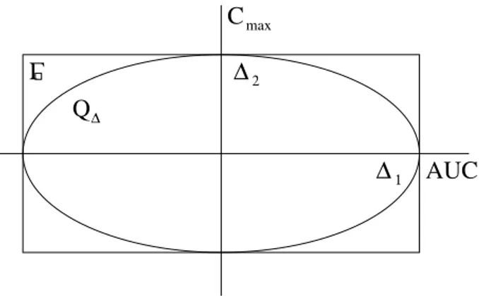
(θ) ≤ ∆ } where ∆ denotes a fixed tolerance bound (cf. Figure 1).

Γ Q

∆

∆

∆

1 2

C

AUC

max

Figure 0: Ellipsoidal (Q

) and rectangular hypotheses (Γ

) in the case p = 2

Interestingly, for the anaylsis of dissolution profiles, the FDA (1997), recommends ellip- soidal hypotheses completely analogous to (3). Methods for this problem are discussed in Moore & Flanner (1996), O’Hara et al. (1997) and Shah, Tsong, Sathe

& Mia (1998). For example, the f

method proposed in Moore & Flanner (1996)

requires weights ω

which corresponds to the eigenvalues of the matrix A in (2). Ma

et al. (2000) performed a simulation study for bootstrapping the f

-statistic with the

percentile method and found quite reasonable performance of the resulting test.

3 Tests

In this Section we will discuss several testing procedures for the multivariate equivalence problem (3). This includes tests already suggested in the literature and various new tests.

We restrict our representation to the case of an i.i.d. sample X

, · · · , X

. Generalizations to the two sample comparison with independent samples, such as required in Example 1, are straight forward and discussed in Example 1 in Section 5.

3.1 Confidence inclusion rules

A classical principle due to Aitchison (1964) states that for any confidence set C

(X, Σ) ˆ for θ at level 1 − α the region

A(Θ

) = { X : Θ

∩ C

(X, Σ) ˆ 6 = ∅}

defines the acceptance region of a test for H : θ ∈ Θ

against K : θ ∈ Θ

, Θ

∩ Θ

= ∅ , at level α because

P

(θ / ∈ C

(X, Σ)) ˆ ≤ α.

Hence, if Θ

:= { θ ∈ R

: θ

θ ≤ 1 } , the p-dimensional sphere, the following rule constitutes a test at level α for the hypothesis (3):

ψ

(X, Σ)) = ˆ







1 : C

(X, Σ) ˆ ⊂ Γ

0 : else

.

Munk & Pfl¨ uger (1999) showed, that if the confidence set obeys certain equivariance properties and the alternative K is convex (which is, of course, the case in the present setting) it is possible to improve Aitchison’s (1964) result because then the resulting level of the test is α/2. The level α/2 is sharp, i.e. it cannot be improved in general. This leads to the following test which results from inverting Hotelling’s confidence set.

3.1.1 Hotelling’s T

confidence set

In a first step we invert Hotelling’s T

test (cf. Anderson, (1984)) for H : θ = θ

with test statistic

T

:= d(X − θ

)

Σ ˆ

(X − θ

) (5)

which yields the (1 − α) confidence set

C

:= { θ

: T

≤ f

} , (6)

where f

=

F

(α) and F

denotes a central F -distribution with µ and ν degrees of freedom. Theorem 2.1 in Munk & Pfl¨ uger (1999) yields that

ψ

(X, Σ) = ˆ







1 : C

(X, Σ) ˆ ⊂ Θ

0 : else

constitutes a test at level α. Observe, that the confidence region required for the test ψ

has confidence coefficient 1 − 2α and not 1 − α.

3.1.2 Brown-Casella-Hwang’s confidence set

Another candidate for the confidence inclusion rule is the confidence set constructed by Brown et al. (1995). The reasoning behind their approach is to minimise the expected volume at a preassigned parameter point θ

, which can be assumed w.l.o.g. as θ

= 0.

Originally, this confidence set was constructed for the case of know variance Σ, resulting in the confidence set

C

(X, Σ) := { θ : (θ

Σ

θ)

≤ z

+ XΣ

θ (θ

Σ

θ)

} ,

where z

is the upper α quantile from a univariate standard normal distribution. For the case of unknown covariance we will throughout the following simply replace Σ by the estimator

Σ. Hence denote ˆ

ψ

(X, Σ) = ˆ







1 : C

(X,

Σ) ˆ ⊂ Θ

0 : else

as the according equivalence test. Note, that the BCH-confidence set does not share the equivariance property (like the Hotelling’s T

confidence set) required for application of Munk & Pfl¨ ugers (1999) Theorem 2.1 and hence the 1 − 2α-adjustment is not valid.

Other confidence regions and generalizations of this approach to nonnormal errors can be found in DasGupta, Gosh & Zen (1995), Wang, DasGupta & Hwang (1999) or Roy (1996).

3.2 Testing with quadratic forms

3.2.1 The δ -method

The most direct way to construct a test for (3) is to estimate in a first step θ

θ by

|| X ||

= X

X and then reject the hypothesis for || X ||

too small. The main difficulty

encountered with this approach is the effective determination of the distribution of || X ||

. Observe, that (cf. Mathai & Provost (1992))

|| X ||

=

X

j=1

λ

(U

+ b

)

(7)

equals in distribution a sum of weighted noncentral χ

random variables where U

∼ N

(0, 1) are i.i.d., j = 1, . . . , p. The weights λ

, j = 1, · · · , p, are the eigenvalues of Σ and

b = (b

, · · · , b

)

= 1

√ n P

Σ

θ

, (8)

where P denotes an orthogonal matrix such that

P

ΣP ˜ = diag(λ

, . . . , λ

). Here diag(λ

, . . . , λ

) denotes a p × p diagonal matrix with diagonal elements λ

, . . . , λ

. This representation highlights the difficulty to determine the exact distribution of || X ||

be- cause particularly the estimation of the eigenvalues of Σ causes serious problems. There- fore, we investigate in the following various approximations of the distribution of || X ||

. The simplest method of approximation is the C.L.T.

Theorem 1. Let X

, · · · , X

∼ F be an i.i.d. sample from a p-variate distribution F , s.t.

EX

= θ ∈ R

, Σ = ˜ Cov[X

] > 0 and E || X

||

< ∞ . Then we have for any consistent estimator Σ ˆ of the covariance Σ ˜

T

:= √

n X

X − θ

θ p 4X

ΣX ˆ

=

⇒ N (0, 1) for θ 6 = 0, as n → ∞ .

Proof. Apply the δ-method and the multivariate C.L.T. (cf. Serfling (1980)) in order to conclude that

√ n(X

X − θ

θ) =

⇒ N(0, 4θ

Σθ) for ˜ θ 6 = 0.

Observe, that from Kolmogorov’s strong law of large numbers it follows that X

ΣX ˆ −→

θ

Σθ. Now the assertion follows from Slutzky’s Lemma (Chow & Teicher (1997)). ˜

2 From Theorem 1 we obtain the following asymptotic test

ψ

(X, Σ) = ˆ







1 : √

n(X

X − 1)/ p

4X

ΣX ˆ ≤ z

0 : else

for the problem (3), where z

denotes the lower α-quantile of the standard normal distri- bution. In the next section we will demonstrate in a Monte Carlo study that this tests improves essentially on the power of the confidence region inclusion rules discussed in the last subsection. However, it turns also out that the normal approximation yields a rather liberal test (i.e. the nominal level is exceeded) and hence we investigate in the following various finite sample approximations.

Remark 1. In particular, when θ is close to zero, the distribution of T

is skewed. For

θ = 0 the asymptotic normality in Theorem 1 even fails to hold. Instead, the distribution,

after multiplication by n

once more, is a sum of weighted χ

distributions (cf. (7)

again). To account for this skewness we used an idea dating back to Box (1954) where

the approximation by a scaled χ

-distribution gχ

with random degrees of freedom f and

scaling parameter g is suggested. However, simulations for the approach revealed sizes of

up to three times the level for small sample sizes as 10. As a consequence, we refrain from

displaying the results. Increasing the number of fitted moments by using a non-central

χ

-distribution did not show to improve the size.

3.2.2 The bootstrap

Another option is, of course, to work with bootstrap approximations. The bias corrected and accelerated bootstrap (BC

) is investigated with

ψ

(X

, · · · , X

) =







1 : (X

X

)

≤ 1 0 : else

where α

= Ψ(ˆ z

+

1(1−^α₂)

1−ˆa(ˆz0+Ψ⁻¹(1−^α₂))

) with ˆ z

= ] {

} and the acceleration ˆ a =

Pn

i=1(ϑi−ϑ_·)² (Pn

i=1(ϑi−ϑ·)³)³²

. Here ϑ

is a jackknifed version of X

X, s.t. X

omitted. Further ϑ

denotes the empirical mean of the ϑ

’s i = 1, . . . , n and Ψ the c.d.f. of a standard normal r.v..

For more details see Efron & Tibshirani (1993).

Remark 2. Additional to the bias corrected and accelerated bootstrap we used the per- centile bootstrap (Efron & Tibshirani (1993)). As in the case of the χ

-approximations we found a sizes for our small sample situation of 10 observations which are clearly - up two-and-a-half times - above the level. Again, we refrain from displaying the results.

4 Simulation study

In this section we report on a Monte-Carlo study for the testing problem (3) which was conducted using the random generator of SAS/IML, internal programming language of the statistical software SAS, Version 6.12 and 8.03. In each scenario 10000 Monte-Carlo simulations were performed. The nominal level is always chosen as α = 0.05. In our first scenario 20 bivariate normal random variables were generated where the covariance was assumed as

Σ = ˜





1

8

−

−



 .

The power curve was obtained by cubic B-spline interpolation (in the alternative K) between the grid points







θ : θ =



 θ

θ



 =





i 10

0



 , i = 1, . . . , 10





 .

The number of bootstrap replications for the BC

bootstrap was n

= 300, respectively.

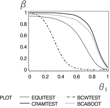
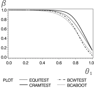
Power curves for all tests discussed in the last section are shown in Figure 1. Note, that θ

= 1 corresponds to the point (1, 0)

on the boundary of the null hypotheses (3), whereas smaller values of θ

are in the alternative of equivalence. If for the BC

bootstrap the argument of Ψ

( · ) in the calculation of ˆ z

was zero, we have dropped this value. This occurred in less that 1% of all cases.

Figure 1: Power curves of the δ-method (CRAMTEST), Munk & Pfl¨ uger’s (1999) test (EQUITEST), the Brown et al. (1995) test (BCWTEST), and the BCA bootstrap (BCA- BOOT) for n = 20, normal error and 10.000 simulations. The nominal level was α = 0.05.

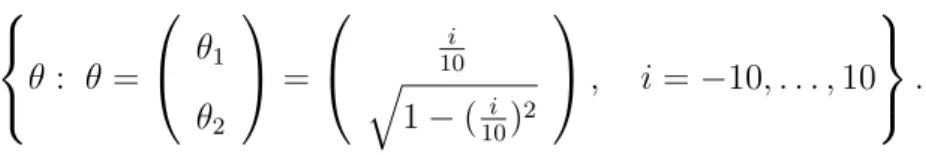
The next simulation study was performed in order to investigate the actual size of all

tests more detailed. Therefore in Figure 2 the actual level of all tests is displayed for the

following boundary points of the hypothesis H in (3)







θ : θ =



 θ

θ



 =





i 10

q

1 − (

)



 , i = − 10, . . . , 10





 .

under the same distributional assumptions as in Figure 1. Again cubic B-spline interpo- lation is used to interpolate between these grid points.

Figure 2: Actual size of the tests where || θ || = 1 and θ

> 0.

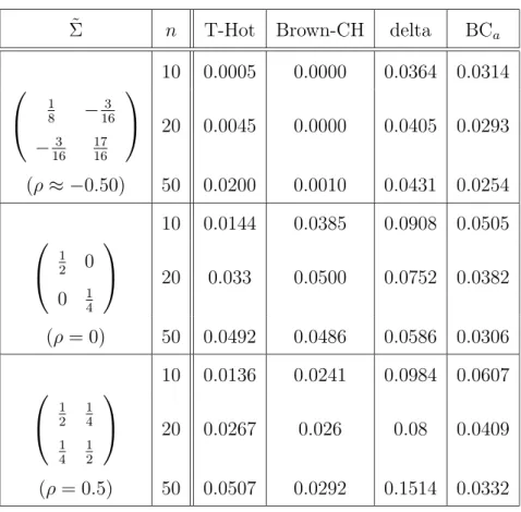
Σ ˜ n T-Hot Brown-CH delta BC

10 0.0005 0.0000 0.0364 0.0314





1

8

−

−



 20 0.0045 0.0000 0.0405 0.0293 (ρ ≈ − 0.50) 50 0.0200 0.0010 0.0431 0.0254 10 0.0144 0.0385 0.0908 0.0505





1

2

0

0



 20 0.033 0.0500 0.0752 0.0382 (ρ = 0) 50 0.0492 0.0486 0.0586 0.0306 10 0.0136 0.0241 0.0984 0.0607





1 2

1 4 1 4

1 2



 20 0.0267 0.026 0.08 0.0409

(ρ = 0.5) 50 0.0507 0.0292 0.1514 0.0332

Table 1: Size of all tests for various correlations and sample sizes where θ

= (0, 1).

The numerical values can be found in In Table 1 where also additional sample sizes and covariance structures were investigated.

From these Figures the following results can be drawn: The normal approximation (δ- method) is anti conservative in some of scenarios investigated. The BC

bootstrap keeps its nominal level with high accuracy, even under the assumption of strong correlation.

Note, that the actual level of Brown, Casella & Hwang’s (1995) test may fall far below the nominal level, particularly when negative correlation is present. A similar observation holds for the test of Munk & Pfl¨ uger (1999). As a main conclusion from Figure 1 we may draw that the BC

bootstrap outperforms all the other competitors, having reasonable size and power.

In what follows we would like to address briefly some robustness aspects of the above

discussed tests. To this end we considered outcomes generated by two independent (χ

−

1)/4 distributions with additive location θ. Note, that the expectation of these r.v.’s is θ and the variance of each component equals

which reflects the first normal component in the previous normal simulation scenario.

In Table 2 we have displayed a selection of numerical values for the boundary point θ = (0, 1). The corresponding curves of the actual level can be found in Figure 3.

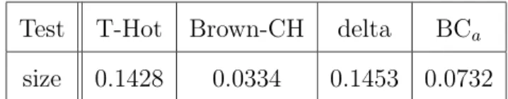
Test T-Hot Brown-CH delta BC

size 0.1428 0.0334 0.1453 0.0732 Table 2: Size of tests for (χ

− 1)/4 error

Figure 3: Size of the tests on the boundary of the hypotheses, where || θ || = 1 and

θ

> 0 for (χ

− 1)/4 error.

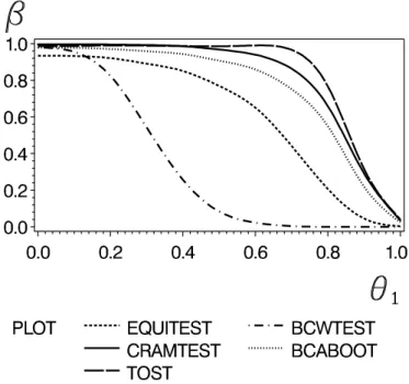
Figure 4: Power curves of the tests for n = 20, (χ

− 1)/4 error and 10.000 simulations.

The nominal level was α = 0.05.

In Figure 4 the resulting power functions are displayed. In summary we may draw the

following conclusions. The actual level is drastically exceeded by Munk & Pfl¨ uger’s

(1999) test as well as for the δ-method. Brown, Casella & Hwang’s (1995) method

performs rather accurate albeit very conservative for negative values of θ

. In contrast

the BC

method yields a very accurate approximation of the nominal level α = 0.05

over abroad range of θ

values. The differences in power between the two last named

tests are rather small. Note the the superior power of the other tests does not yield a

fair comparison due to its exceedance of the nominal level. In summary, only Brown,

Casella & Hwang’s (1995) method and the BC

-bootstrap are able to maintain the

given level under skewed errors. Interestingly, the power of the BCH test is significantly

increased by the χ

-error.

5 Examples

To demonstrate the practical relevance of the proposed methods we reanalyse the epilepsy data from the Introduction and an example of a multivariate bioavailability study from Chinchilli & Elswick (1997).

5.1 Example from neurology

In order to transfer the suggested methodology to the situation of Example 1 in the Introduction we require a generalization of Theorem 1 in Section 3 to the two sample case.

Theorem 2. Let X

, · · · , X

∼ F be an i.i.d. sample from a p-variate distribution F , and independently Y

, · · · , Y

∼ G an i.i.d. sample from a p-variate distribution G, s.t.

EX

− EY

= θ

− θ

= θ ∈ R

, Σ ˜

= Cov[X

], Σ ˜

= Cov[Y

] > 0 and E || X

||

, E || Y

||

<

∞ . Then we have for X = ¯ X − Y ¯ and Σ = (1+λ ˆ

) ˆ Σ

+(1+λ) ˆ Σ

with m/n → λ ∈ (0, ∞ ), that

T

:=

√ m + n(X

X − θ

θ) p 4X

ΣX ˆ

=

⇒ N (0, 1) for θ 6 = 0.

Proof. The proof is similar to Theorem 1, where we take into account that

√ m + n X ¯ − Y ¯ − θ =

⇒ (1 + λ

)

Z

+ (1 + λ)

Z

,

where Z

and Z

are independent p-variate normal r.v.s with covariances ˜ Σ

and ˜ Σ

, re-

spectively.

Observe, that for the case of equal covariances Σ

= Σ

(which we have assumed in this example) the asymptotic variance Σ = (λ + 1)

/λ Σ

. Observe further, that a BC

bootstrap test can be immediately obtained by drawing separately subsamples from the samples X

, · · · , X

and Y

, · · · , Y

.

In order to apply the afore mentioned equivalence tests we have to specify a bound ∆. Here we have chosen 20% of the range of the control group, for ESM and ESP , respectively.

Hence we end up with the testing problem

H :





1 4

θ

1 8

θ





2

2

> 1 versus K :





1 4

θ

1 8

θ





2

2

≤ 1 .

Test T-Hot Brown-CH delta BC

p-value 0.0101 0.0045 7.610

0.00989 Table 3: p-values for the epilepsy data

We mention that for the inversion of Hotelling’s confidence interval the pooled estimator

Σ = ˆ 1 n + m − 2

X

i=1,...,n

(X

− X) ¯

(X

− X) + ¯ X

j=1,...,m

(Y

− Y ¯ )

(Y

− Y ¯ )

!

has been used where the degrees of freedom of the F -distribution are now 2 and n + m − 2.

In summary we find that all tests decide significantly in favour of equivalence.

5.2 Bioequivalence study

The equivalence of availability of Ibuprofen in the blood of two drugs will be reinvestigated

for data presented by Chinchilli & Elswick (1997). Following these authors it is to be

tested whether the ratio of the expected AU C ’s (Area under the Curve) and the expected C max’s (maximal concentration) are between 0 .8 and 1.25.

In detail, it is assumed that independent bivariate r.v.’s are observed in a 2 × 2 crossover design without period effects. After a logarithmic transformation it is to assess whether

H

: | η

− η

| ≤ log 1.25 and | η

− η

| ≤ log 1.25 (9)

where η

and η

denotes the corresponding expectation of log AU C

and log C max.

Taking

X

:= 1

log 1.25 (log AU C

− log AU C

) , X

:= 1

log 1.25 (log C max

− log C max

)

yields the model from Theorem 1 with p = 2. After dividing the logarithms of raw data by

in order to transform the problem into the standardized form of the hypothesis in (3) we obtain the following summary statistics

(Mean difference) ¯ X =





− 0.121332 0.190746



, (Covariance) ˆ Σ =





0.1300518 0.1368549 0.1368549 0.8743755



 . For the complete data see Chinchilli & Elswick (1997). In our previous notation, we have θ = (

,

). In Table 2 we display the resulting p-values for the hypoth- esis (3). We find that all tests under consideration lead to a significant rejection of H, showing bivariate bioequivalence of the two ibuprofen formulations. Note, however, that the ordering of the p-values nicely reflects the superior power as found in the last section of the tests based on quadratic forms compared to the inclusion rules.

Test T-Hot BCH delta BC

p-value 0.00050 0.00021 ≤ 10

9.97710

Table 4: p-values for the Ibuprofen data.

6 Further Remarks and Extensions

Remark 3. Some readers may find it unsuitable for many purposes to choose ellipsoidal hypotheses instead of the more common rectangular ones. Nevertheless, we would like to mention, that even for the case of testing a hyperrectangle as in (9) our tests for ellipsoidal alternatives could be used. To this end, the largest sphere within the rectangle has to be chosen as the alternative (cf. again Figure 0). Throughout the following we have always chosen ∆ = 1 and p = 2.

In the following we investigate briefly how the ellipsoidal tests behave in comparison to the intersection union methods if they are used for rectangular hypotheses. Here, the intersection-union-test (TOST-test) has rejection region

p

\

i=1







| X

| < ∆

− t

s Σ ˆ

α







where X

denotes the i-th coordinate of X and t

the 1 − α quantile of a t-distribution with d degrees of freedom.

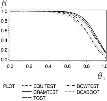
In Figure 5 the power curves of all tests are displayed under normal error assumption.

As it was expected the IU-test TOST is most powerful due to its property to be exactly

designed for a rectangular hypotheses. Note, that the BCH-test is significantly inferior

with respect to power whereas all the other tests have reasonable power.

Figure 5: Power curves of the tost procedure (TOST), δ-method (CRAMTEST), Munk

& Pfl¨ uger’s (1999) test (EQUITEST), the Brown et al. (1995) test (BCWTEST), and the BCA bootstrap (BCABOOT) for n = 20, normal error and 10.000 simulations. The

nominal level was α = 0.05.

Figure 6: Size of the tests on the boundary of the hypotheses, where θ

= 1 for normal error.

Figure 7: Power curves of the tests for n = 20, (χ

− 1)/4 error and 10.000 simulations.

The nominal level was α = 0.05.

In Figure 6 the nominal level is investigated where θ

∈ [ − 1, 1] and θ

= 1. It can be seen that again the BC

-test keeps the nominal level albeit rather conservative. The IU- method has size close to α = 0.05 over the entire range of θ

values besides those values of the hypothesis where θ

is close to -1 or 1.

In Figure 7 and Table 5 a similar scenario is investigated for skewed error. Observe, that

from Table 5 it follows that the IU-method now exceeds the nominal level whereas the

BC

method again keeps the nominal level rather accurate.

Test TOST T-Hot Brown-CH delta BC

size 0.1330 0.1390 0.0379 0.1516 0.0702 Table 5: Size of tests for (χ

− 1)/4 error

We mention that further simulations have shown (not displayed) that for increasing di- mension p the difference in power between both tests becomes smaller. When p = 10, the power of the BC

test is nearly the same as for the IU-method.

Remark 4. In practical applications often it is important to determine the required sam- ple size to achieve a preassigned power of the asymptotic tests for ellipsoidal hypotheses.

We will assume that X

, · · · , X

are independently normally distributed with expectation θ and covariance matrix ˜ Σ. The most interesting case occurs if exact equivalence holds, i.e. where θ = 0. In this case the power of the test ψ

(and hence asymptotically also of its BC

bootstrap version) is given as

P

√

n || X ||

− 1 2 p

X

ΣX ˆ

< u

!

= P

n || X ||

< n

u

2 p

X

ΣX ˆ + n .

Observe, that n || X ||

is distributed as P

j=1

˜ λ

U

where ˜ λ

are the eigenvalues of ˜ Σ and U

are i.i.d. standard normal r.v.’s. This is asymptotically a nondegenerate law whereas the r.h.s. expression n

u

2 p

X

ΣX ˆ = 2u

q

(n

X)

Σ(n ˆ

X) is asymptotically distributed as the square root of P

j=1

ζ

U

with ζ

being the eigenvalues of ˜ Σ

and the same r.v.’s

U

as before. The resulting law is rather complicated and hence we suggest to simulate

the resulting power for given ˜ Σ in order to obtain the required sample size. The case of

independent components is particularly simple and we give in Table 6 some values of the

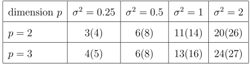
required sample size in order to achieve a power of 0.8 and 0.9, respectively.

dimension p σ

= 0.25 σ

= 0.5 σ

= 1 σ

= 2

p = 2 3(4) 6(8) 11(14) 20(26)

p = 3 4(5) 6(8) 13(16) 24(27)

Table 6: BC

-Bootstrap simulated sample sizes to achieve 0.8 (0.9) power for perfect equivalence θ = 0 for two and three dimensions for various variances of the independent

univariate normal variables (300 bootstrap replications)

We mention finally, that the above formula can be generalized of course to the two sample case, as treated in Theorem 4.2.

7 Conclusions

We have compared several tests for ellipsoidal hypothesis H : θ

Aθ ≥ ∆ versus K : θ

Aθ ≤

∆. It was shown that the BC

-bootstrap version of the test based on the statistic X

AX yields satisfactory results with respect to power and size. Even when this test is applied to rectangular hypotheses its power comes close to the intersection union test (which is only applicable for rectangular hypotheses), particularly as the dimension p of the parameter θ increases. Moreover, the suggested BC

bootstrap test is very robust against violation of the normality assumption of the error.

Finally we have proved asymptotic normality of the test statistic X

AX and the validity of the bootstrap principle for testing multivariate equivalence. This gives a theoretical justification for recent approaches suggested for dissolution profile testing where a similar test statistic was suggested and numerically investigated.

Acknowledgements

The author is indebted to A. Munk for raising the general question and constant guid-

ance in the analysis. R. Berger and G. Freitag pointed out some references. The financial

support of the Deutsche Forschungsgemeinschaft (SFB 475, ”Reduction of complexity in multivariate data structures”) is gratefully acknowledged.

References

– Aitchinson, J.: Confidence-region tests, Journ. Roy. Statist. Soc. B, 26 , 1964,

462-476. – Anderson, T.W.: An Introduction to Multivariate Statistical Analysis, John Wiley

& Sons, 1984, second edition.

– Berger, R.L.: Multiparameter hypothesis testing and acceptance sampling, Technometrics, 24 , 1982, 295-300.

– Berger, R.L., Hsu, J.C.: Bioequivalence trials, intersection-union tests, and equivalence confidence sets (with discussion), Statistical Science, 11 , 1996, 283-319.

– Box, G. E. P.: Some theorems on quadratic forms applied in the study of analysis of variance problems, I. effect of inequality of variance in the one-way classification. Ann. Math. Stat., 25 , 1954 290–302.

– Brown, L.D., Casella, G., Hwang, J.T.G.: Optimal confidence sets, bioequivalence, and the lima¸con of Pascal, Journ. Americ. Statist. Assoc., 90 , 1995, 880-889.

– Chinchilli, V.M., Elswick, R.K.jr.: The multivariate assessment of bioequivalence, Journ. Biopharmac. Statist., 7 , 1997, 113-123.

– Chow, S.-C., Liu, J.-P.: Design and Analysis of Bioavailability and Bioequivalence Studies, Marcel Dekker, 1992.

– Chow, Y.S., Teicher,H.: Probability Theory: Independence, Interchangeability, Martin- gales. 3rd ed. Springer Texts in Statistics. New York, NY: Springer, 1997.

– DasGupta, A., Gosh, J.K., Zen, M.M., A new general method for constructing confidence sets in arbitrary dimensions: with applications. Ann. Stat. 23 , 1995, 1408-1432.

– Dixon, P.M.: Assessing effect and no effect with equivalence tests. Risk Assessment: Logic and Measurement, eds. M. Newman & C. Strojan., Chelsea, MI: Ann Arbor Press., 1998.

– Efron, B., Tibshirani, R.J.: An Introduction to the Bootstrap, Chapman & Hall, 1993.

– Erickson, W.P., McDonald, L.L., Tests for bioequivalence of control media and test me- dia in studies if toxicity. Environ. Toxic. Chem. 14 , 1995, 1247-1256.

– United States Food and Drug Administration (FDA) Guidance for Industry: Disso- lution Testing of Immediate Release Solid Oral Disage Forms, U.S. Department of Health and Human Services, CDER, 1997.

– United States Food and Drug Administration (FDA): Bioavailability and bioequiv- alence requirements, U.S. Government Printing Office, 1992, U.S. Code of Federal Reglations, volume 21, chapter 320.

– Hauck, W.W., Anderson, S.: Types of bioequivalence and related statistical considera- tions. Intern. Journ. Clinic. Pharmacol., Ther. Toxic. 30 , 1992, 181-187.

– Hsu, H.C., Lu, H.L., Chan, K.K.H.: A novel multivariate approach for estimating the degree of similarity in bioavailability between two pharmaceutical products, Journ. Biopharma- ceutic. Statist., 84 , 1995, 768-772.

– Hwang, J.T.G. Comment on “Bioequivalence trials, intersection union tests and equivalence confidence sets”. Statistical Science, 11 , 1996, 313-315.

– Johnson, L.J., Kotz, S.: Continuous Univariate Distributions II, Houghton Mifflin Com- pany, 1969.

– Ma, M.-C. and Wang, B. B. C. and Liu, J.-P. and Tsong, Y., Assessment of similarity between dissolution profile. J. Biopharmaceut. Statist., 10 , 2000, 229-249.

– Mathai, A.M., Provost, S.B.: Quadratic Forms in Random Variables, Marcel Dekker, 1992.

– McBride, G.: Equivalence tests can enhance environmental statistics and managment, Aus- tral. New Zealand Journ. Statist., 41 , 1999, 19-29.

– Moore, J.W., Flanner, H.H.. Mathematical comparison of dissolution profiles. Pharma- ceut. Technology 20 , 1996, 64-74.

– Munk. A.: Correspondence: On a method of combining double t-test and Anderson-Hauck test, Biometrics, 50 , 1994, 884-886.

– Munk. A., Pfl¨ uger, R.: 1

− α equivariant confidence rules for convex alternatives are

2

- level tests – with applications to the multivariate assessment of bioequivalence, Journ. Americ.

Statist. Assoc., 94 , 1999, 1311-1320.

– Nakashima, K., Takahashi, K., Azumi, T., Ishida, G.: Exteroceptive suppression of the masseter and temporalis muscules produced by electric stimulation of the mental nerve in patients with Parkinson’s disease, Acta Neuro. Scand., 81 , 1990, 407-410.

– O’Hara, T., Dunne, A., Kinahan, A., Cunningham, S., Strak, P., Devane, J..

Review of methodologies for the comparison of dissolution profile data. IN: In vitro in Vivo Correlations, 1997, 167-171. Plenum Press, NY. Editors: Young et al.

– Roy, T., Calibrated nonparametric confidence sets, Journ. Mathem. Chemistry 21 , 1996, 103-109.

– Schall, R.: Assessment of individual and population bioequivalence using the probability that bioavailabilities are similar, Biometrics, 51 , 1995, 615-626.

– Schall, R., Groenewald, P.C.N., Potgieter, L.A., Luus, H.G.: Multivariate assess- ment of bioequivalence, Technical Report, University of the Orange Free State, 1996.

– Schoenen, J.: Exteroceptive suppression of temporalis muscle activity: methodological and physiological aspects, Cephalia, 13 , 1993, 3-10.

– Serfling, R., Approximation Theorems of Mathematical Statistics, Wiley, 1980.

– Shah, V. P. and Tsong, Y. and Sathe, P. and Liu, J.-P., In vitro dissolution profile comparison - statistics and analysis of the similarity factor, f

, Pharmres, 15 , 1998, 889–896.

– Sierra-Cavazos, J.H., Berger, R.L. Intersection-union tests in dissolution profile testing.

Technical Report, NCSU Institute of Statistics Mimeo ser. No. 2521, 1999.

– Steinhoff, B.J., Fangmeier, B., Reimers, C.D., Paulus, W.: Einfluß von Epilepsien und antiseptischer Medikation auf die exterozeptive Suppression der Temporalismuskelaktivit¨at, Zeitschrift f¨ ur Elektroenzephalographie, Elektromyographie und verwandte Gebiete, 2 , 1996, 65- 69.

– Wang, W., DasGupta, A., Hwang, J.T.G.: Statistical tests for multivariate bioequiva-

lence, Biometrika 86 , 1999, 395-402.