Testing for symmetries in multivariate inverse problems

SFB 823

Testing for symmetries in

multivariate inverse problems

Discussion Paper

Melanie Birke, Nicolai Bissantz

Nr. 17/2011

Testing for symmetries in multivariate inverse problems

Melanie Birke

Ruhr-Universit¨ at Bochum Fakult¨ at f¨ ur Mathematik 44780 Bochum, Germany

e-mail: melanie.birke@rub.de

Nicolai Bissantz Ruhr-Universit¨ at Bochum

Fakult¨ at f¨ ur Mathematik 44780 Bochum, Germany

e-mail: nicolai.bissantz@rub.de

April 19, 2011

Abstract

We propose a test for shape constraints which can be expressed by transformations of the coordinates of multivariate regression functions. The method is motivated by the constraint of symmetry with respect to some unknown hyperplane but can easily be generalized to other shape constraints of this type or other semi-parametric settings. In a first step, the unknown parameters are estimated and in a second step, this estimator is used in the L₂-type test statistic for the shape constraint. We consider the asymptotic behavior of the estimated parameter and show, that it converges with parametric rate if the shape constraint is true.

Moreover we derive the asymptotic distribution of the test statistic under the null hypothesis and furthermore propose a bootstrap test based on the residual bootstrap. In a simulation study we investigate the finite sample performance of the estimator as well as the bootstrap test.

Keywords: Deconvolution, Goodness-of-Fit, Inverse Problems, Semi-Parametric Regression, Sym- metry

1 Introduction

Several kinds of symmetry play an important role in many areas of research. For example, many objects or parts of objects are symmetric with respect to reflection or rotation. Symmetry can be used in image compression and also in image analysis to detect certain objects. If symmetry of a certain object is violated one can sometimes deduce some results from it. Usually, parts of the human body are (nearly) symmetric, e.g. the left hand is symmetric to the right hand, the left part of the face to the right part and so on. This is usually also true for the thermographic distribution of those parts. If in a thermographic image of both hands this symmetry is severely violated, this can be a hint to some inflammation in this part. Problems of this and similar type make testing for symmetry to a problem of considerable interest. Technically, modeling the object of interest

as a multivariate function, we end up with the problem of testing for symmetry of a multivariate function.

Whereas several results exist which discuss the symmetry of density functions (see e.g. Ahmad and Li (1997), Caba˜na and Caba˜na (2000) and Dette, Kusi-Appiah and Neumeyer (2002) among many others) only few authors have considered testing for symmetry of a regression function so far.

Recent results have been presented in Bissantz, Holzmann and Pawlak (2009) and Birke, Dette and Stahljans (2011), where both are for the case of bivariate functions in direkt regression models and for symmetry with respect to some known axis.

In some cases it is not possible to observe the object of interest directly. This leads to an inverse problem. Testing for symmetry in inverse regression problems can be of even higher interest than testing for symmetry in direct regression models. The reason is as follows. Whereas, at least in bivariate settings, symmetry in direct regression models can approximately be recognized by simply looking at the data, symmetrical structures in the true object can lack any symmetry in the observed (indirect) data. Consider, for example, the well known convolution problem which commonly appears in image analysis where the true object is distorted by a so called point-spread function we can easily find situations (e.g. for asymmetric point-spread functions or if the point- spread function has a different axis of symmetry than the true object) where the symmetry is not visible in the image. To the best of our knowledge there are no methods for testing for symmetry in inverse regression problems so far.

In the following we will develop a testing procedure for reflection symmetry of d-variate functions with respect to some hyperplane of dimensiond−1. The method can, however, easily be generalized to rotational symmetry or other shape constraints of similar type. Therefore, whereas we motivate the problem by the case of a symmetry constraint, the theoretical results and their proofs will be formulated as general as possible. Since the symmetry hyperplane is unknown we estimate it in a first step by minimizing an L2-criterion function. If the true function is really symmetric with respect to this hyperplane, we derive, under some regularity conditions, consistency with parametric rate of the estimator and show that it is asymptotically normally distributed. In a second step, we use the minimized criterion function as test statistic for symmetry and show that it is asymptotically normal. Since the problem under consideration is closely related to certain semi- parametric problems we will use similar techniques as H¨ardle and Marron (1990). However note the important differences, that our problem is inverse and our regression function is multivariate.

In nonparametric regression tests based on such asymptotic distributions usually do not perform satisfactorily in finite samples because the convergence is very slow and there is the problem of dealing with a bias term. To avoid this problem we propose a bootstrap test based on residual bootstrap and investigate the finite sample performance of this test in a simulation study.

The rest of the paper is organized as follows. In section 2 we describe the model and define the estimator for the hyperplane as well as the test statistic. The asymptotic behavior of both is considered in section 3 while we show the finite sample performance in section 4. Finally all proofs are defered to the appendix

2 The model and test statistic

We consider the nonparametric inverse regression model

Y_r= Ψm(x_r) +σε_r (1)

with x_r= (r₁/(n₁a_n1), . . . , r_d/(n_da_nd))^T, r_j =−n_j, . . . , n_j and a_nj →0,j = 1, . . . , d such that with increasing sample size we have observations on the wholeR^d. For the sake of simplicity we assume in the following that n_j = n and a_nj = a_n such that x_r = (r₁, . . . , r_d)^T/(na_n) and for fixed n we have observations on the compact set I_n = [−1/a_n,1/a_n]^d. In (1) m is a two times continuously differentiable regression function, and Ψ is an operator which maps m to the convolution m ∗ψ with a known convolution functionψ. Finally, withr= (r₁, . . . , r_d),{ε_r}ⁿr∈{−n...,n}^d are independent identically distributed errors with E[ε_r] = 0, E[ε²_r] = 1 and E[ε⁴_r]<∞. If m isj times continuously differentiable according to Bissantz and Birke (2009)

ˆ

m^(j)(x) = X

r∈{−n,...,n}^d

wr,j(x)Yr (2)

with

w_r,j(x) = 1

(2π)^d/2(nh^ja_n)^d Z

[−1,1]^d

(−iω)^je^{−iωT(x−xr)/h}

Φ_ψ(ω/h) dω (3)

with j = (j₁, . . . , j_d), j =j₁ +. . .+j_d is an appropriate estimate for ^∂j1+...+jd

∂x^j₁¹...∂x^jd_d m. If j = 0 we write ˆ

m⁽⁰⁾(x) = ˆm(x) and w_r,0(x) =w_r(x). As an abbreviation we write in the following Ψm =g. In (3) Φ_f denotes the Fourier transform of a functionf.

We consider the case of reflection symmetry with respect to some hyperplane in R^d parameterized by θ ∈ R^d. Then, for every fixed θ ∈ R^d mirrowing m at the corresponding hyperplane can be realized by some linear functional T_θS_θ⁻¹ where T_θ contains the shift of the hyperplane and the rotation and S_θ⁻¹ is mainly the inverse of T_θ concatenated with the mirrowing at the (x₂, . . . , x_d)- hyperplane }_θ. The condition of symmetry of m with respect to that hyperplane in some areaA_θ around that hyperplane is

m(z) =m(T_θS_θ⁻¹z) for all z∈A_θ (4) or equivalently

m(Tθx) =m(Sθx) for all x∈A =T_θ⁻¹Aθ. (5) To this end we will use

L(θ) = Z

A

(m(T_θx)−m(S_θx))²dx. (6)

to check whethermexhibits such a symmetry onA_θ. In the following we will assume without loss of generality thatA =T_θ⁻¹A_θ is independent ofθ. The parameterϑ of the true hyperplane minimizes this criterion function. Since m is not known, we estimate the criterion function as

Lˆ_n(θ) = Z

A

( ˆm(T_θx)−m(Sˆ _θx))²dx (7)

and find the estimator of ϑ by minimizing ˆLn(θ) ϑˆ = arg min

θ∈B0×B1

Lˆ_n(θ),

where B₀ ⊂R^d−1 is the compact set of all possible rotation angles and B₁ ⊂R the compact set of all possible shifts. If ˆm is continuously differentiable, we can equivalently solve

ˆl_n(θ) = grad ˆL_n(θ) = 0 (8)

to find ˆϑ.

Example. For illustrational purposes we discuss the case d = 2. Here, the hyperplane reduces to a straight line parameterized by }_θ = n

(cosθ₁,sinθ₁)^T λ+θ₂(−sin(θ₁),cos(θ₁))^T |λ∈R o

, θ = (θ₁, θ₂)^T ∈ R² unknown such that mirrowing z ∈ R² at that straight line can be obtained by transforming z to

T_θ⁻¹z= cosθ₁ sinθ₁

−sinθ₁ cosθ₁

!

z− 0 θ₂

! ,

mirrowing at }₀ =n

(0,1)^T λ|λ∈R o

which gives

S_θ⁻¹z= −1 0 0 1

! T_θ⁻¹z

and transforming back, which finally yields

TθS_θ⁻¹z.

3 Asymptotic inference

To consider asymptotic theory, we further assume that Ψ is ordinary smooth, i.e. we consider mildly ill-posed problems in model (1). This can be summarized in the following assumption.

Assumption 1. The Fourier transform Φ_ψ satisfies

|Φ_ψ(ω)| |ω|^β →κ, ω → ∞ for some β >0 and κ∈R\ {0}.

Assumption 2. The Fourier transform Φ_m ofmsatisfiesR

R|Φ_m(ω)||ω|^kdω <∞for any multiindex k with k₁+. . .+k_d≤r for some r > β+ 1 andm is two times continuously differentiable

Assumption 3. The bandwidth h fulfills h → 0, n^d/2a^d/2n h^β+d → ∞, (logn)^1/4/n^dh^da^d_n = o(1), n^dh2β+2s+d/2−1a^3d/2n →0 and a^r_n=o(h^β+s+d−1)

Assumption 2 is, for example fulfilled, if for grad (m) (and hence also for the products and sums in the integral) the k-th derivative exists for all ||k|| ≤β. Note also, that in Assumption 3 a_n cannot be seen as regularization parameter since it is determined by the underlying design. Therefore, all conditions have to be read as conditions on hn, s, β, j and r dependent on the rate of an.

Under the above conditions we can now discuss the asymptotic properties. We first consider the consistency and the asymptotic distribution of the estimator ˆϑ

Theorem 1. Let L(θ) be locally convex near the true parameter ϑ. Then, under Assumptions 1 ϑˆ_n →^P ϑ for n → ∞.

Theorem 2. If mˆ is continuously differentiable, ϑˆ is defined by (8) and }_ϑ is the true symmetry hyperplane, we have

pn^da^d_n

ϑˆ−ϑ _D

→ N(0, σ²h⁻¹(ϑ)Σ(ϑ)(h⁻¹(ϑ))^T) with

Σ(θ) = σ² (2π²κ)^d

Z

R^d

Z

R^d

||ω||^βI_[−1,1]^d(ω)e^−iωTydydω

2Z

R^d

σθ(u)σθ(u)^Tdu σθ(u) =

∂

∂θTθ

(T_θ⁻¹(u))−MθN_θ⁻¹ ∂

∂θSθ

(T_θ⁻¹(u))−NθM_θ⁻¹ ∂

∂θTθ

(S_θ⁻¹(u))

− ∂

∂θS_θ

(S_θ⁻¹(u)) T

(grad m(u))^T h(θ) = 2

Z

A

grad m(Tθx) ∂

∂θTθx−grad m(Sθx) ∂

∂θSθx grad m(Tθx) ∂

∂θTθx−grad m(Sθx) ∂

∂θSθx T

dx The second point of interest is to test whether the image obeys a symmetry of some kind. We use

the test statistic

Lˆ_n( ˆϑ) = Z

A

( ˆm(Tϑˆx)−m(Sˆ ϑˆx))²dx (9) which has the following asymptotic distribution.

Theorem 3. Under the above assumptions, if ϑ parametrizes the true symmetry hyperplane, we have

σ^−1/2_n Lˆ_n( ˆϑ)− 2σ² (2π)^dn^dh^2β+da^d_n

Z

A

Z

[−1,1]^d

|ω|^2β

sin

ω^TS_ϑx h

2

dωdx

!

→ ND (0,1) with

σ_n= 32σ⁴

κ⁴(2π)^2dn^2dh^2d+4βa^2d_n Z

R^2d

|ω|^2β|η|^2β

Z

A

sin

ω^TSϑx h

sin

η^TSϑx h

dx

2

d(ω, η)

It can be shown similarly as in the proof of Theorem 4 in the Appendix, that the effective rate of convergence is n^dh^2β+d/2a^3d/2n .

4 Simulations

4.1 Simulation framework

In this section we present the results of a simulation study. To this end we generate observations according to model (1), i.e.

Y_(r,s) = Ψm(x_(r,s)) +σε_(r,s).

In our simulations, the noise terms are i.i.d. normally distributed with variance 1 andx_(r,s)= _n^r,_n^s , (r, s) ∈ {−n,−n+ 1, . . . , n−1, n}² are the coordinates of a grid with equidistant stepsize in both coordinates and with a_n = 1. In the following we use the parameter values n = 50 and σ (in dependence of the underlying function m) such that σ makes up for 1/10-th and 1/25-th of the maximum of the signal Ψm, which amounts to signal-to-noise ratios - defined as the mean signal of the image divided byσ - of ≈10 and ≈4, respectively. These values amount to rather poor signal- to-noise ratios, and in a practical application,S/N will frequently be larger and our simulations be expected to be conservative with respect to the performance of our method.

We consider two different ”true” imagesm₁ andm₂ from which the data is generated. These images represent the cases of having a unique axis of symmetry (image m1) and of not having any axis of symmetry at all (image m₂). The images are generated from the following bivariate functions (with (x_t, y_t)∈R²).

m₁(x, y) = exp(−3·(4·x²_t + (y_t+ 0.1)²)) + 0.5·exp(−3·(x²_t + 3·(y_t−0.4)²)) m₂(x, y) = 0.5·exp(−5·((x_t−0.3)²+ 5·(y_t+ 0.3)²+))

+ 0.5·exp(−5·((xt+ 0.2)²+ 5·(yt−0.3)²)) + 0.5·exp(−5·((xt+ 0.5)²+ 5·(yt+ 0.6)²)), where

x_t y_t

!

= cos(α) −sin(α) sin(α) cos(α)

! x y

!

+ −δ

0

!

are the coordinates of a coordinate system which is rotated by an angle α= −0.3 with respect to the original coordinate system ofy in counterclockwise direction and shifted (along the transformed y_t-axis) by δ = 0.1. Hence, image m₁ is symmetric with respect to an axis of symmetry which passes thex-axis at x= 0.1 and is tilted away to the right from they-axis by an angle of−0.3 rad., that is ϑ= (α, δ)^T = (−0.3,0.1)^T

In accordance with model 1 for the observations, we do not assume to be able to observem_idirectly, but that at our disposal are only observations of the convolution of m_i,i= 1,2 with a convolution function ψ given by

ψ(x, y) = λ 2 ·exp

−λ·p

x²+ 0.25·y²

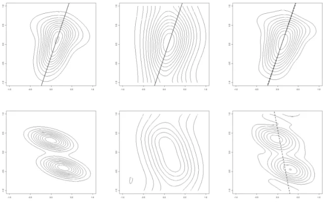
(with λ = 5). Figure 1 shows the images of m₁ and m₂, their convolutions with Ψ and typical examples for estimates ˆm1 and ˆm2.

The convolution functionψis symmetric with respect to thex- andy-axis of the (original) coordinate system, that is symmetric with respect to axes which are different to the axes of symmetry ofm₁. In consequence, the convolved (observed) image Ψm1 does not have any axis of axial symmetry. Note

Figure 1: True images and typical examples for the observed image and associated selected axis for m₁ (top panels)andm₂ (bottom panels). Left column: true functions, middle column: true function convolved with Ψ, right column: reconstructions from data with n = 50, S/N = 25. The full line indicates the true axis of symmetry and the dashed line the estimated symmetry axis. Note that m₂ is not symmetric to any axis, hence the full line is missing.

that this implies that testing for symmetry of m can in general not be substituted by testing for symmetry of Ψm, except under specific, strong assumptions on the symmetry properties of m and ψ. Instead, it is required that the observed image is deconvolved in a first step, with the symmetry test being performed in a subsequent second step.

In our simulations we use the spectral cut-off estimator (2) with equal bandwidths in both coordinate axes. From a visual inspection of 5 randomly selected noisy images and the associated estimates ˆm we chose h≈0.05. This bandwidth was kept fixed in all subsequent simulations.

4.2 Critical functions and the distribution of estimated parameters and test statistics

In this section we describe the performance of the estimators for the symmetry axis parameters δ andα, and the properties of the underlying criterion function (7), which can, as already pointed out in Section 3, be used as test statistic for symmery of the regression function, for the two different images considered here.

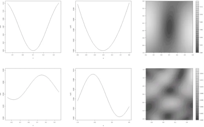
Figure 2: True (noiseless) criterion function Ln for the translation axis form1 (top panels) and m2

(bottom panels) for n = 50 and signal-to-noise ration S/N = 25. Left column: L_n(δ) forα =−0.3 assumed to be known, middle column: L_n(α) for δ = 0.1 assumed to be known, right column:

Ln(δ, α).

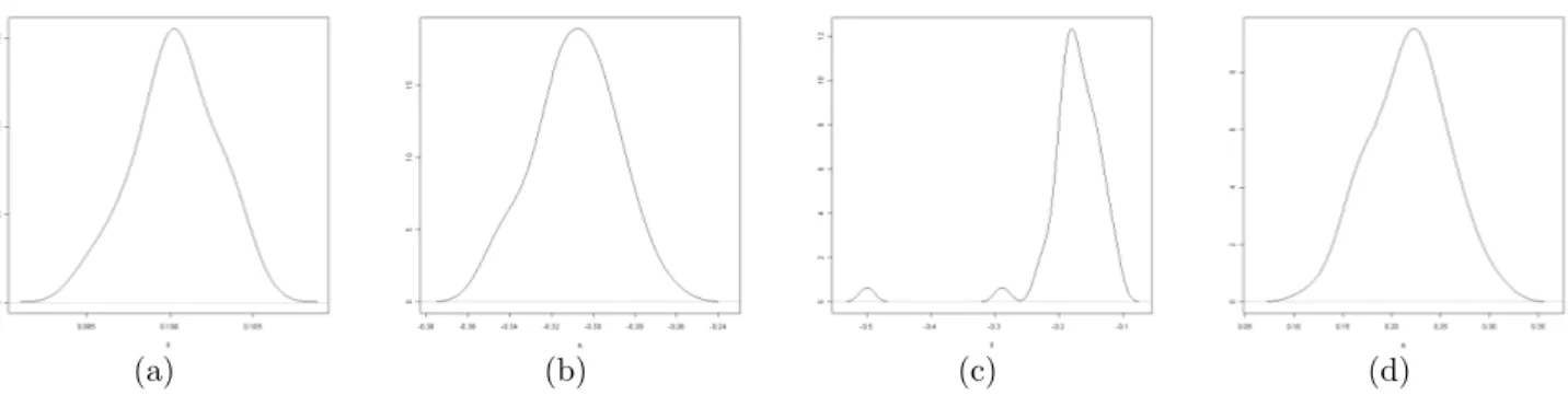
(a) (b) (c) (d)

Figure 3: Distribution of the estimated symmetry parameters form₁ ((a) and (c)) andm₂ ((b) and (d)). (a) and (b): only shift estimated, (c) and (d): only rotation angle estimated for sample size parameter n= 50, and signal-to-noise ratio S/N = 25.

Figure 2 shows the critical functionL_n(δ, α) both for the case of univariate estimation of the shiftδ resp. the angle α(where the other parameter is assumed to be known) and for bivariate estimation of the pair (δ, α). For m₂ the criterion function for the selection of the shift only (top right panel) does not come close to the minimal value it attains for the symmetric function m₁ at all, but the situation is different for the estimation of the rotation angle, where the minimal values differ less strongly. Now consider the bivariate estimation of shift and rotation angle. For m₂, a complicated pattern appears without a distinct minimum.

Next, Figure 3 shows the simulated distribution of the estimated parameters for rotation and shift for the various simulation setups. For m₂, which does not have an axis of symmetry at all, the critical function still showes clear minima of the criterion function if only one of the parameters was estimated. This is reflected in the right column of Figure 3 for the estimated parameter, that is the value where the minimum is attained.

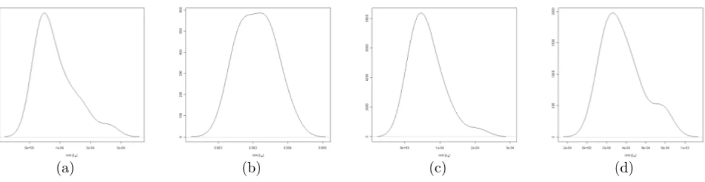
Finally, consider Figure 4, which compares the simulated distributions of the test statistic for the case of one parameter estimated under H₀ (i.e. for m₁) with the results under H₁ (i.e. for m₂). In the latter case the distributions are shifted to significantly larger mean values, which reflects the fact that there exists no axis of symmetry. Moreover, their shape appears more symmetric than underH₀, where it is (much) more skewed to the right, similar to otherL₂-based test statistics (e.g.

Dette (1999), Bissantz et al. (2010) and Birke, Dette and Stahljans (2011)).

4.3 Testing for symmetry

In the final part of our simulations let us now turn to a more precise analysis of the performance of our proposed test for symmetry. Since the convergence of L₂-tests is known to be slow and the asymptotic distribution apparently depends on unknown parameters we use bootstrap quantiles as critical values for the test.

Hence, our testing procedure consists of two main parts. In the first bootstrap part we determine a bootstrap approximation to the distribution of the test statistics. In more detail, this consists of three steps: (1) to estimate the distribution of residuals, (2) to determine a ”true image” ˆm_B from

(a) (b) (c) (d)

Figure 4: Distribution of the test statistics under H₀ : m = m₁ ((a) and (c)) resp. m = m₂ ((b) and (d)). (a) and (b): only shift estimated, (c) and (d): only rotation angle estimated for sample size parameter n = 50, and signal-to-noise ratio S/N = 25.

which the bootstrap data are generated, and (3) to perform the bootstrap replications of the test statistic. The subsequent, second test decision part of the procedure is performed by computation of the test statistic for the original (observed) data and a decision based on this test statistic and the bootstrap approximation to its distribution. We now describe all steps in detail.

A. Bootstrap part of the testing procedure:

1. Estimation of the distribution of residuals: In our simulations we use a residual bootstrap as follows. In the first step we determine the empirical distribution of the residuals as the cen- tered distribution of differences between the observations and an estimate Ψ ˆm of Ψm. Then, in each of the bootstrap replications, we draw residuals from this distribution and generate bootstrap data as the sum of a suitable ”true bootstrap image” ˆm_B and these residuals.

2. Determination of a ”true image” ˆm_B: The ”true bootstrap image” ˆm_B is generated as fol- lows such that it obeys a known axis of symmetry and closely resembles the true (unknown) function m, assuming H₀ to be true.

Step 2.1 - Estimating m: Determination of an estimate ˆm of m as described above.

Step 2.2 - Estimation of symmetry axis parameter: Minimization of the criterion func- tion yields estimates ˆδ and/or ˆα of the symmetry axis parameter(s) of ˆm.

Step 2.3 - Backshift and rotation of m:ˆ We shift and rotate ˆm back by the estimated parameters ˆδand/or ˆα(and, if applicable, the known true values of the other parameter).

UnderH₀, and if no noise would be present in the observed data, the new image ˇmwould now be symmetric with respect to they-axis.

Step 2.4 - Symmetrization: To ensure symmetry, we average the image over both sides of the y-axis, that is according to the scheme ˜m(x, y) = ¹₂( ˇm(x, y) + ˇm(−x, y)) for all (x, y).

Step 2.5 - Backrotation and -shifting of the image to the estimated symmetry axis:

The image ˜m is rotated and shifted such that it is symmetric with respect to the axis

S/N = 10 S/N = 25

Hypothesis/Nominal level 5% 10% 20% 5% 10% 20%

H₀ : m=m₁ 5.5% 10.5% 21.5% 6.5% 11.0% 20.5%

H₁, κ= 0.1 8.0% 12.0% 23.5% 8.5% 17.0% 27.0%

H₁, κ= 0.2 10.5% 20.0% 33.0% 54.0% 70.5% 81.5%

H₁, κ= 0.4 57.0% 71.5% 82.0% 100% 100% 100%

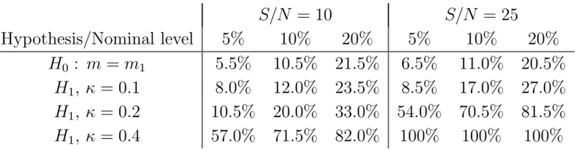
Table 1: Estimated rejection probabilities of the test for axial symmetry from 200 simulations each in case of estimating the axis-shiftδ(withα known), underH₀ : m=m₁, and under an alternative m=κ·m₂+ (1−κ)·m₁, respectively.

S/N = 10 S/N = 25 Hypothesis/Nominal level 5% 10% 20% 5% 10% 20%

H0 : m=m1 0% 2% 7% 6% 12% 20%

H₁, κ= 0.4 3% 5% 15% 8% 19% 39%

H₁, κ= 1.0 9% 19% 50% 78% 87% 96%

Table 2: Estimated rejection probabilities of the test for axial symmetry from 100 simulations each in case of estimating both the axis-shift δ and the angle of rotation α, and under an alternative m=κ·m2+ (1−κ)·m1, respectively.

with the estimated parameters ˆδ and/or ˆα, or - if applicable - the known values of shift and rotation, respectively. We call the resulting image ˆm_B.

3. Bootstrap replications: In the final step of the bootstrap part of the testing procedure we generate bootstrap data from the modelY_r^∗ = Ψ ˆmB(xr)+ε^∗_r, whereε^∗_rare drawn independently from the empirical distribution of the residuals ˆε_r =Y_r−Ψ ˆm(x_r). From each set of bootstrap data the image is estimated and the minimal value of the criterion function, that is the test statistics, determined. In our simulations we always use B = 200 bootstrap replications. The bB(1−α)c-th order statistic of all those bootstrap test statistics gives the critical value for the test.

Test decision part of the testing procedure:

In the second part of the testing procedure we use once more the estimate ˆm ofm described above.

From this estimate we determine the test statistics ˆL_n( ˆα,ˆδ), that is the minimal value of the cri- terion function (9). The test decision by itself is then to reject the null hypothesis of m obeying an axial symmetry to level α, if the test statistics for the original set of data is larger than the (1−α)-quantile of the bootstrap distribution of the test statistics.

In the following, we consider the functions

mκ(x, y) = κm2(x, y) + (1−κ)m1(x, y), κ= 0,0.1,0.2,0.4,1

to analyse the sensitivity of our test to small deviations from symmetry. Tables 1 and 2 summarize the simulated levels and power of the test for axial symmetry for the case of an unknown shift parameterδ only (withα known), and for the case that both parameters are unknown. The results demonstrate the substantial additional difficulty of disproving the existence ofanyaxis of symmetry if both δ and α are unknown. Slightly acceptable results for the moderate sample size of n = 50 only appear for a comparable large deviation from symmetry (i.e. κ = 1). This effect is to a large part due to the complicated shape of the critical function in this case (cf. Fig. 2) with several local minima. If only the shift parameter is unknown, the test already performes well for small devi- ations from symmetry (e.g. κ= 0.2 for a signal-to-noise ratio ofS/N = 25 orκ = 0.4 forS/N = 10).

Acknowledgements. This work has been supported in part by the Collaborative Research Center

”Statistical modeling of nonlinear dynamic processes” (SFB 823 project C4) of the German Research Foundation and the BMBF project INVERS.

References

I.A. Ahmad and Q. Li (1997). Testing symmetry of an unknown density function by kernel method.

Nonparam. Statist. 7, 279-293.

M. Birke, H. Dette, K. Stahljans (2011). Testing symmetry of a nonparametric bivariate regression function. Nonparam. Statist., to appear

N. Bissantz and M. Birke (2009). Asymptotic normality and confidence intervals for inverse regres- sion models with convolution-type operators. J. Multivariate Anal. 100, 2364 - 2375.

N. Bissantz, H. Dette, K. Proksch (2010). Model checks in inverse regression models with convolution- type operators. Technical report SFB 823.

Bissantz, Holzmann and Pawlak (2009). Testing for Image Symmetries - with Application to Con- focal Microscopy. IEEE Trans. Information Theory 55, 1841-1855.

A. Caba˜na and M. Caba˜na (2000). Tests of symmetry based on transformed empirical processes.

Canad. J. Statist. 28, 829-839.

H. Dette (1999). A consistent test for the functional form of a regression based on a difference of variance estimators. Ann. Statist. 27, 1012 - 1040.

H. Dette, S. Kusi-Appiah and N. Neumeyer (2002). Testing symmetry in nonparametric regression models. Nonparam. Statist. 14 (5), 477-494.

Eubank, R.L. (1999). Nonparametric regression and spline smoothing. Second edition. Statistics:

Textbooks and Monographs, 157. Marcel Dekker, Inc., New York

W. H¨ardle and J.S. Marron (1990). Semiparametric Comparison of Regression Curves. Ann.

Statist. 18, 63-89

P. de Jong (1987). A Central Limit Theorem for Generalized Quadratic Forms. Probab. Th. Rel.

Fields 75, 261-277

A Proofs

Theorem 4.

n^dh^2j+2β+d/2a^3d/2_n Z

B

mˆ^(j)(x)−m^(j)(x)²

dx− 2^dσ²Qd

k=1(2(j_k+β_k) + 1)⁻¹ κπ^dn^dh^2j+2β+da^2d_n

!

→ ND (0, s^(j))

for j= (j₁, . . . , j_k) with j₁+. . .+j_k ≤2 and s^(j) = 2σ⁴

κ²(2π)^2d lim

n→∞

d

Y

l=1

a_nh^4βl+4jl+1 Z Z

I[−1,1](ω_l)I[−1,1](η_l)|ω_lη_l|^2jl+2βlsin²(^ωl_a^−ηl

n )

(ω_l−η_l)² dω_ldη_l

Proof. In the following we write the L²-distance as a quadratic form and some bias terms and apply a central limit theorem by de Jong (1987). There is

Z

B

mˆ^(j)(x)−m^(j)(x)² dx =

Z

B

X

r

w_r,j(x)ε_r

!2

dx+ 2 Z

B

X

r

w_r,j(x)ε_r

!

(E[ ˆm^(j)(x)]−m^(j)(x))dx +

Z

B

(E[ ˆm^(j)(x)]−m^(j)(x))²dx

= I₁^(j)+I₂^(j)+I₃^(j).

Using the definition of wr,j(x) and Parseval’s equality we obtain I₁^(j) = 1

(2π)^dn^2dh^2j+da^2d_n Z

R^d

|ω|^2j I_[−1,1]^d(ω)

|Φ_ψ(ω/h)|²

X

r

e^iωTxr/hεr

2

dω

− 1

(2π)^dn^2dh^2j+da^2d_n Z

(B/h)^c

Z

R^d

e^−iωTx(−iω)^jI_[−1,1]^d(ω) Φψ(ω/h)

X

r

e^iωTxr/hε_rdω

2

dx

= I_1.1^(j)−I_1.2^(j). We write

I_1.1^(j) = X

u

a^(j)_u,uε˜²_u+ ˜ε^TA˜^(j)ε˜=I_1.1.1^(j) +I_1.1.2^(j) with

a^(j)_u,v = 1

(2π)^dn^2dh^2j+da^2d_n Z

R^d

|ω|^2j I_[−1,1]^d(ω)

|Φ_ψ(ω/h)|²e^iωTx˜u/he^{−iωT˜xv/h}dω A˜^(j) = (˜a^(j)_u,v)1≤u,v≤(2n+1)^d, ˜a^(j)_u,v =a^(j)_u,v for u6=v, ˜a^(j)_u,u = 0

˜

x₁ = x(−n,...,−n), . . . ,x˜_(2n+1)d =x_(n,...,n)

˜

ε^T = (˜ε1, . . . ,ε˜_(2n+1)^d) = (ε(−n,...,−n), . . . , ε_(n,...,n))∈R⁽²ⁿ⁺¹⁾

d.

For I_1.1.1^(j) we obtain E[I_1.1.1^(j) ] = σ²X

u

a^(j)_u,u = σ²

(2π)^dn^2dh^2j+da^2d_n X

r

Z

R^d

|ω|^2j I_[−1,1]^d(ω)

|Φ_ψ(ω/h)|²dω

= σ²(2n+ 1)^d (2π)^dn^2dh^2j+da^2d_n

Z

R^d

|ω|^2j I_[−1,1]d(ω)

|Φ_ψ(ω/h)|²dω

∼ σ²(2n+ 1)^d κ²(2π)^dn^2dh^2j+2β+da^2d_n

Z

R^d

|ω|^2j+2βI_[−1,1]^d(ω)dω

= σ²(2n+ 1)^d κ²π^dn^2dh^2j+2β+da^2d_n

d

Y

k=1

1

2(jk+βk) + 1 =O

1 n^dh^2j+2β+da^2d_n

Var(I_1.1.1) = X

u

a^(j)_u,u2

µ₄(ε) = µ₄(ε) (2π)^2dn^4dh^4j+2da^4d_n

X

r

Z

R^d

|ω|^2j I_[−1,1]^d(ω)

|Φ_ψ(ω/h)|²dω 2

= µ₄(ε)(2n+ 1)^d (2π)^2dn^4dh^4j+2da^4d_n

Z

R^d

|ω|^2j I_[−1,1]^d(ω)

|Φψ(ω/h)|^{2 2}

dω

∼ µ₄(ε)(2n+ 1)^d κ⁴(2π)^2dn^4dh^4j+4β+2da^4d_n

Z

R^d

|ω|^2j+2β|I[−1,1]^d(ω)|²dω 2

=O

1

n^3dh^4j+4β+2da^4d_n

= o

1 n^2dh^4j+4β+da^3d_n

.

We now check the assumptions of Theorem 5.2 in de Jong (1987) for I_1.1.2. First of all we calculate the variance

σ(n)² = Var(˜ε^TA˜^(j)ε) = 2σ˜ ⁴tr( ˜A^(j))² = 2σ⁴X

u6=v

(a^(j)_u,v)²

= 2σ⁴

(2π)^2dn^4dh^4j+2da^4d_n X

r6=s

Z

R^d

|ω|^2j I_[−1,1]d(ω)

|Φ_ψ(ω/h)|²e^iωTxr/he^−iωTxs/hdω 2

∼ 2σ⁴ (2π)^2dn^2dh^4ja^2d_n

Z

In/h

Z

In/h

Z

R^d

|ω|^2j I[−1,1]^d(ω)

|Φ_ψ(ω/h)|²e^iωTy/he^−iωTz/hdω 2

dydz

= 2σ⁴

(2π)^2dn^2dh^4ja^2d_n Z

R^d

Z

R^d

|ω|^2j|η|^2j I_[−1,1]^d(ω)I_[−1,1]^d(η)

|Φ_ψ(ω/h)|²|Φ_ψ(η/h)|² Z

In/h

e^i(ω−η)Tudu

2

dωdη

= 2σ⁴

(2π)^2dn^2dh^4ja^2d_n Z

R^d

Z

R^d

|ω|^2j|η|^2j I_[−1,1]d(ω)I_[−1,1]d(η)

|Φ_ψ(ω/h)|²|Φ_ψ(η/h)|²

d

Y

l=1

|e^{i(ωl−ηl)/(han)}−e^{−i(ωl−ηl)/(han)}|²

|ω_l−η_l|² dωdη

= 2σ⁴

κ⁴(2π)^2dn^2dh^4j+4βa^2d_n Z

R^d

Z

R^d

I_[−1,1]^d(ω)I_[−1,1]^d(η)

d

Y

l=1

|ω_l|^2jl+2βl|η_l|^2jl+2βl|sin(^ω_ha^l−ηl

n )|²

|ωl−ηl|² dωdη

= 2σ⁴

κ⁴(2π)^2dn^2dh^4j+4βa^2d_n

d

Y

l=1

Z

R

Z

R

I[−1,1](ωl)I[−1,1](ηl)|ωlηl|^2jl+2βlsin²(^ω_ha^l−ηl

n )

(ω_l−η_l)² dωldηl

= 2σ⁴h^{Pdl=1(4jl+4βl+2)} κ⁴(2π)^2dn^2dh^4j+β+2da^2d_n

d

Y

l=1

Z 1/h

−1/h

Z 1/h

−1/h

|ω_lη_l|^2jl+2βlsin²(^ωl_a^−ηl

n )

(ω_l−η_l)² dω_ldη_l

= 2Qd

l=1C_lσ⁴ κ⁴(2π)^2dn^2dh^4j+4β+da^3d_n using that

n→∞lim a_nh^4βl+4jl+1 Z 1/h

−1/h

Z 1/h

−1/h

|ω_lη_l|^2jl+2βlsin²(^ωl_a^−ηl

n )

(ω_l−η_l)² dω_ldη_l =C_l,

following from the integrability of sinc² by some slightly tedious algebra. In the following, we check the assumptions (1) - (3) of Theorem 5.2 in de Jong (1987) to show the asymptotic normality of I_1.1.2^(j) .

(1) We have uniformly over all s∈ {−n, . . . , n}^d X

r∈{−n,...,n}^d

|a^(j)_r,s|²

= 1

(2π)^4dn^4dh^4j+2da^4d_n

X

r∈{−n,...,n}^d

Z

R^d

Z

R^d

|ωη|^2j I_[−1,1]^d(ω)I_[−1,1]^d(η)

|Φψ(ω/h)|²|Φψ(η/h)|²e^{i(ω−η)Txr/h}e^{−i(ω−η)Txs/h}dωdη

∼ 1

(2π)^4dn^3dh^4j+da^3d_n Z

An

Z

R^d

Z

R^d

|ωη|^2j I_[−1,1]^d(ω)I_[−1,1]^d(η)

|Φ_ψ(ω/h)|²|Φ_ψ(η/h)|²e^i(ω−η)Tue^{−i(ω−η)Txs/h}dωdηdu

= 1

(2π)^4dn^3dh^4j+da^3d_n Z

R^d

Z

R^d

|ωη|^2j I_[−1,1]^d(ω)I_[−1,1]^d(η)

|Φ_ψ(ω/h)|²|Φ_ψ(η/h)|²





d

Y

ν=1

sin

ων−η_ν han

ω_ν −η_ν



e^{−i(ω−η)Txs/h}dωdη

= 1

(2π)^4dn^3dh^4j+4β+da^3d_n

d

Y

ν=1

Z

R

Z

R

|ω_νη_ν|^2jI_[−1,1]d(ω_ν)I_[−1,1]d(η_ν)



 sin

ων−η_ν han

ω_ν −η_ν



e^{−i(ων−ην)Txs,ν/h}dω_νdη_ν.

Since |sin((ω_ν −η_ν)/(ha_n))/(ω_ν−η_ν)| ≤(ha_n)⁻¹ we obtain X

r∈{−n,...,n}^d

|a^(j)_r,s|² = O

1

n^3dh^4j+4β+2da^4d_n

and therefore with κ(n) = (logn)^1/4 κ(n) σ(n)²

X

r∈{−n,...,n}^d

|a_r,s|² = O

(logn)^1/4 n^dh^da^d_n

=o(1)

(2) Since κ(n) → ∞ and ε_r are independent identically distributed with E[ε²_r] = σ² < ∞, it immediately follows that

E[ε²_rI{|ε_r|> κ(n)}] =o(1).

(3) For estimating the eigenvalues µr of ˜A^(j) we use Gerschgorin’s Theorem and obtain uniformly over all s∈ {−n, . . . , n}^d

µ_s ≤ X

r∈{−n,...,n}^d

|a^(j)_r,s|

∼ 1

(2π)^2dn^dh^2ja^d_n Z

An

Z

R^d

|ω|^2j I[−1,1]^d(ω)

|Φ_ψ(ω/h)|²e^iωTue^−iωTxs/hdω

du

= 1

(2π)^2dn^dh^2j+2β+da^2d_n

d

Y

ν=1

Z 1/(han)

−1/(han)

Z

R

|ω_ν|^2jν+2βνI_[−1,1]^d(ω_ν)e^iωνuνe^{−iωνxs,ν/h}dω_νdu_ν

It now follows by similar but tedious calculations as above, that this term is of orderO(logn/n^da^d_nh^2j+2β) and

1

σ(n)² max

s∈{−n,...,n}^dµ²_s = O(ha_nlogn) = o(1).

It now remains to discuss the remainder terms For I1.2 we get I_1.2 = o_P(I_1.1)

since it consists of the tails of the integral inI1.1, before Parseval’s equality was used, and the upper respective lower bound of the integral tails asymptotically diverge to ±∞. This means, that I_1.2 is asymptotically negligible.

Since the bias of ˆm^(j) is uniformly of order o(h^s−j−1) on B (see e.g. Bissantz and Birke, 2009) we have with condition (3)

I₃ = O(h^2s−2j−2) =o

1

n^dh^2β+2j+d/2a^3d/2n

and by applying the Cauchy-Schwarz inequality also I2 =O

1

n^d/2h^β+j+d/4a^3d/4n

o(h^s−j−1) = o

1

n^dh^2β+2j+d/2a^3d/2n

.

A.1 Proof of Theorem 1.

Since L(θ) is locally convex near ϑ, for every ε >0 exists a constant K_ε>0 with

P(|ϑˆ_n−ϑ_n|> ε) ≤ P(L( ˆϑ_n)−L(ϑ)> K_ε)≤P(|L( ˆˆ ϑ_n)−L( ˆϑ_n)|> K_ε/2) + P(|L(ϑ)ˆ −L(ϑ)|> K_ε/2) since ˆϑ_nminimizes ˆL(θ) and the assertion follows if we show that ˆL(θ)−L(θ) stochastically converges to 0 uniformly in θ. To this end note that

|L(θ)ˆ −L(θ)| = Z

A

( ˆm(T_θx)−m(Sˆ _θx))²dx− Z

A

(m(T_θx)−m(S_θx))²dx

≤ C Z

A

( ˆm(T_θx)−m(T_θx))²dx+ Z

A

( ˆm(S_θx)−m(S_θx))²dx

≤ 2C Z

Aθ

( ˆm(z)−m(z))²dz ≤2C Z

B

( ˆm(z)−m(z))²dz.

Therefore we have for any ˜δ >0 and δ= ˜δ/(2C) P(sup

θ

|L(θ)ˆ −L(θ)|>δ)˜ ≤ P Z

B

( ˆm(z)−m(z))²dz > δ

.

But the right probability converges to 0 because of Theorem 4.

A.2 Proof of Theorem 2.

Note, that ˆln( ˆϑ) = 0. With this and a first order Taylor expansion of ˆln inϑ we write

−ˆh(ξ_n)( ˆϑ−ϑ) = ˆl_n(ϑ) (10) for someξ_nbetween ˆϑandϑTheorem 2 now follows after we have shown the following two Lemmata Lemma 1. Under the assumptions of Theorem 2 we have

pn^da^d_nˆl_n(ϑ)→ N^D (0,Σ(ϑ)) with Σ(θ) and σ_θ(u) defined as in Theorem 2.

Lemma 2. Under the assumptions of Theorem 2 we have ˆh(ξ_n)→^P h(ϑ).

Proof of Lemma 1. We write

∆_m,θ(x) =

grad m(T_θx) ∂

∂θT_θx−grad m(S_θx) ∂

∂θS_θx T

.

and

ˆl_n(ϑ) = 2 Z

A

[ ˆm(T_ϑx)−m(Sˆ _ϑx)] ∆_m,ϑ(x)dx+R_n,1

= X

r∈{−n,...,n}^d

2

Z

A

(wr(Tϑx)−wr(Sϑx)) ∆m,ϑ(x)dx

Zr+Rn,1

= X

r∈{−n,...,n}^d

vr(ϑ)εr+Rn,1 +Rn,2 = ˜ln(ϑ) + 2Rn,1+ 2Rn,2.

with v_r(ϑ) = 2

Z

A

(w_r(T_ϑx)−w_r(S_ϑx))

grad m(T_ϑx) ∂

∂θT_θ θ=ϑ

x−grad m(S_ϑx) ∂

∂θS_θ θ=ϑ

x T

dx∈R^d R_n,1 =

Z

A

[ ˆm(T_ϑx)−m(Sˆ _ϑx)]

grad ( ˆm−m)(T_ϑx)∂

∂θT_θ θ=ϑ

x−grad ( ˆm−m)(S_ϑx) ∂

∂θS_θ θ=ϑ

x

dx R_n,2 =

Z

A

(E[ ˆm(T_ϑx)]−E[ ˆm(S_ϑx)]) ∆_m,ϑ(x)dx.