Three-loop QCD corrections from massive quarks to deep-inelastic structure functions and operator matrix elements

(1)

Three-loop QCD corrections from massive quarks to

deep-inelastic structure functions and operator matrix elements

Dissertation

zur Erlangung des wissenschaftlichen Grades Dr. rer. nat.

eingereicht an der Fakultät Physik der Technischen Universität Dortmund

vorgelegt von

Arnd Behring

^a,b

geboren am 19.04.1986 in Bielefeld

Dortmund April 2016

Betreuer: Prof. Dr. Johannes Blümlein

^a,b

a Technische Universität Dortmund, Fakultät Physik Otto-Hahn-Str. 4, D-44227 Dortmund

b Deutsches-Elektronen-Synchrotron, DESY Platanenallee 6, D-15738 Zeuthen

(2)

(3)

List of Publications

Parts of the results presented in this thesis have already been published in the following articles.

Journal articles

• A. Behring, I. Bierenbaum, J. Blümlein, A. De Freitas, S. Klein and F. Wißbrock, “The logarithmic contributions to the O(α³_s) asymptotic massive Wilson coefficients and operator matrix elements in deeply inelastic scattering”, Eur. Phys. J. C 74 (2014) 3033, [arXiv:1403.6356 [hep-ph]].

• J. Ablinger, A. Behring, J. Blümlein, A. De Freitas, A. Hasselhuhn, A. von Manteuffel, M. Round, C. Schneider and F. Wißbrock, “The 3-Loop Non-Singlet Heavy Flavor Contri- butions and Anomalous Dimensions for the Structure FunctionF₂(x, Q²)and Transversity”, Nucl. Phys. B 886(2014) 733,[arXiv:1406.4654 [hep-ph]].

• J. Ablinger, A. Behring, J. Blümlein, A. De Freitas, A. von Manteuffel and C. Schneider,

“The 3-loop pure singlet heavy flavor contributions to the structure functionF2(x, Q²)and the anomalous dimension”, Nucl. Phys. B890 (2014) 48,[arXiv:1409.1135 [hep-ph]].

• A. Behring, J. Blümlein, A. De Freitas, A. von Manteuffel and C. Schneider, “The 3- Loop Non-Singlet Heavy Flavor Contributions to the Structure Functiong₁(x, Q²)at Large Momentum Transfer”, Nucl. Phys. B 897(2015) 612,[arXiv:1504.08217 [hep-ph]].

• A. Behring, J. Blümlein, A. De Freitas, A. Hasselhuhn, A. von Manteuffel and C. Schneider,

“O(α³_s) heavy flavor contributions to the charged current structure functionxF3(x, Q²) at large momentum transfer”, Phys. Rev. D92(2015) 114005,[arXiv:1508.01449 [hep-ph]].

• J. Ablinger, A. Behring, J. Blümlein, A. De Freitas, A. von Manteuffel and C. Schneider,

“Calculating Three Loop Ladder and V-Topologies for Massive Operator Matrix Elements by Computer Algebra”, Comput. Phys. Commun. 202 (2016) 33, [arXiv:1509.08324 [hep-ph]].

Conference Proceedings

• A. Behring, J. Blümlein, A. De Freitas, T. Pfoh, C. Raab, M. Round, J. Ablinger, A. Has- selhuhn, C. Schneider, F. Wißbrock and A. von Manteuffel, “New Results on the 3-Loop Heavy Flavor Corrections in Deep-Inelastic Scattering”, PoSRADCOR 2013(2013) 058, [arXiv:1312.0124 [hep-ph]].

• J. Ablinger, A. Behring, J. Blümlein, A. De Freitas, A. Hasselhuhn, A. von Manteuffel, C. Raab, M. Round, C. Schneider and F. Wißbrock, “Recent progress on the calculation of three-loop heavy flavor Wilson coefficients in deep-inelastic scattering”, PoS LL2014 (2014) 041,[arXiv:1407.3638 [hep-ph]].

(6)

• J. Ablinger, A. Behring, J. Blümlein, A. De Freitas, A. Hasselhuhn, A. von Manteuffel, C. Raab, M. Round, C. Schneider and F. Wißbrock, “3-loop heavy flavor Wilson coefficients in deep-inelastic scattering”, Nucl. Part. Phys. Proc.258-259(2015) 41,[arXiv:1409.1804 [hep-ph]].

• J. Ablinger, A. Behring, J. Blümlein, A. De Freitas , A. Hasselhuhn, A. von Manteuffel, C. Raab, M. Round, C. Schneider and F. Wißbrock, “3-Loop Corrections to the Heavy Flavor Wilson Coefficients in Deep-Inelastic Scattering”, PoS EPS-HEP2015(2016) 504, [arXiv:1602.00583 [hep-ph]].

(7)

1. Introduction

Scattering experiments play a crucial role in the exploration of the internal structure of matter already since the early days of nuclear and particle physics. Several pivotal results have been obtained from observations of particle scattering with atomic targets. Rutherford, Geiger and Marsden conducted experiments in which they observed the scattering of α particles off gold atoms in a thin foil [1–4]. Rutherford compared the experimentally observed distribution of scattered particles to theoretical calculations in different models [5]. The comparison revealed that the data favoured a model in which atoms are composite objects comprising negatively charged electrons and the positive charge concentrated in a nucleus and disfavoured the picture in which the electrons are embedded in a continuous cloud of positive charge as previously assumed by Thomson [6]. This combination of scattering experiments and their theoretical interpretation has henceforth been a prevailing pattern in nuclear and particle physics. The nucleus is made up of protons, discovered by Rutherford in 1919 [7], and neutrons, discovered by Chadwick in 1932 [8]. Both discoveries were made in scattering experiments where radioactive sources were used to provide high-energetic probes and the observation of the scattered particles allowed conclusions about the structure of the scattering target. The measurement of the anomalous magnetic moment of the nucleons [9–11] showed that it deviated from the value expected for point particles and proved that nucleons are extended objects. The approach of using scattering experiments to investigate the nucleon substructure proved successful again when Hofstadter and collaborators performed quasi-elastic scattering experiments with protons [12]. They could resolve the charge distribution of the proton, measure its charge radius and show that the boundary of nucleons is not sharp.

Experiments at Stanford Linear Accelerator Center (SLAC) in the late 1960s [13–16], cf. also [17–19], probed the internal structure of protons by scattering high energy electrons off a liquid hydrogen target. The cross section showed several peaks in the invariant mass distribution of the hadronic final state, which correspond to the elastic scattering peak and several nucleon resonances. At even larger virtualities Q² = −q² >2 GeV² they also measured the continuum contribution of what is called deep-inelastic scattering (DIS). Here q² is the square of the 4- momentum carried by the exchanged photon. In this kinematic region the differential cross section can be parametrised by several structure functionsF_i, which carry the information about the substructure of the nucleon. The data suggested that the structure functions would become (approximately) independent of Q² the further Q² was increased. This independence of Q², known asscaling, was predicted for DIS by Bjorken [20] based on an analysis of current algebra.

One can define the Bjorken scaling variablex=Q²/2M ν, whereνis the energy transfer from the lepton to the proton in the laboratory frame andM is the nucleon mass. In theBjorken limit one keepsx fixed but goes to the limit ofQ² → ∞andν → ∞. In this limit, instead of the absolute momentum scales Q² and ν, the structure functions depend solely on the dimensionless ratio x.

Increasing the scaleQ² corresponds to an increase of the spatial resolution. Since independence of an absolute energy or length scale is realised for point-like objects, the scaling behaviour hints towards point-like constituents inside the proton.

Feynman was then able to demonstrate that the assumption of point-like scattering centres inside the proton could reproduce the observed scaling behaviour [21–23]. He called those quasi- free particles partons. In his model a highly virtual electro-weak gauge boson, emitted by the lepton, probes the proton at such short time scales that it finds effectively free particles. There-

(8)

fore, the photon or weak bosons scatter elastically off the quasi-free partons. The cross section is then given by the incoherent sum over scattering off the individual partons. Each of these cross sections is weighted by the parton distribution functions (PDFs) f_i(x_i). They describe the probability of finding a massless parton of type iinside the proton carrying a fraction x_i of the proton’s longitudinal momentum. Conclusions about the spin of such partons can be drawn from the ratio of the scattering cross sections for longitudinally (L) and transversally (T) polarised photons with nucleons, R =σ_T/σ_L. For spin ¹/2 constituents R should be small. In the naive parton model with spin ¹/2 partons the Callan-Gross relation [24] even predicts R = 0. On the other hand, spin 0 constituents, for example, would entail large values forR. The ratio can be related to the structure functions of deep-inelastic scattering. While the first measurements did not yet allow to disentangle the individual structure functions, later measurements [14] showed that R is small. This supported the hypothesis of spin ¹/2 constituents and ruled out other approaches to deep-inelastic scattering, like vector meson dominance models [25, 26].

During the 1940s and 1950s experiments using cosmic rays and later also experiments at particle accelerators showed the existence of a large number of particles and resonances that were classified by their quantum numbers such as spin, parity, isospin or strangeness. In order to organize the strongly interacting states (hadrons), Gell-Mann [27] and Ne’eman [28], cf. also [29], extended the SU(2) symmetry of nuclear isospin to an SU(3) description, which incorporated strangeness into the symmetry structure. The mesons (hadrons with integer spin) could be organized into a singlet and an octet representation and the baryons (hadrons with half-integer spin) were represented as approximate octets and a decuplet. Besides grouping the states, the symmetry allowed the derivation of mass formulae for those hadrons [27, 30, 31]. At that time, the existence and mass of the spin ³/2 baryon Ω⁻ with strangeness S =−3 was a prediction of this scheme. The observation of this baryon [32] in bubble chamber experiments at Brookhaven National Laboratory with the predicted mass was a strong indication for the correctness of this approach.

Shortly thereafter Gell-Mann [33] and independently Zweig [34] introduced the concept of hypothetical constituents of hadrons as fundamental triplets of the SU(3) symmetry. Zweig called these entities aces while Gell-Mann called them quarks: The proposal was to have an up quark with charge +²/3 and down and strange quarks with charge−¹/3. Later the term flavour was coined to refer to the fact that there are several types of quarks, distinguished only by their mass and charge. Taking quarks to carry spin¹/2and fractional charges as stated above, one can form mesons as quark-antiquark states and baryons as states formed by three quarks.

With quarks as spin¹/2constituents for the observed hadrons and experimental data suggesting point-like spin¹/2partons being responsible for scaling in DIS, identifying quarks as partons was a next logical step that yielded the quark-parton model [35]. This means that quarks are not only mathematical entities but real constituents of protons and prompts the question whether one can observe free quarks in nature, which are not bound inside hadrons. To this date free quarks have not been observed despite intense searches [36].

Another problem arose from the fact that, since quarks are fermions, they must obey the spin-statistics theorem [38–42] and therefore have an antisymmetric wave function. However, the assumption of three equally flavoured spin ¹/2 quarks in a spin³/2 baryon like theΩ⁻ (sss),

∆⁺⁺ (uuu) or ∆⁻ (ddd) would yield a symmetric wave function. This problem was noted by Greenberg and he proposed para-Fermi-statistics [43] for the quarks to resolve this difficulty. This was later shown to be equivalent to a new quantum number, now called colour, which is based on a separateSU(3)c symmetry [44–47]. The colour degree of freedom allows to anti-symmetrise the baryon wave function and thus to reconcile it with the spin-statistics theorem. Further support for the existence of colour and the number of colours Nc = 3 comes from the ratio of the hadronic e⁺e⁻ annihilation cross section to the cross section of e⁺e⁻ → µ⁺µ⁻, the decay width ofπ⁰ →2γ if fractional charges are assumed, and the ratio of the hadronic and leptonic τ

(9)

lepton decay widths. All of these quantities involve some hadronic initial or final state and the introduction of constituents of hadrons with three colours introduces extra factors of Nc which are needed to produce agreement between theoretical predictions and experimental observations.

Since no coloured objects were observed as free states in the detectors, it was postulated that the physical spectrum can only contain colourless objects, i.e. singlets under SU(3)c. A consequence of this postulate would be that free quarks or gluons cannot be observed since they are triplets or octets under colour.

On the theoretical side, quantum field theory had been very successfully applied to electromag- netism in the form of quantum electrodynamics (QED). One of the main tools in the application of QED is the perturbative expansion in the coupling constant. Its smallness ensures good agreement of already the first terms of the perturbative series with experimental observations.

Motivated by the success of QED, attempts were made to apply quantum field theory also to the strong interactions. This turned out to be unsuccessful at first since the coupling constant of the strong interactions is large at low scales and thereby prevents the successful use of perturbation theory. As an alternative, other approaches to strong interactions were developed. This includes methods like Regge theory where one deduces scattering cross sections from the analyticity of the S-Matrix and crossing relations. Gell-Mann proposed current-algebra where only the com- mutation relations of currents are assumed without the necessity of an underlying field theory.

Other approaches included the bootstrap model, the vector dominance model, the dual resonance model or models on a purely phenomenological basis like the parton model, mentioned above.

While they explained some parts of the experimental data of that time reasonably well, they were found unsatisfactory with the advent of precise data at higher energies, notably the DIS data from the SLAC-MIT experiment [13–16].

The investigation of gauge theories with non-abelian gauge groups, pursued by Yang and Mills in 1954 [48], was a cornerstone of what would later become the quantum field theory of strong interactions. Non-abelian gauge theories, later called Yang-Mills theories, were not regarded much for some time since the theory predicted massless vector particles, gauge bosons analogous to the photon of QED, which were, however, not observed in nature. A peculiar feature of this type of gauge theories is that the non-commutativity of their symmetry generators induces self- interaction between the gauge bosons. Foundations for the later applications of these theories were laid by Faddeev and Popov, who found a way to consistently quantize Yang-Mills fields [49], and Veltman and ’t Hooft, who proved the renormalisability of Yang-Mills fields [50–55].

Yang-Mills theories would soon prove instrumental for DIS and the electroweak Standard Model [56–58].

The observation of approximate scaling in DIS could be explained if the underlying theory has the property of asymptotic freedom: If the coupling strength decreases for increasing scales, scattering at high momentum transfer would effectively probe an ensemble of non-interacting particles. In contrast, all known field theories in four dimensions at that time showed increasing coupling strength with increasing scale (see, e.g. [59, 60]). Progress arose after Gross and Wilczek [61] as well as Politzer [62], cf. also [63], showed that Yang-Mills theories enjoy asymptotic freedom. Their renormalisation group analysis revealed that these theories can have a negative β-function and therefore a diminishing coupling constant in the ultraviolet (UV) regime.

In the application of Yang-Mills theories to the strong interactions Nambu [45] as well as Fritz- sch, Gell-Mann and Leutwyler suggested [64, 65] to identify the non-abelian symmetry with the SU(3)c colour degree of freedom of quarks and to use an octet of vector bosons (gluons) as force carriers. Quarks transform as triplets in the fundamental representation, whereas gluons transform in the adjoint representation. This theory was named quantum chromodynamics (QCD) and turned out to be rather successful in describing the strong interactions: Being a Yang-Mills theory based on SU(3)c, it has asymptotic freedom, which is compatible with the observed behaviour of the DIS structure functions. The gauging of colour as a local gauge symmetry implies

(10)

the strong force. Finally, it was conjectured [66, 67] that the infrared divergences of the theory, which are enhanced by the self-interactions of the massless gluons, can explain confinement of coloured states as a dynamical effect.

Asymptotic freedom also opened up the possibility to apply perturbation theory at short distances where the coupling is weak. For this, another development of that time was crucial:

The operator product expansion developed by Wilson [68], cf. also [69–74], which allowed a systematic separation of long and short distance contributions. It had direct application in DIS since here, the scattering cross section can be described by a product of two electromagnetic current operators [75, 76]. It can be shown that the most relevant contributions come from light-like separations of the currents. Therefore, we can apply the operator product expansion on the light-cone [71, 77, 78], called light-cone expansion. It allows to express products of operators in terms of local operators, which describe physics at long distances, and coefficient functions, which describe the short distance phenomena. The local operators are regular in the limit of light-like separation while the coefficient functions carry the singularities of the original product in this limit. As mentioned above, theories which enjoy asymptotic freedom have weak coupling at short distances and therefore allow to calculate the coefficient functions perturbatively. Hence, the structure functions of DIS depend on the coefficient functions, also called Wilson coefficients, and matrix elements of the local operators. It is possible to order the relevance of the individual operators in the light-cone limit by the degree of singularity of the corresponding Wilson coefficient. An analysis reveals that the singularity depends on the difference between the canonical dimension of the operator and its spin – a quantity called twist [79] – and that the operators of lowest twist are most relevant. In the case of DIS the operators of twist 2 are the first that contribute.

How the structure functions depend on the scaleQ² is of course of particular interest since it addresses the question of scaling (independence from Q²). After all, QCD is not a free theory and contrary to the assumption of the naive parton model, there are interactions between the partons. It turns out, however, that the leading-order behaviour in perturbation theory in the twist-2 approximation reproduces the free field result up to calculable logarithmic corrections in Q² and therefore exhibits approximate Bjorken scaling [67, 80, 81]. The scale behaviour is governed by the renormalisation group equations [82–87] and in particular the anomalous dimensions of the local operators, which were calculated at leading order in [67, 80, 81]. Thus, even quantitative predictions of the scaling violations were possible in QCD, at least in limited kinematic regions probed given typical experimental resolutions available in the 1970s. Subsequent experimental investigations [88, 89] indeed found scaling violations which were in agreement with those predicted from QCD – a finding which led to a greater acceptance of QCD as the correct theory of the strong interactions. Applying an inverse Mellin transformation to the renormalisation group equations and anomalous dimensions of the light-cone operators allows to translate the expressions to x space [71, 80, 81, 90–93]. At leading twist, these quantities can be given an interpretation in the parton picture [94–98]. The matrix elements of the local operators correspond to parton distribution functions, and their scale dependence is described by a set of integro-differential equations. The anomalous dimensions of the local operators at leading twist are equivalent to splitting functions Pij which give the probability to find a parton of type i when probing a parton of type j.

Many experiments thereafter measured deep-inelastic lepton-hadron scattering processes. While the first experiments were fixed target experiments, later also collider experiments were realised.

They allowed for an exploration of larger virtualitiesQ² and smaller values ofx. So far the largest range of kinematical parameters was accessible with the HERA collider [99, 100] at DESY. Its detectors H1 [101], ZEUS [102] and HERMES [103] probed protons at virtualities ranging from Q² = 0.045 GeV² to 50 000 GeV² and6·10⁻⁷≤x≤0.65 [100].

To keep up with the increasing experimental precision, also the theoretical calculations had

(11)

to be extended to higher accuracy. Therefore, higher orders in perturbation theory beyond the leading order (LO) were needed. As a first step, the 1-loop QCD corrections to the coefficient functions to unpolarised DIS were calculated [104, 105], cf. also [106], mainly at the end of the 1970s. Also the next-to-leading order (NLO) corrections to the anomalous dimensions in the unpolarised case [104, 107–118] were obtained. The 2-loop QCD corrections to the massless Wilson coefficients followed during the next 15 years [118–128]. The step to next-to-next-to- leading order (NNLO) was first taken for sum rules [129] and a series of fixed moments of the anomalous dimensions and Wilson coefficients [130–134]. Finally, also the expressions for general values of the Mellin variable N and parton momentum fraction x were obtained for the NNLO anomalous dimensions [135, 136] and the massless 3-loop Wilson coefficients [137, 138]. There are even a few fixed moments for the unpolarised non-singlet anomalous dimension available at 4-loop order [139–142]. The anomalous dimensions and massless Wilson coefficients are single- scale quantities and are expressible in terms of nested harmonic sums [143, 144] in N space and in terms of a certain class of iterated integrals called harmonic polylogarithms [145] in x space. These mathematical objects obey algebraic and structural relations [146–148] which allow to reduce the expressions to a small number of basis sums or integrals. For the 3-loop Wilson coefficients and anomalous dimensions this was achieved in [149].

Besides the scattering of unpolarised leptons with nucleons, experiments have also investigated scattering of polarised leptons and nucleons. The polarisation of both probe and target gives insight into the spin structure of the nucleons. Here more independent structure functions arise and additional operators contribute. Therefore, the description of polarised DIS requires the separate calculation of polarised Wilson coefficients and anomalous dimensions. The Wilson coefficients for the structure function g₁ are known up to O α³_s

[150–153] and the structure function g₂ is related to g₁ by the Wandzura-Wilczeck relation [154]. The polarised anomalous dimensions were calculated to LO in [96, 155, 156], to NLO in [157–159] and to NNLO in [160, 161].

In charged current DIS, a charged electro-weak gauge boson W^± is exchanged instead of a photon. The parity-violating nature of the weak current allows new structure functions to contribute. They can be used to disentangle the flavour structure of the nucleons. Corrections to the corresponding Wilson coefficients were calculated at 1-loop order in [105, 106] and later to 2-loop [118, 122] and 3-loop order [153, 162, 163].

Besides the nearly massless up, down and strange quarks which were part of Gell-Mann’s original proposal for the quark model, heavier quarks were observed as well. In 1974 the existence of a fourth quark was inferred from narrow resonances in e⁺e⁻ collisions, called ψ and ψ⁰ and observed at SLAC [164, 165], and appresonance, calledJ and observed at BNL [166]. TheJ and ψstates turned out to be the same particle and were found to be consistent with the interpretation as a quark-antiquark bound state of the new quark. The quark was calledcharm quark and had been postulated on several occasions before [167–172], cf. also [173], and was particularly welcome in the context of anomaly cancellation [174, 175] and the suppression of flavour-changing neutral currents through the Glashow-Iliopulos-Maiani mechanism [176]. Another quark, now called bottom quark, was found three years later as the Υ resonance, a b¯b bound state observed at Fermilab [177]. The most recent quark discovery was the top quark, also observed at Fermilab [178–180] in 1995. In contrast to the other quarks, the top quark, however, decays on such short time scales that it cannot form hadrons.

In the parton picture, all partons are massless particles. Quarks, on the other hand, do have masses. For the up, down and strange quarks the massless approximation is generally justified already at energies of a few GeV. Other flavours, starting with the charm quark, have masses larger than1 GeVand cannot be treated as massless over the whole range allowed kinematically.

The top quark has a mass of m_t ≈ 173 GeV [37] and is too heavy to be produced in the DIS experiments carried out so far, but charm and bottom quarks have to be taken into account.

(12)

The influence of such heavy quarks on DIS was considered in theoretical calculations soon after the discovery of the charm quark. At the end of the 1970s, the leading-order contributions to the structure functions were calculated [181–185]. For photon exchange heavy quarks start to appear at O(α_s) and are produced by photon gluon fusion (γg → QQ). Also the scaling behaviour of¯ heavy quarks turns out to be different from that of massless quarks. Therefore, the study of heavy quarks can give a handle on the otherwise rather loosely constrained gluon distribution.

This motivated the calculation of the NLO corrections [186–188]. At NLO also quark-initiated reactions start to contribute, but the gluon contributions stay dominant. Similar developments were carried out for polarised [151, 189–193] and charged current scattering [194–199].

While the NLO calculation of heavy quark contributions to unpolarised DIS were first given semi-analytically [186–188]¹for general kinematics, it was later found [201] that the heavy flavour Wilson coefficients factorise in the limit of large virtuality compared to the heavy quark mass (Q² m²). In this asymptotic region the Wilson coefficients can be written as the Mellin convolution of the massless Wilson coefficients and massive operator matrix elements (OME).

The approximation is valid in the limit where power corrections in ^m²/Q² can be discarded. By comparing to the exact NLO calculation it was found [202] that for the unpolarised structure functionF2(x, Q²)the approximation holds forQ² &10m²at the percent level, which covers large parts of the kinematic range relevant at HERA. On the other hand, for the structure function F_L(x, Q²)the approximation becomes reliable only forQ² &800m² due to the presence of terms proportional to (^m²/Q²) ln (^m²/Q²). The OMEs are matrix elements of the light-cone operators between partonic states and they contain the complete dependence on the heavy quark mass that remains in this limit. Moreover, the OMEs are process independent, while the process dependence is then carried by the massless Wilson coefficients.

The massive OMEs do not only appear in the asymptotic description of the heavy flavour Wilson coefficients, but also in the definition of PDFs in a variable flavour number scheme (VFNS) [193, 202, 203]. The VFNS describes the transition of PDFs in a scheme with N_F massless and one massive quark to a scheme with N_F + 1 massless quarks. In the new scheme, the massive quark is treated as massless and is assigned a PDF which is obtained by matching to the N_F flavour scheme at some matching scaleµ. Here the massive OMEs enter as matching coefficients. Having such a scheme is relevant for experiments at energy scales much larger than the heavy quark mass, such as those carried out at the LHC. Treating the heavy quarks purely perturbatively would yield logarithms of large scale ratios involving the heavy quark mass.

Through the VFNS the heavy quarks are treated as effectively massless above a matching scale, which removes their mass scale from the problem.

At NLO the massive OMEs were calculated in [201, 202] and checked in a recalculation in [204, 205]. In addition to the check of the NLO results, also expressions needed for the extension of the results to 3-loop order were obtained [206, 207]. In these calculations the authors obtained the 2- loop OMEs through direct integration of the Feynman parameter integrals inN space. This was possible by employing Mellin-Barnes representations [208–210] and by expressing the Feynman parameter integrals in terms of higher hypergeometric functions [211–214]. The resulting sums could then be simplified and expressed as nested harmonic sums. The development was not only interesting as a recalculation, but also since the same methods are applicable also at the next order in perturbation theory. Since the massless Wilson coefficients and the anomalous dimensions are already known at NNLO, the calculation of the massive OMEs at NNLO would allow for a NNLO description of the heavy flavour contribution to DIS in the asymptotic region. A first step in that direction was taken in 2009 with the calculation of a series of moments for the massive OMEs and the extension of the renormalisation procedure to 3-loop order [193, 203, 215]. This calculation also verified the parts of the NNLO anomalous dimensions which are proportional to

1A numerical implementation in Mellin space was presented in [200].

(13)

the colour factorT_F through independent calculations. The moments were obtained by mapping the diagrams to massive tadpoles through appropriate projectors and the use of the FORM [216]

program MATAD [217]. For phenomenological applications, however, the expressions for general values of the Mellin variable N are necessary, which requires different calculational techniques.

Since then, several partial results working towards the goal of a complete asymptotic NNLO description were completed. We will give a brief review of of these developments in Section 2.8.

Overall, DIS has been and still is an important tool to establish and test QCD as the correct theory of strong interactions. Moreover, DIS is used to obtain information which cannot be predicted from QCD. Using the theory predictions and comparing to the accumulated data of almost half a century of experiments, one can extract several important quantities. For example, DIS allows to determine the non-perturbative PDFs rather precisely. They are universal quantities and can therefore be reused for the prediction of other hadronic collisions like for example pp collisions which are currently investigated at centre-of-mass energies of√

s= 13 TeVat the LHC at CERN. Precise knowledge of the PDFs is a prerequisite for drawing accurate conclusions from hadronic collisions – be it for precision measurements of Standard Model parameters or searches for effects of new physics. Modern global analyses [100, 218–222] use deep-inelastic scattering, along with other processes, to fit phenomenological parametrisations of the PDFs to the data.

Moreover, information from deep-inelastic scattering provides access to theory parameters like the strong coupling constant α_s(m²_Z). It can be determined at the level of O(1%) in modern NNLO analyses [223–225]. Finally, also the masses of charm and bottom quarks can be extracted, see for example [226]. Given the small experimental uncertainties, NNLO corrections have to be taken into account in the analyses mentioned above. This includes contributions from massive quarks like the charm and bottom quarks. It is the aim of this thesis to contribute to extending the description of heavy quark corrections to deep-inelastic scattering to 3-loop order.

In this thesis, we present results in the context of the long-term project to calculate the massive OMEs at 3-loop order which are required to extend the description of the heavy flavour contributions to DIS and the VFNS to NNLO. In Chapter 2, we review the basic formalism to describe deep-inelastic scattering and contributions from massive quarks. We discuss the relevant kinematic variables, the description via structure functions and the interpretation in the parton model, as well as the light-cone expansion in the context of QCD and the factorisation of the heavy flavour Wilson coefficients into massive OMEs and massless Wilson coefficients. Moreover, we explain the VFNS and renormalisation procedure for OMEs. The chapter closes with a brief summary of the status of the calculation of the massive OMEs.

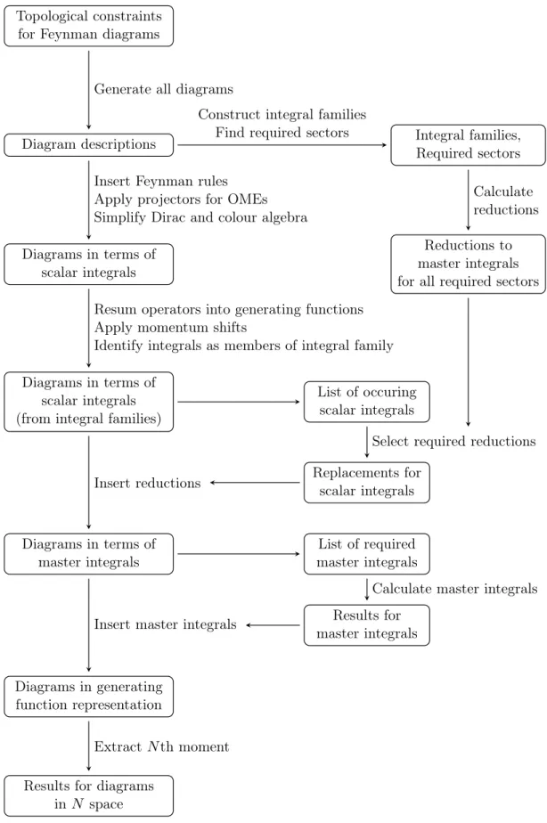
We calculate the OMEs in a diagrammatic approach, which involves generating Feynman diagrams and solving the associated Feynman integrals. To handle the large number of integrals, integration-by-parts identities [227–233] are used to eliminate relations among the integrals and to reduce them to a much smaller number of master integrals. These master integrals have to be solved and their results must be assembled into the result for the complete OME. We present an outline of the major steps involved in this calculation in Section 3.1 and collect some properties of the nested sums and iterated integrals which appear in the results in Section 3.2. Since one of the most demanding tasks is the calculation of the master integrals, we explain the techniques we use in Section 3.3. These methods include introducing a Feynman parametrisation and identifying the integrals as generalised hypergeometric functions and related functions [211–214, 234–239] to arrive at a sum representation or to use Mellin-Barnes integrals [208–210] to the same end. These sum representations are subsequently simplified in terms of nested sums using the summation algorithms [240–251], which are implemented in theMathematicapackagesSigma[241, 252, 253], EvaluateMultiSumsandSumProduction[254–257], as well asHarmonicSums[258–263]. Another important technique is the calculation of master integrals via differential equations [264–268]. We use a formal power series ansatz to translate the differential equations into difference equations and solve those by uncoupling them into a scalar recurrence and solving that in terms of nested

(14)

sums with the packages mentioned above.

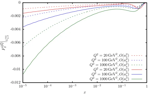
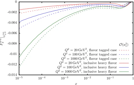
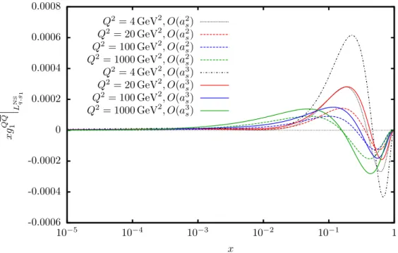
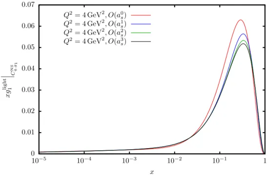
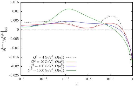
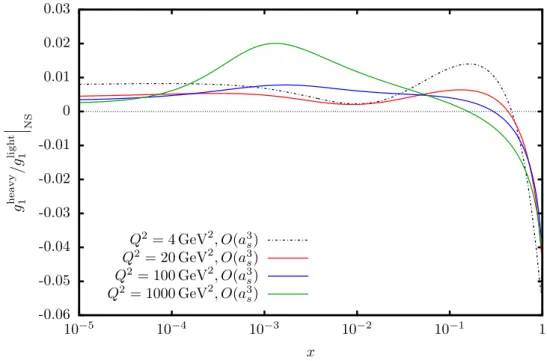
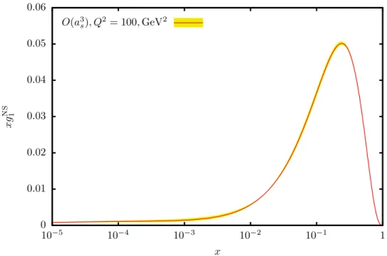
In Chapter 4, we apply the techniques to calculate the flavour non-singlet OME for even and odd values of the Mellin variableN. The even moments corresponds to the matrix element of the vector operator and the odd moments to the axial-vector operator. Moreover, we also calculate the OME of the tensor operator, which is relevant for the transversity structure functions. Besides the OMEs, we also obtain theN_F-dependent parts of the non-singlet anomalous dimensions. The OMEs enter the asymptotic factorisation of the heavy flavour Wilson coefficients for Q² m² and we discuss their influence on the unpolarised structure function F2(x, Q²), the polarised structure functiong₁(x, Q²)and the charged current structure functionxF₃(x, Q²). In the latter two cases, we also comment on the associated sum rules. Finally, we examine the non-singlet matching relation in the VFNS. Chapter 5 deals with the pure-singlet OME and its application.

We first present the calculation of the OME and of the pure-singlet anomalous dimension, which we obtain as a by-product of the calculation. This is the first independent recalculation of the pure-singlet anomalous dimension, which was first found in the massless case in [136]. We then give the pure-singlet asymptotic heavy flavour Wilson coefficient and illustrate its impact on the structure function F₂(x, Q²). Diagrams with ladder- and V-topology are an important class of diagrams which contribute to several OMEs. We select a sample of twelve diagrams from A⁽³⁾_Qg and discuss their calculation in Chapter 6. Here the method of differential equations plays a crucial role to calculate all required master integrals. Using similar methods, we also calculate theO ε⁰

term of the gluonic OMEA⁽³⁾_gg,Q in Chapter 7. This OME enters the matching relation for the gluon PDFs in the VFNS. In Chapter 8, we use the known fixed moments for the OMEs [193, 203] to compare the relative importance of the individual OMEs in the context of the heavy flavour Wilson coefficients and the VFNS. Chapter 9 contains the conclusions. The Feynman diagrams in this thesis have been drawn using Axodraw [269].

(15)

2. Deep-inelastic scattering

In this chapter, we review the basic formalism which is used to describe deep-inelastic scattering (DIS) processes in the context of quantum chromodynamics. In particular, we collect the definitions which lead up to the description of the contributions from heavy quarks in terms of operator matrix elements, since these are the quantities which we calculate here.

2.1. Kinematics of deep-inelastic scattering

The power of deep-inelastic lepton-hadron scattering lies in using stable, non-strongly interacting elementary particles to probe composite particles. The electro-weak interaction of leptons is well understood, which makes leptons excellent probes for the substructure of composite particles like hadrons. In a classical DIS experiment, a beam of leptons (electrons, muons or neutrinos) is shot at a fixed target or a second beam consisting of hadrons (usually protons or nuclear targets containing both protons and neutrons). The lepton then scatters off the hadron inelastically.

While the lepton is just deflected in this process, the hadron disintegrates into a complicated final state involving a number of particles. DIS is usually carried out as an inclusive experiment in which all possible hadronic final states that are allowed by quantum number conservation are taken into account. At lowest order of electro-weak theory, the lepton exchanges one electro-weak gauge boson with the hadron. This is the Born approximation and we will confine our discussion to this approximation, assuming that radiative corrections to the lepton system have already been carried out [270]. The gauge boson can be a photon, a Z⁰ or aW^± boson.

The kinematic situation is sketched in Fig. 2.1. An incoming lepton with four-momentum k= (E, ~k)scatters off a hadron with initial momentumP = (E_P, ~P)which results in a scattered lepton of momentum k⁰ = (E⁰, ~k⁰) and a hadronic final state carrying collective momentum P⁰. The scattering is mediated by exchange of one electro-weak gauge boson which carries momentum q =k−k⁰. Obviously, the momenta of the initial state hadron and of the initial and final state lepton are on their respective mass shells, k² =m²_` and k⁰² =m²_`0 andP² =M², wherem_`(`⁰₎ is the mass of the incoming (outgoing) lepton andM is that of the initial state hadron. Since the momentumP⁰describes a collection of particles, there is no on-shell condition for this momentum and we denote its invariant hadronic mass by W² =P⁰².

Several useful kinematic variables can be defined in a Lorentz-invariant way, which however take physically intuitive forms in certain reference frames. For two-particle scattering, the Man- delstam variable s, defined as

s= (P+k)², (2.1)

characterises the initial state and reduces to the square of the total energy in the centre-of- momentum frame. Since the gauge boson is exchanged in the t-channel, it has space-like momentum and its squared four-momentum q² is negative. Therefore, it is common practice to define

Q² =−q²=−(k−k⁰)² (2.2)

and to call this quantity the virtuality of the gauge boson. The name reflects the fact that in the case of photon exchange it measures how far off the mass shell (q² = 0) the boson is. In Born

(16)

Figure 2.1.: Sketch of the kinematic setup for deep-inelastic lepton-hadron scattering in Born approximation: The upper line denotes the lepton, the wavy line represents the electro-weak gauge boson and the lower line stands for the hadronic part of the reaction.

approximation it coincides with the Mandelstam variable tup to a sign, Q² =−t. We define ν as

ν = P.q

M = W²+Q²−M²

2M (2.3)

such that in the rest frame of the hadron (target system) it becomes the energy transfer from the leptons to the hadronic system,ν =E_TS−E_TS⁰ . Furthermore, it proves to be useful to define the Bjorken scaling variable [35, 271]

x= −q²

2P.q = Q²

2M ν = Q²

W²+Q²−M² (2.4)

and the inelasticity

y = P.q

P.k = 2M ν

s−M²−m²_` = W²+Q²−M²

s−M²−m²_` . (2.5)

In the target system, the inelasticity can be interpreted as the energy transfer from the lepton to the hadron system relative to the energy of the incoming lepton, y= (E_TS−E_TS⁰ )/E_TS.

The scattering process is called deep-inelastic if the virtuality Q² and the invariant mass of the final stateW² are sufficiently large. For nucleon (i.e. proton or neutron) targets a reasonable requirement is Q² ≥ 4 GeV² and W² ≥ 4 GeV² [272]. Below these limits there are significant contributions from nucleon resonances, while above them the continuum contribution dominates.

This continuum contribution is the matter of interest in DIS experiments, since it contains information about the internal structure of the hadron. For the discussions in this thesis, we neglect the masses of the leptons m_` = 0 and drop terms of order ^M²/Q². The latter are called target mass corrections and can become important at low values of Q² and large values of x [273–277]. Moreover, we will specialise the discussion to the case of nucleons in the initial state.

Both the leptons and the nucleons are spin¹/2 particles. The nucleon spin is described by the spin four-vector S, which we normalise as S²=−M². It fulfilsP.S= 0and can be decomposed into a longitudinal and transverse component with respect to the beam axis. In the nucleon rest frame the components take a particularly simple form if we align the z-axis with the beam axis, S_L=M(0,0,0,1), S_T =M(0,cos(β),sin(β),0), (2.6)

(17)

2.2. Cross section and structure functions

whereβ is the angle of the nucleon spin direction in the plane transverse to the beam axis.

For unpolarised scattering, there are three independent variables necessary to describe the kinematics of the scattering process. One variable describes the initial state for which we can choose for example the Mandelstam variable s. The two other variables, such as x and Q², characterise the final state configuration. If we describe scattering of polarised particles additional angular variables are necessary to describe the orientation of the spins.

The physical region of phase space is determined by a number of constraints. The total energy must account for at least the mass of the initial state nucleon, s≥M². Baryon number conservation requires at least one baryon in the final state which leads toW² ≥m²_p, wherem_p is the proton mass, since the proton is the lightest baryon. Moreover, for vanishing lepton masses, the virtuality must be non-negative, Q² ≥ 0, as must be the energy transfer to the hadronic system, ν ≥ 0. Then we deduce from Eq. (2.5) that 0 ≤ y ≤ 1. The limit y → 0 requires the energy transfer to the hadronic system ν to vanish, which corresponds to exact forward scattering. Considering proton scattering, we use

W²= (P+q)² =m²_p+Q²1−x

x ≥m²_p (2.7)

to show that 0≤x≤1. The elastic situation, whereW²=m²_p, corresponds to the limit x→1.

Since at most three kinematic variables can be independent, there are of course relations between the above invariants. A particularly useful one is

Q² =xy(s−M²)≈xys . (2.8) This allows to estimate the lowest attainable value ofx for a given virtuality. In particular, we get for HERA kinematics

x& Q²

10⁵GeV² . (2.9)

2.2. Cross section and structure functions

The calculations presented in this thesis concern the QCD corrections from massive quarks to inclusive deep-inelastic lepton-nucleon scattering. In particular, the results will be applied to three situations: Unpolarised scattering mediated by photons, photon-mediated polarised scattering and unpolarised scattering mediated by charged currents (W^± bosons). Therefore, we discuss the cross-sections which are relevant for these three cases and suppress contributions from weak neutral currents for brevity.

The matrix element for inclusive lepton-hadron scattering in the Born approximation of electro- weak theory reads [75, 76]

Mi = ¯u(k⁰, λ⁰)γ_µ(g_V,i+g_A,iγ₅)u(k, λ) e² Di(q²)

P⁰J_i^µ(0)P, S

, (2.10)

whereuandu¯are the Dirac spinors describing the initial and final state leptons with helicitiesλ and λ⁰, respectively. We denote the electromagnetic unit of charge byeand the Dirac matrices by γ_µ and γ₅, cf. also Appendix A. The nucleon initial state with momentum P and spin S has the state vector |P, Si and the hadronic final state is described by |P⁰i. Depending on the gauge boson that mediates the scattering, indicated by the index i, the vector coupling g_V,i, the axial-vector couplingg_A,i and the propagator factorD_i(q²)take different values. For photons we get

g_V,γ = 1, g_A,γ= 0, D_γ(q²) =q², (2.11)

(18)

while for W bosons they are

g_V,W^± = 1, g_A,W^±=−1, D_W^±(q²) = 2√

2 sinθW(q²−M_W² ), (2.12) whereM_W is the mass of theW boson and θW is the weak mixing angle. The current operator J_i^µ(0) is the electromagnetic (i = γ) or the weak charged current (i = W^±). The former is hermitianJγ^µ^†=Jγ^µ, while for the latter hermitian conjugation connectsW⁺ andW⁻ couplings by J_W^µ+ =J_W^µ^†−.

In order to obtain the differential cross section for inclusive scattering, we have to insert the squared matrix element into the cross section, sum over all allowed hadronic final states and integrate over their respective phase space. The form of the matrix element Eq. (2.10) allows us to decompose the cross section into a leptonic tensor L_µν and a hadronic tensorW_µν. First, we write this retaining all dependence on initial and final state spins [276, 278, 279]

d³σ(λ, λ⁰, S)

dxdydφ = yα² Q⁴

X

i∈{γ,W⁺,W⁻}

η_i(Q²)Lⁱ_µνW_i^µν. (2.13) Here α=e²/(4π)denotes the electromagnetic fine structure constant. If the polarisation of the final state lepton is not observed, we have to sum over its helicity states λ⁰. For unpolarised scattering, we also average over the spins of the initial state lepton and the nucleon, after which the integration over the azimuthal angle φof the scattered lepton becomes trivial. The normal- isation constants ηi(Q²) absorb the propagator factors and allow for a uniform notation across the different channels. They read

η_γ(Q²) = 1, (2.14)

η_W^±(Q²) = 1 2

G²_FQ⁴ (4π)²α²

M_W² Q²+M_W²

2

, (2.15)

whereGF is the Fermi constant which describes the weak strength of the interaction, G_F = e²

4√

2 sinθ_WM_W² . (2.16)

The leptonic tensor with all polarisation information is then given by Lⁱ_µν =

¯

u(k⁰, λ⁰)γ_µ(g_V,i+g_A,iγ₅)u(k, λ)_†

¯

u(k⁰, λ⁰)γ_ν(g_V,i+g_A,iγ₅)u(k, λ)

, (2.17)

which for unpolarised, photon-mediated scattering becomes 1

2 X

λ,λ⁰

L^em_µν = 2

k_µk_ν⁰ +k_νk⁰_µ−Q² 2 g_µν

. (2.18)

The same expression arises both for leptons and anti-leptons in the initial state. Keeping the polarisation information of the initial state lepton, but summing over the final state lepton polarisation λ⁰ yields the expression for polarised scattering

X

λ⁰

L^em_µν = 2

k_µk_ν⁰ +k_νk⁰_µ−Q²

2 g_µν+iε_µνρσ2λk^ρq^σ

. (2.19)

Finally, we give the expression for unpolarised charged current scattering, in which we average over λand sumλ⁰, but where there is an axial-vector coupling present,

1 2

X

λ,λ⁰

L^W_µν⁻ = 4

k_µk⁰_ν+k_νk_µ⁰ −Q²

2 g_µν+iε_µνρσk^ρk^0σ

. (2.20)

(19)

2.2. Cross section and structure functions

The hadronic tensor, on the other hand, contains the matrix element of the current operator between hadronic initial and final states. Since we have to sum or integrate over all unobserved degrees of freedom of the hadronic final state and since we sum over all allowed final states, we can use the completeness of states together with the positivity of the energy to write the hadronic tensor as a commutator of the currents between nucleon states,

W_µνⁱ (P, S, q) = 1 4π

Z

d⁴z e^iq.zhP, S|[J_µ^i†(z), J_νⁱ(0)]|P, Si . (2.21) A similar expression, where the current commutator is replaced by a time-ordered product, arises as the amplitude for Compton scattering of virtual photon with a nucleon for forward kinematics,

T_µνⁱ (P, S, q) =i Z

d⁴z e^iq.zhP, S|T[J_µⁱ^†(z)J_νⁱ(0)]|P, Si , (2.22) where T[. . .]is the time ordered product of its arguments. In fact, the two tensors are related by the optical theorem, see e.g. [75],

W_µνⁱ (P, S, q) = 1

2π ImT_µνⁱ (P, S, q). (2.23) At times, it is more convenient to deal with a time ordered product rather than the commutator of currents. By using translation invariance, one can also show that the crossing operationq→ −q, µ↔ν, which interchanges the initial and final state leptons, yields Tµν^γ (P, S,−q) =Tµν^γ (P, S, q) for the electromagnetic case, i.e. the amplitude is even under this operation. However, in the charged current case, the crossing operation acts on the Compton amplitude asT_νµ^W^±(P, S,−q) = T_µν^W^∓(P, S, q). In order to discuss objects with even or odd behaviour under crossing, it is useful to define the combinations, [280, 281],

T_µν^W⁺^±^W⁻ =T_µν^W⁺±T_νµ^W⁻, (2.24) which behave like T_µν^W⁺^±^W⁻(P, S,−q) =±T_µν^W⁺^±^W⁻(P, S,−q).

A direct evaluation of the hadronic tensor is not possible because of the strongly interacting, composite nucleon states. Nevertheless, we can parametrise it, using what is commonly known as structure functions, by making an ansatz using all possible Lorentz structures and imposing symmetry principles and conservation laws, see e.g. [272, 282]. In general, 14 independent structure functions are required to describe the hadronic tensor [276, 280] but under the assumptions made here, only five structure functions appear,

W_µν(P, S, q) = 1 2x

g_µν+qµqν

Q²

F_L(x, Q²) + 2x Q²

P_µP_ν+qµPν+qνPµ

2x − Q² 4x²g_µν

F₂(x, Q²) +iε_µνρσ

P^ρq^σ

2P.qF₃(x, Q²) +q^ρS^σ

P.q g₁(x, Q²) +q^ρ[(P.q)S^σ+ (S.q)p^σ]

(P.q)² g₂(x, Q²)

. (2.25) We choose to use the structure function F_L(x, Q²). An alternative choice would be to use F1(x, Q²) which is related toFL(x, Q²)and F2(x, Q²)by

F₁(x, Q²) = F₂(x, Q²)−F_L(x, Q²)

2x (2.26)

By contracting the hadronic and leptonic tensors and averaging over the initial state spins, we arrive at the differential cross section for unpolarised, photon-mediated scattering

d²σ^γ,unp dxdy =

Z _2π

0

dφ1 4

X

λ,λ⁰,S

d³σ^γ(λ, λ⁰, S) dxdydφ

= 2πα² xyQ²

1 + (1−y)²

F₂(x, Q²)−y²F_L(x, Q²)

. (2.27)

(20)

Thecrosssectionforpolarisedleptonsandhadrons,ontheotherhand,isgivenby d²σ^γ,po^l

dxdy =2πα²

Q⁴λ^p_Nf^psS^p₁(x,y)g1(x,Q²)+S₂^p(x,y)g2(x,Q²) , (2.28) whereλ^p_N denotesthedegreeofnucleonpolarisationandweusethefollowingshort-handsfor thecasesoflongitudinal(p=L)andtransversal(p=T)polarisationofthenucleon

f^L=1 f^T=cos(β−φ)dφ

2π 4M²x

sy 1−y−M²xy s S₁^L=2xy (2−y)−2M²

sxy S₁^T=2xy² S₂^L=−8x²yM²

s S₂^T=4xy. (2.29)

Theangleφistheazimuthalangleoftheoutgoingleptononwhichthereisanon-trivialde- pendenceinthecaseoftransversenucleonpolarisation.Inthiscase,βisthedirectionofthe nucleonspininthetransverseplane,seeEq.(2.6). Forunpolarisedchargedcurrentscattering, thediﬀerentialcrosssectionreads

d²σ^ν(¯^ν)

dxdy=G²_Fs 4π

M_W⁴ (Q²+M_W²)²

× 1+(1−y)² F₂^W^±(x,Q²)−y²F_L^W^±(x,Q²)± 1−(1−y)²xF₃^W^±(x,Q²) (2.30) d²σ^(¯)

dxdy=G²_Fs 4π

M_W⁴ (Q²+M_W²)²

× 1+(1−y)² F₂^W^∓(x,Q²)−y²F_L^W^∓(x,Q²)±(1−(1−y)²)xF₃^W^∓(x,Q²) . (2.31) The±signsrefertoincomingneutrinos(anti-neutrinos)orchargedleptons(anti-leptons). For calculationalpurposesitisadvantageoustoconsidercombinationsofstructurefunctionswhich haveanevenoroddbehaviourundercrossing. Toachievethis, wecanconsiderthesumor diﬀerenceoftheleptonandanti-leptoncrosssections,inanalogytoEq.(2.24). Weintroduce theshorthands

F₂^W⁺^+W⁻=F₂^W⁺+F₂^W⁻, F₂^W⁺^−W⁻ =F₂^W⁺−F₂^W⁻, (2.32) F_L^W⁺^+W⁻=F_L^W⁺+F_L^W⁻, F_L^W⁺^−W⁻ =F_L^W⁺−F_L^W⁻, (2.33) F₃^W⁺^+W⁻=F₃^W⁺−F₃^W⁻, F₃^W⁺^−W⁻ =F₃^W⁺+F₃^W⁻, (2.34) wherethecombinationsoftheleftcolumnappearinthesumofcrosssectionsandthecom- binationsoftherightcolumnappearinthediﬀerences. NotetheoppositesignsfortheF3

combinations.¹

1Weusetheconventionthatthesuperscript W⁺±W⁻referstothesumanddiﬀerenceofthecrosssections. Thisagreeswith[198],whiletheconventionof[153]referstothesumanddiﬀerenceofthestructurefunctions, whichexactlyswapsF₃^W⁺^+W andF₃^W⁺^−W .