https://doi.org/10.1007/s10236-019-01288-w
Processes affecting dissolved iron across the Subtropical North Atlantic: a model study
Anna Pagnone1 ·Christoph V ¨olker1·Ying Ye1
Received: 23 January 2019 / Accepted: 2 July 2019 / Published online: 26 July 2019
©The Author(s) 2019
Abstract
Trace metal measurements in recent years have revealed a complex distribution of dissolved iron (dFe) in the ocean that models still struggle to reproduce. The GEOTRACES section GA03 across the subtropical North Atlantic was chosen to study the driving processes involved in the Fe cycle in the region. Here, field observations found elevated dFe near the surface under the Saharan dust plume, a strong dFe minimum below the mixed layer depth, a maximum at the oxygen minimum zone near the African shelf, a hydrothermal maximum near the Mid Atlantic Ridge and lower dFe values in the deep eastern basin than in the west. We show that several of these features can be understood and be reproduced in models when they take into account scavenging on dust particles and phytoplankton, a variable ligand concentration and a hydrothermal dFe source. By doing so in a sequence of parameterisation changes, we are able to relate physical and biological processes, as well as internal and external dFe sources to observed features of the dFe distribution. In agreement with the observations, the additional scavenging on dust generates lower dFe concentrations in the deep eastern basin while the new ligand distribution results in a dFe maximum in the intermediate waters in the east basin and moderates the deep dFe gradient between the eastern and western basins.
Keywords Dissolved iron·North Atlantic·Biogeochemical model·Scavenging·Remineralisation·Ligands
1 Introduction
Iron (Fe) is an essential micronutrient for phytoplankton used to transfer electrons in key processes including photosynthesis, respiration, chlorophyll production and carbon and nitrogen fixation (Raven et al. 1999). Thus, Fe influences the marine biology from phytoplankton growth rate and community structure to higher trophic levels (Martin et al. 1994; Boyd et al. 2000; de Baar et al. 2005; Marchetti et al. 2006; Nicol et al. 2010).
Spatially, Fe regulates primary production in more than
Responsible Editor: J¨org-Olaf Wolff
Electronic supplementary material The online version of this article (https://doi.org/10.1007/s10236-019-01288-w) con- tains supplementary material, which is available to authorized users.
Anna Pagnone Anna.Pagnone@awi.de
1 Alfred Wegener Institute Helmholtz Centre for Polar and Marine Research, Am Handelshafen 12, 27570 Bremerhaven, Germany
25% (de Baar et al.2005) and up to possibly 50% (Moore et al. 2001; Boyd and Ellwood 2010) of the world’s oceans. The equatorial Pacific, the subpolar North Pacific and the Southern Ocean are the regions where biological productivity is mostly affected by the lack of Fe. Therefore, the global marine carbon drawn-down is significantly affected by Fe, making Fe one of the drivers of the oceanic carbon pump and inducing feedback effects on climate.
Most phytoplankton groups can only transport dissolved iron (dFe) over their cellular membrane, and many species have evolved intricate transporter systems for doing so (e.g. Lis et al. 2014). The cycling and distribution of dFe in the ocean is regulated by chemical, physical and biological processes. The main external inputs of dFe to the ocean are atmospheric dust deposition (e.g. Mahowald et al. 2005; Jickells et al. 2005), fluxes from reducing sediments (e.g. Elrod et al.2004) and hydrothermal vents (e.g. Resing et al.2015). Furthermore, Fe is introduced by river and groundwater erosion and discharge (e.g. Hunter et al. 1997) and by volcanic ashes (e.g. Hamme et al.
2010). In polar regions, glacial, iceberg (e.g. Raiswell et al.
2008) and sea ice (e.g. Lannuzel et al. 2008) meltwater are sources of Fe. Fe enters its biological cycle through
phytoplankton uptake, is transferred within the food web and is remineralised by heterotrophic organisms at depth.
Unlike other nutrients, dFe is additionally removed by scavenging on settling particles and vertical export of biogenic material from the water column (e.g. Balistrieri et al.1981), due to its extremely low solubility at seawater pH in the presence of oxygen (Liu and Millero 2002).
Ligands keep Fe in the dissolved phase (e.g. Gledhill and Buck 2012) to some extent mitigating its low inorganic solubility. Physical transport of dFe (and iron-binding ligands) by ocean currents, i.e. vertical mixing, upwelling of Fe-rich water masses or transport of specific ligand signatures, also influences the dFe distribution.
Large improvements have been made in the last decades in describing the global dFe distribution, and partly also that of organic Fe-binding ligands. The efforts of GEOTRACES, that have led to the 2017 IDP (Schlitzer et al.2018), have also revealed the importance of many new processes, such as the strong influence of hydrothermal vents on deep-sea dFe distributions.
However, many important processes affecting the Fe cycle are not well constrained quantitatively. Important examples are the strength of Fe sources to the ocean or the rate at which dFe is lost from the system through scavenging. Consequently, global biogeochemical models still differ much in their description of the marine Fe cycle, resulting in residence time estimates for dFe that vary over more than one order of magnitude (Tagliabue et al.
2016) and often in a much too homogeneous distribution of dFe in the deep ocean. The details of the distribution of dFe concentration that are obtained with GEOTRACES implicitly contain a wealth of information that can be used to constrain the quantitative representation of processes when combined with systematic parameter studies.
In this paper, we try to understand which processes deter- mine the dFe distribution in the Subtropical North Atlantic Ocean. The relevant local processes are scavenging on bio- genic and lithogenic particles, biological uptake, export and remineralisation. We have picked the GEOTRACES GA03 (Boyle et al.2015) cruise leg from Bermuda to Cape Verde as our study area. This region was chosen because it is a place of very intensive Fe cycling due to strong dust input and the flourishing biological activity in the Mauritanian upwelling region. Here, the processes of interest are more pronounced compared with other regions. In this process- oriented study on the GA03 cruise leg, we show how several details of the dFe distribution can be reproduced by intro- ducing new processes and by changing existing parameteri- sations of processes affecting the Fe cycle. The final model includes the effects of scavenging on dust and non-sinking biogenic particles, a non-constant ligand concentration and, for completeness, a hydrothermal dFe source. For better understanding, we present this output of a fairly extensive
parameter study by selecting only a simple sequence of steps in changing the model parameters that lead from our initial model setup to a final one. This presentation allows to discuss the contribution of the individual processes and parameterisation changes to the final outcome. As the Fe system reacts non-linearly to the parameterisation changes however, the magnitude of the changes in dFe distribution in the intermediate steps—but not in the final outcome—
is somewhat dependent on the sequence of changes. The succession of refinements intends to disclose the role of dif- ferent processes in controlling the distribution of dFe and their importance in biogeochemical models.
2 The GA03 section
The GEOTRACES GA03 cruise leg (Boyle et al. 2015) from Bermuda to Cape Verde took place in November 2011.
The aim of the cruise was to document the distribution of trace elements and isotopes in the region and to diagnose the nature of the controlling biogeochemical and physical processes. We focus on the dFe distribution (Sedwick et al.
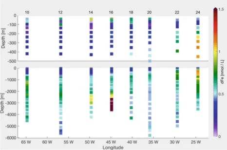
2015) (Fig.1) in the open ocean from station USGT11-10 to station USGT11-24 (Fig.S1in Online Resource).
The dFe concentrations (Fig.1) within the surface mixed layer are high, ranging between 0.37 and 0.98 nmol L−1 (or equivalentlyμmol m−3), caused by the North African dust flux (Hatta et al. 2015). The aerosol Fe from Saharan dust is predominantly released in the colloidal phase, having important implications for dFe availability to phytoplankton (Fitzsimmons et al.2015b). This appears to be representative of dFe in the tropical and subtropical surface Atlantic underlying the North African dust plume (Bergquist et al.2007; Fitzsimmons et al.2015a).
Across the gyre (Fig. 1), dFe displays a pronounced concentration minimum in the lower euphotic zone at the depth of the deep chlorophyll maximum (DCM). Such features have been previously reported in the subtropical and tropical North Atlantic (Sedwick et al.2005; Bergquist and Boyle 2006), and are supposedly caused by removal via biological uptake and particle scavenging (Fitzsimmons et al.2015b; Sedwick et al.2015).
In the intermediate waters at station USGT11-24 (Fig.1), no correlation between dFe and dissolved manganese was found, excluding sedimentary Fe from being the main source (Hatta et al.2015). This finding was also supported byδ56Fe measurements in Conway and John (2014). The correlation with the apparent oxygen utilisation (AOU) implies that the dFe maximum is here strongly associated with an addition of Fe via remineralisation alone (Hatta et al. 2015) (distributions of AOU and dissolved oxygen were reported in Jenkins et al. 2015). Model experiments by Pham and Ito (2018) argue that the intermediate water
Fig. 1 Measured dFe along GA03 (Sedwick et al.2015)
10 12 14 16 18 20 22 24
dFe [nmol / L]
dFe maxima are formed by the simultaneous release of scavenged Fe and ligands from organic particles.
Along the western edge of the transect (Fig.1), waters are enriched in dFe due to Fe advected from the North American continental shelf as part of the Upper Labrador Sea Water (Hatta et al. 2015) and are probably due to sedimentary resuspension. Below the thermocline, these elevated concentrations extend eastward beyond Bermuda.
In the intermediate and deep waters, the observations show a gradient between the east and the west basins, the latter having higher dFe concentrations (Fig.1).
A large dFe anomaly with a concentration of up to 68 nmol L−1 is observed at station USGT11-16 directly over a hydrothermal site. The hydrothermal signal extends at 2000–4000 m depth at least 500 km west of the Mid Atlantic Ridge (MAR) between 40◦W and 50◦W, with concentrations up to 1.13 nmol L−1, demonstrating that hydrothermalism contributes to the Fe pool in the deep ocean (Hatta et al.2015).
3 The model and its structure
In the model, the distribution of dFe is calculated from mass balance equations which take into account ocean circulation, the internal biogeochemical cycling of dFe and external dFe sources. The ocean circulation model that is used to calculate advective and diffusive tracer transport is the General Circulation Model of the Massachusetts Institute of Technology (MITgcm) (Marshall et al.1997).
Our setup covers the globe from 80◦S to 80◦N, excluding the Arctic, and has a zonal resolution of 2◦and a meridional resolution between 0.39◦ and 2◦. The thickness of 30 vertical layers increases with depth, from 10 m at the surface
to 500 m below 3700 m. The MITgcm is coupled with the marine ecosystem and biogeochemical model, REcoM2, described in detail in Hauck et al. (2013). REcoM2 describes two phytoplankton classes, diatoms and non- diatoms (small phytoplankton) with a variable elemental stoichiometry, following Geider et al. (2003) and Hohn (2009); a generic zooplankton class; and a class of organic particles sinking with vertically increasing velocity (Kriest and Oschlies 2008). The model experiments were set up with the same initial conditions and forcing fields as in Ye and V¨olker (2017).
3.1 Processes
Here, we describe the processes in our standard represen- tation of the Fe cycle. Some of them will change in the following sections.
The evolution of the dFe distribution over time is described by the following differential equation:
∂dF e
∂T = −(U+w)· ∇dF e+ ∇(k∇dF e)+S(dF e) (1) The first two terms on the right-hand side of Eq. 1 describe the physical transport and mixing by the system.
S(dFe)is the sum of all internal dFe sources and sinks (see Table1for symbol description):
S(dF e) =qF e((rphy−pphy)·Nphy+(rdia−pdia)·Ndia
+(rhet−εNhet)·Nhet
+ρNdet·fT ·Ndet)−kF escav·Cdet·F e (2) dFe is released by phytoplankton during respiration and by heterotrophs during respiration and excretion. Another internal source is remineralisation of sinking organic particles. dFe is drawn down by uptake of phytoplankton
Table 1 Table of parameters
Symbol Parameter Unit
U Advection velocity m day−1
w Sinking velocity m day−1
k Diffusivity m2day−1
F Dust flux mg m2day−1
rF e Iron in dust μmol Fe mg−1
sol Solubility −
dN Remineralisation rate of sediment organic N day−1
qBF e Benthic Fe:N ratio μmol Fe mmol N−1
qF e Fe:N ratio μmol Fe mmol N−1
rphy/dia/ het Phytoplankton/diatom/heterotroph respiration day−1
pphy/dia Phytoplankton/diatom N uptake rate day−1
Nphy/dia/ het /det /sed Phytoplankton/diatom/heterotroph/detritus/sediment N mmol N m−3
Cphy/dia/det Phytoplankton/diatom/detritus C mmol C m−3
εhetN Heterotroph excretion day−1
ρNdet Remineralisation rate day−1
fT Temperature-dependent Arrhenius function −
kscavF e Scavenging rate mmol C m−3day−1
kscavdustF e Lithogenic scavenging rate (mg m−3)−1day−1
F e Free iron μmol Fe m−3
Psmall/ large Small/large particles mg m−3
and by scavenging on sinking particles. External inputs are aeolian dust Fe and sedimentary Fe. The model considers neither riverine Fe input nor dFe from sea ice melting.
Parameters indicating the strength of individual processes are either taken from literature or are the result of sensitivity studies of the model.
Dust deposition The aeolian dFe source is a field of monthly averages of dust deposition (Mahowald et al.
2005). The flux to the ocean is:
k∂dF e
∂z
z=0=Fdust·rF e·sol (3)
The model assumes that 3.5% of dust particles consists of Fe and that 2% of this Fe immediately dissolves when deposited in the surface ocean.
Sediment source The sedimentary Fe source at the sea floor is given by the release of dFe proportional to the degradation of organic material in a homogeneous sediment layer:
k∂dF e
∂z
z=−H =qBF e·dN·P ONsed (4)
This goes back to Elrod et al. (2004), who found a significant correlation between the dFe flux from the sediment and the oxidation of organic matter. Sinking biogenic particles that reach the sediment are ultimately dissolved or remineralised and returned into the water
column as a normal flux, whereas the dFe scavenged is permanently removed.
Phytoplankton uptake In the model, the total pool of dFe is assumed to be bioavailable and the dFe uptake is proportional to nitrogen assimilation. The phytoplankton growth rate is limited by dFe, in the form of a Michaelis- Menten function, and by an intracellular nitrogen and silica quota.
Remineralisation In the first step of carbon or nitrogen remineralisation, the particulate organic matter (OM) is transformed into dissolved OM. Bacterial degradation then breaks it into dissolved inorganic carbon or nitrogen, which are bioavailable for phytoplankton. Since dFe is mostly organically bound anyway, the model returns Fe directly to the dissolved pool through remineralisation of particulate OM, with a rate ofρNdet· fT · Ndet.
Organic complexation The model considers two forms of Fe: the Fe bound to organic ligands, F eL, and the free inorganic Fe,F e. The Fe tracer in the model is the sum of the two formsdF e = F eL+F e.F e is calculated as in Parekh et al. (2004) and represents only a small percentage of the total dFe pool. It is assumed that Fe and ligands are bound in a 1:1 ratio. In REcoM2, the ligand concentration is assumed constant at 1μmol m−3 and the conditional stability constant is set to 1011.
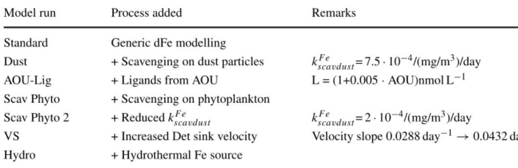
Table 2 Steps in model
development Model run Process added Remarks
Standard Generic dFe modelling
Dust + Scavenging on dust particles kF escavdust= 7.5·10−4/(mg/m3)/day AOU-Lig + Ligands from AOU L = (1+0.005·AOU)nmol L−1 Scav Phyto + Scavenging on phytoplankton
Scav Phyto 2 + ReducedkF escavdust kF escavdust= 2·10−4/(mg/m3)/day
VS + Increased Det sink velocity Velocity slope 0.0288 day−1→0.0432 day−1 Hydro + Hydrothermal Fe source
Scavenging The scavenging is assumed to be proportional to the detritus carbon, thus to the mass of sinking particles, and to theF econcentration,kF escav ·Cdet· F e.
3.2 Model experiments
Results of the FeMIP Project show many differences between Fe cycle models (Tagliabue et al.2016). However, some of the assumptions are similar, and the REcoM2 model shares many of them. Looking at the GA03 section, these result in an incomplete representation of the observations, where some important features of the dFe distribution are either not captured or their magnitude is misestimated. This may imply an inadequacy of the current Fe cycle modelling for the region in focus.
Different processes that affect the Fe cycle are often non-linearly dependent, meaning that a simple parameter- tuning exercise is difficult. For this reason, in the following, we show the changes in dFe concentration by introducing subsequently new processes in the model. Each model run was integrated for 1000 years from a state of rest. The five steps taken are from theStandardrun, to theDustrun which includes scavenging on lithogenic particles, to theAOU-Lig
run where a parameterisation of ligands was introduced, to the Scav Phyto run in which an additional scavenging on phytoplankton was added, to theVSrun where the velocity of sinking particles is changed, to the finalHydrorun which includes a hydrothermal dFe source (Table2). The details of these changes are explained in Results (Section4).
4 Results
4.1 StandardIn the Standard run the scavenging rate is kscavF e = 0.02 mmol C m−3d−1. The model shows (Fig.2) high dFe concentrations at the surface of the east basin (east of the MAR—east of 45◦W) due to strong aeolian input from the African continent. This influences the layers below until ca. 300 m depth. In the west basin (west of the MAR—west of 45◦W), we see a minimum at ca. 50 m, which corresponds to the DCM and is an expression of biological dFe uptake.
Both these features are also seen in the GEOTRACES data (Fig. 1). However, compared with the observations, the model generally overestimates dFe. Near the American
Fig. 2 Modelled dFe along GA03 in theStandardrun, with measured dFe values as dots
dFe [nmol / L]
coast at 200–300 m, a dFe maximum is observed in the model which is not seen in the data (Fig.2). This dFe is transported north from the region off Puerto Rico. Below 500 m, the dFe concentration is fairly homogenous in the model, slightly lower on the west side of the MAR.
The model does not reproduce the dFe variability in the intermediate and deep ocean: one reason being that the hydrothermal dFe input is neglected here.
4.2 Standard + dust scavenging
In the Subtropical North Atlantic, scavenging on lithogenic particles is a major process in the Fe cycle. Ye and V¨olker (2017) argue that neglecting dust particles as scavengers is one main reason for overestimation of dFe under the Saharan dust plume. The particle dynamics in
the model considers aggregation and disaggregation of fine dust particles and large organic and lithogenic particles.
Scavenging now occurs on lithogenic particles as well as organic particles (2):
(kF escav·Cdet+kscavdustF e ·(Psmall+Plarge))·F e (5) where kscavdustF e = 7.5·10−4(mg m−3)−1d−1 (Table 1). For further details, see Ye and V¨olker (2017).
Including removal by lithogenic particles reduces the dFe concentration everywhere in the transect (Fig.3). The largest effect occurs in the water column under the dust plume where the water in the upper 100 m loses 30% of dFe, whereas the intermediate and deep waters lose 70% of dFe.
While in the Standard run the scavenging loss of surface dFe is limited to the upper 50 m and east of
Fig. 3 aModelled dFe concentration in theDustrun along GA03, with measured dFe values as dots;bdFe difference between theStandardrun and theDustrun
dFe [nmol / L]dFe [nmol / L]
a
b
26◦W, reaching a maximum of 4.5 nmol L−1year−1, the effect now is more widespread, reaching as far as 40◦W, and into the oligotrophic waters of the subtropical gyre at a 100-m depth. The scavenging strength reaches here a maximum of 12 nmol L−1year−1. Consequently, the dFe concentration is reduced by more than 1 nmol L−1 between 25◦W and 40◦W (Fig. 3b), but it is still too high compared with the observations. Here, the biogenic and lithogenic scavenging is the most dominant process affecting dFe distribution compared with biological uptake and remineralisation as can be seen in the upper layers in the east basin (ED1) in Fig.S2in Online Resource where the integrated contributions of scavenging, biological uptake and remineralisation to the dFe pool are shown.
Alterations in the surface dFe distribution caused by the additional scavenging onto dust particles were already observed by Ye and V¨olker (2017). However, the changes are not limited to the surface ocean: while the Standard run gives homogenous dFe concentrations below 500 m, the scavenging on dust introduces longitudinal structure, showing a strong gradient between the east and the west basins (Fig.3). A similar but weaker gradient was also seen in the observations (Fig. 1). dFe in the model decreases in the east basin by roughly 0.6 nmol L−1, and by only 0.15 nmol L−1 in the west basin, with the result that the dFe concentrations in the east basin are too low. It should be noted that here we used the same dust scavenging rate and aggregation and disaggregation coefficients as in Ye and V¨olker (2017). With more data for particles in different size fractions, a full sensitivity study on the aggregation and disaggregation rate could be performed.
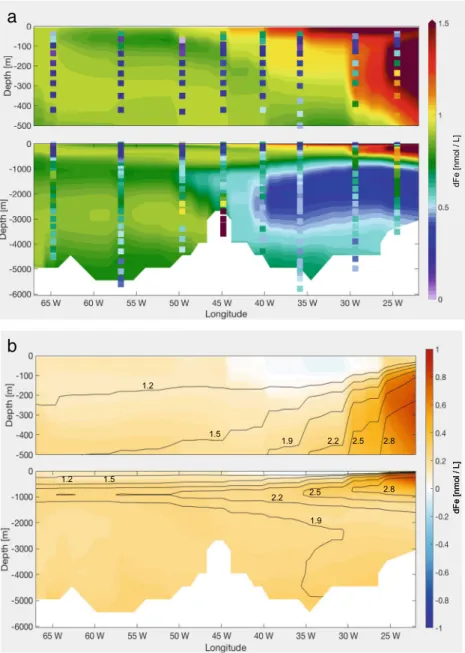
4.3 Standard + dust scavenging + AOU ligands The eastern part of the GA03 shows a dFe maximum between 300 and 600 m where an oxygen minimum zone (OMZ) spreads from the Mauritanian coast (Fig.1). This pronounced OMZ has shown a correlation to the elevated dFe concentrations in this particular region (Rijkenberg et al. 2012). Here, remineralisation of sinking organic material releases both dFe and organic ligands which prevent dFe from scavenging removal. Previous studies also ascribed the dFe maximum along GA03 to remineralisation processes (Hatta et al.2015), dissociation of adsorbed Fe from sinking particles and ligands from organic particles (Pham and Ito2018).
Our model runs, however, do not reproduce this feature, despite having a strong remineralisation of dFe. Based on the strong correlation between AOU and dFe in GA03 (Hatta et al. 2015), we decided to introduce a ligand parameterisation based on AOU in a similar way to Misumi et al. (2013), who applied a linear relationship between AOU and the weak binding ligands L2. Comparing the
AOU values from the World Ocean Atlas (Garcia et al.
2010a) with the ligand data along GA03 (Buck et al.
2015), we notice a correlation between AOU and the strong binding ligands L1, rather than L2. The Pearson correlation coefficient is 0.45 when using ligand data between 200 and 3000 m depth. This emphasises that oxidation of OM is an important source of ligands. Instead of using a constant ligand concentration of 1 nmol L−1, we adapted the parameterisation of Misumi et al. (2013) to represent the abundance of total ligands in theAOU-Ligrun:
L=1nmol L−1+0.005nmol L−1
μmol L−1 ·AOU (6) where 0.005 is the slope of the fit between AOU and L1.
The new ligand distribution changes in a similar way to dFe in Fig. 4. It is reduced to ca. 0.95 nmol L−1 at the surface; east of 30◦W between 200 and 1000 m the concentration is now higher than 2 nmol L−1; a tongue of ca. 1.5 nmol L−1 ligand’s concentration extends at 1000 m from the east to the west; the average concentration below 2000 m in the east basin is 1.5 nmol L−1, while in the west basin it is 1.3 nmol L−1. Since the ligand concentration becomes higher than 1 nmol L−1 everywhere but at the surface, we see a lower scavenging loss and an average increase of dFe concentrations of 0.3 nmol L−1 along the transect (Fig. 4). East of 26◦W, at the depth of the AOU maximum, the dFe concentrations are on average 0.8 nmol L−1higher than theDustrun, stretching vertically from the surface to 500 m. Below 1000 m, the increase of dFe is 150% in the east basin, which had before a too low iron concentration, and only of 50% in the west basin.
A limitation of this ligand parameterisation is that it can not be applied globally. This parameterisation is an approximation for younger water masses like the deep Atlantic Ocean, but leads to too high ligand concentrations in older water masses such as in the deep Pacific Ocean (not shown) (Section 5.4).
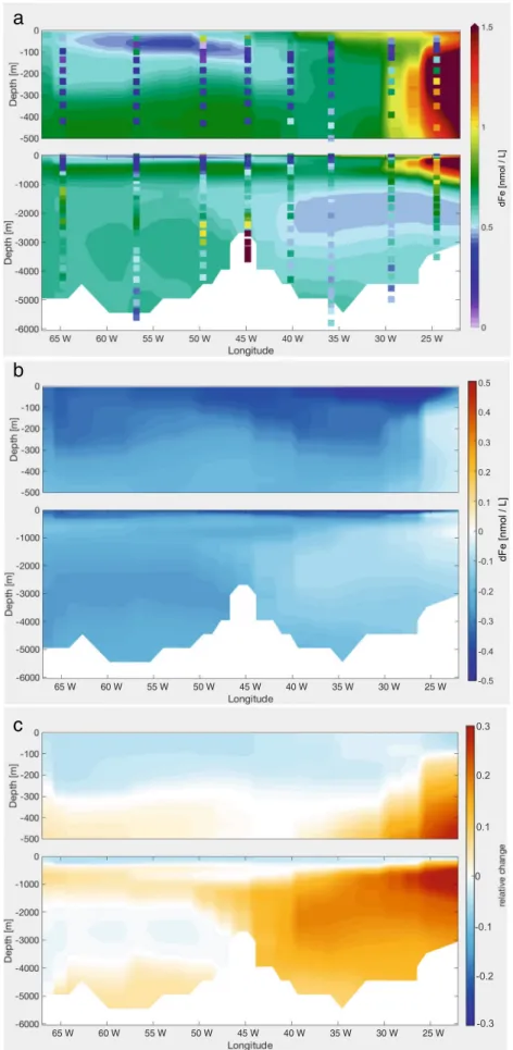
4.4 Standard + dust scavenging + AOU ligands + phytoplankton scavenging
A strong subsurface dFe minimum occurs within the centre of the North Atlantic subtropical gyre and stretches across the Atlantic basin. The minimum at the DCM between 100 and 200 m is argued in the literature to be caused by combined dFe scavenging and biological uptake (Hatta et al.2015). As described in Section4.1, theStandardrun does reproduce a subsurface minimum; it is however not pronounced enough. Since the modelled primary production in this region is comparable with observations, we take a closer look at the scavenging process. Phytoplankton can be considered as small particles which offer a surface to
Fig. 4 aModelled dFe along GA03 in theAOU-Ligrun, with measured dFe values as dots;b dFe difference between theDust run and theAOU-Ligrun. The contour lines show the new ligand concentration (nmol L−1)
a
b
dFe [nmol / L]dFe [nmol / L]
1.2
1.5 1.9 2.2 2.5 2.8
1.2 1.5
1.9
2.2 2.5 2.8
dFe [nmol / L]
scavenge dFe (Hudson and Morel 1989). In Eq. 2, the scavenging term is (Table1):
(kscavF e ·(Cdet+Cphy+Cdia)+kF escavdust·(Psmall+Plarge))·F e (7) The dFe concentration is reduced everywhere along GA03 (Fig. 5), with the major effect in the upper 100 m, with the maximal dFe loss of 0.5 nmol L−1. Here, introducing scavenging on phytoplankton leads to a scavenging increase between 50 and 300% between 45◦W and 65◦W. Though scavenging on phytoplankton is limited to the euphotic zone, we also observe a decrease of dFe in the deeper layers. This is caused by a decrease in the pre-formed dFe concentration in the water mass formation regions.
To prevent an overly low dFe at depth, we reduce the scavenging rate of dust particles, kF escavdust, to 2·10−4(mg m−3)−1day−1 (Scav Phyto 2 run) (Fig. 5c).
This mainly affects the deep east basin, where the average concentration of 0.3 nmol L−1 is increased to ca. 0.5 nmol L−1, since more dFe sinks to the deep ocean by reducing the scavenging under the dust plume. The west basin is almost unchanged due to the limited influence of dust in this region.
The observed dFe shows very low concentrations also below the DCM, where the dFe concentration is expected to increase again due to remineralisation. The low dFe concentrations extend down to 700 m (Fig.1). Neither the Standard run nor the Scav Phyto 2 run reproduces this feature; the reason is discussed in Section5.3.
Fig. 5 aModelled dFe the GA03 in theScav Phytorun, with measured dFe values as dots;bdFe difference between theAOU-Ligrun and theScav Phytorun;cdFe difference between theScav Phytorun and theScav Phyto 2run
dFe [nmol / L]
65 W 60 W 55 W 50 W 45 W 40 W 35 W 30 W 25 W
dFe [nmol / L]
0.5 0.4 0.3 0.2 0.1 0 -0.1 -0.2 -0.3 -0.4 -0.5
65 W 60 W 55 W 50 W 45 W 40 W 35 W 30 W 25 W
0.3
0.2
0.1
0
-0.1
-0.2
-0.3
a
b
c
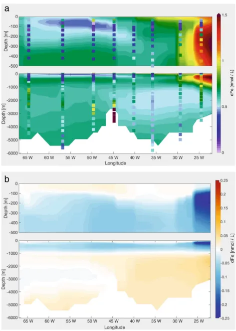
4.5 Standard + dust Scavenging + AOU ligands + phytoplankton scavenging + increased velocity slope
The observed intermediate water dFe maximum, which is mainly driven by remineralisation, is deeper compared with the modelled one. In addition, the vertical maximum of dissolved inorganic nitrogen (DIN) in the model is shallower than the observations in WOA (Garcia et al.
2010b), indicating that also the remineralisation process in the model is too shallow. The depth of remineralisation depends on how fast organic particles sink. In the model, the sinking speed of detritus is 20 m day−1 at the surface and increases linearly with depth after Kriest and Oschlies (2008) with a slope of 0.0288 day−1. To deepen the remineralisation flux, we increased the slope of the sinking
velocity by 50%, to 0.0432 day−1, so that biogenic particles sink out of the surface, and the water column, faster.
In the upper 100 m, this results in a slight increase of 5%
in dFe concentration along the transect (Fig.6), despite an increase of scavenging and a decrease in remineralisation.
The biological production in the Subtropical North Atlantic Ocean is macro-nutrient limited. Increasing the sinking velocity of particles, the residence time of organic particles in the water column is reduced and so the remineralisation of nutrients, leading to an intensified nutrient limitation of phytoplankton growth. This induces a weaker biological production, thus weaker uptake of dFe, leaving more dFe in the water. At the same time, increasing the sinking velocity means that large particles remain a shorter time in the upper water column, while small particles increase due to less aggregation. The dFe removal by scavenging is
Fig. 6 aModelled dFe along GA03 in theVSrun, with measured dFe values as dots;b dFe difference between theScav Phyto 2run and theVSrun
dFe [nmol / L]
65 W 60 W 55 W 50 W 45 W 40 W 35 W 30 W 25 W
dFe [nmol / L]
a
b
reinforced by this higher concentration of small particles.
The competition of these two processes leads to different features west and east of 26◦W. West of 26◦W, the dFe loss term at the surface is dominated by biological uptake compared with scavenging, explaining the dFe increase in the upper 100 m. On the other hand, east of 26◦W, under the dust plume, scavenging is mainly controlling dFe concentration. Here, the dFe concentration is reduced.
Between 100 and 1000 m, dFe decreases while below it increases, both ranging from 5 to 15%, with a maximal effect in the east. The mean scavenging is reduced by approximately 5% below 200 m, except east of 26◦W where it is reduced by 40%. In general, the mean remineralisation in this run is reduced by 20 to 40% in the upper 1000 m (Fig.S3and Fig.S2, e.g. ED1 and ED2), while it increases by the same amount below 1000 m. West of 65◦W, the remineralisation increase reaches 80% (Fig.S3and partially seen in Fig.S2, WD3). This does not only affect local dFe profiles but also the entire Fe cycle because of the longer residence time of dFe.
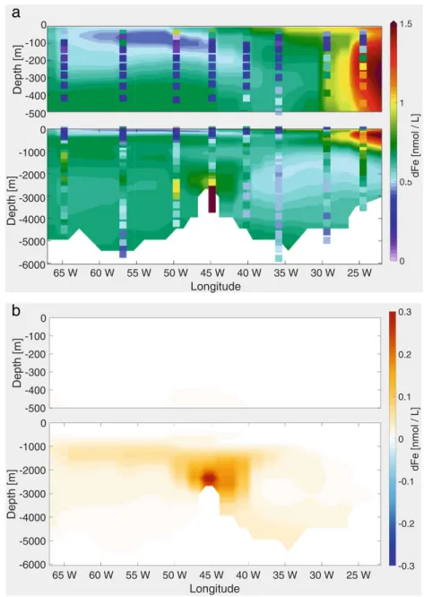
4.6 Standard + dust scavenging + AOU ligands + phytoplankton scavenging + increased velocity slope + hydrothermal vent
The measurements of GA03 show a strong hydrothermal dFe input from the MAR at 45◦W (Fig. 1). Though the representation of hydrothermal vents as a source of dFe to the deep ocean is not new (Tagliabue et al. 2010), we present the result of theHydrorun here as an additional and final step since the effect of each process investigated in this study on the dFe distribution does not add on linearly.
As Tagliabue et al. (2010), we assumed proportionality of the release of dFe to that of 3He at known position of hydrothermal vents. The distribution of hydrothermal vents used in the model includes a vent site located about 1◦to the west of station USGT11-16. The uncertainty of the location of hydrothermal vents and in the proportionality of dFe to
3He has to be mentioned.
TheHydrorun was started from the output of theVSrun after 900 years and was then integrated for a further 100 years to include the local hydrothermal effect. The effect of the hydrothermal source of dFe is strongly influenced by the AOU-based ligand parameterisation, thus switching on the hydrothermal source in combination to the new ligand distribution for longer integrations leads to a non- local signal in our setup—in Section5.4, this topic will be discussed.
As expected, in the model, a far field plume of high concentrations up to 0.9 nmol L−1is expanding at a depth of 2000 to 3000 m, up to 5◦ east and 5◦ west of the source (Fig. 7). The lateral spreading of dFe over large distances, which has been observed in the GEOTRACES
program, has been ascribed to the concomitant release of organic ligands (e.g. Bennett et al.2008) or the formation of microparticles which hardly sink (e.g. Y¨ucel et al.
2011) and which possibly exchange Fe reversibly with the dissolved phase (Fitzsimmons et al.2017). Neither of these processes is present in the model. The extremely high values observed at station USGT11-16 in the buoyant plume, up to 68 nmol L−1, can not be represented by models with coarse resolution, where dFe is homogeneously mixed in the bottom box. Such high point values are important for the first scavenging loss in the near field of vents but not for biogeochemistry at the scale of model resolution.
5 Discussion
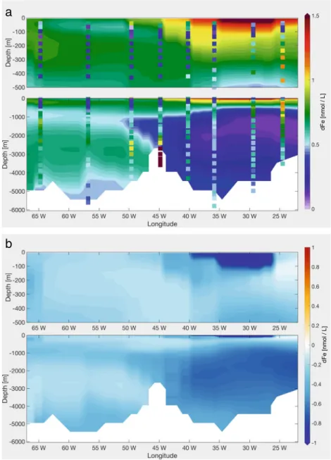
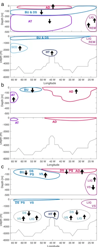
The dFe concentrations along GA03 give indications on which processes are important in shaping its distribution in the Subtropical North Atlantic. The main features and their controlling processes can be summarised (Fig. 8a): (1) A strong aeolian deposition leads to surface dFe maximum;
(2) in the lower euphotic zone, the dFe concentration is very low due to biological uptake and scavenging onto biogenic and lithogenic particles; (3) between 200 and 1000 m east of 30◦W, the elevated dFe concentration is determined by remineralisation and high ligand concentration; (4) at the west edge, between 200 and 700 m, dFe-poor water is advected from the north; (5) close to Bermuda, a dFe increase between 1000 and 2000 m is observed in correspondence of sedimentary dFe-rich water transported from the Upper Labrador Sea; (6) extremely high dFe concentrations are found over and around the hydrothermal vents on the Mid Atlantic Ridge.
These features and processes are not well represented in ourStandard run (Fig. 8b): (1) The dFe concentrations at the surface are overestimated; (2) only a much weaker dFe subsurface minimum is found; (3) no dFe maximum is reproduced close to Cap Verde between 200 and 1000 m;
(4) close to Bermuda, between 100 and 300 m, the model features dFe-rich water advected from the south; (5) the model does not reproduce the dFe variability in the intermediate and deep ocean, as below 500 m the dFe concentration is almost constant.
The steps undertaken in this study to improve the understanding of key processes as well as the model-data agreement are as follows: including scavenging by both lithogenic particles and phytoplankton (Sections 4.2,4.4);
keeping remineralised dFe in solution by moving from a constant ligand distribution to one which has higher ligand concentration in the OMZ (Section4.3); deepening the Fe remineralisation by accelerated sinking of biogenic particles (Section 4.5); considering the hydrothermal dFe source (Section4.6).
Fig. 7 aModelled dFe along GA03 in theHydrorun (100 years), with measured dFe values as dots;bdFe difference between theVSrun and the Hydrorun (100 years)
-500 -400 -300 -200 -100 0
Depth [m]
65 W 60 W 55 W 50 W 45 W 40 W 35 W 30 W 25 W Longitude
-6000 -5000 -4000 -3000 -2000 -1000 0
Depth [m]
-0.3 -0.2 -0.1 0 0.1 0.2
dFe [nmol / L]
65 W 60 W 55 W 50 W 45 W 40 W 35 W 30 W 25 W Longitude
-500 -400 -300 -200 -100 0
Depth [m]
-6000 -5000 -4000 -3000 -2000 -1000 0
Depth [m] dFe [nmol / L]
0.3
a
b
The final model setup describes the dFe distribution in the Subtropical North Atlantic more realistically (Fig.8c).
The dFe surface concentration is mainly regulated by dust and phytoplankton scavenging, with the major effect under the dust plume. The effect of phytoplankton scavenging is widespread and generates a subsurface dFe minimum.
Relating ligand concentration to AOU increases the dFe concentration mostly east of 26◦W. Even though the dFe values shown here are too high compared with the observations (Fig.4), with this parameterisation of ligands, we are able to reproduce the local vertical maximum.
Increasing the sinking velocity of the biogenic particles, the remineralisation source of dFe is shifted towards depth with a decrease of dFe concentration between 100 and 1000 m and an increase below. At depth, the scavenging on dust introduces longitudinal structure which is somewhat
mitigated by a gradient in ligand concentrations. The local hydrothermal input leads to high concentrations above the vent, even though not as high as in the measurements.
While Fig.8a, b and c show the qualitative effects of each new process on the dFe distribution, a more quantitative approach is given in Section 1 and Fig. S2 in Online Resource.
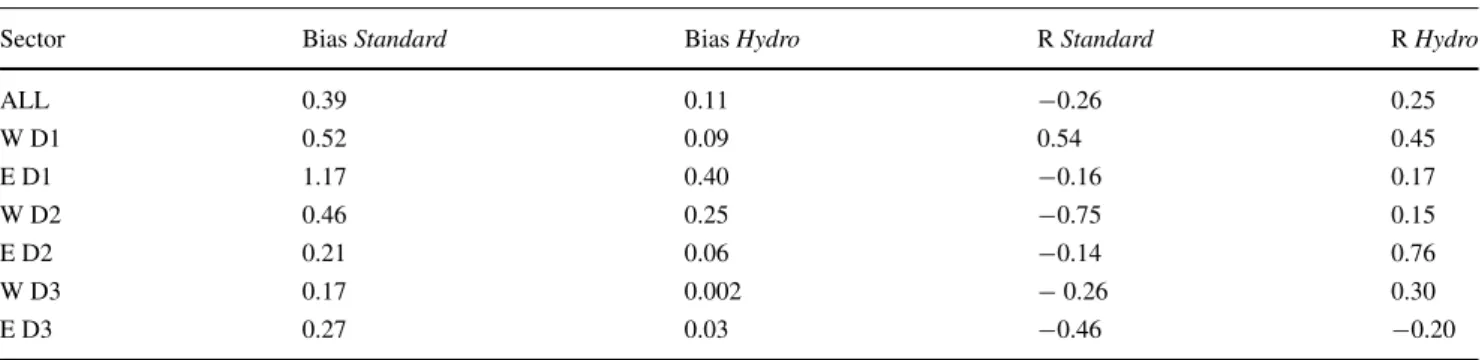
5.1 Statistical assessment
We examined the Pearson correlation between the observed and modelled dFe at the same locations in the initial Standardrun and the finalHydrorun (Table3). Taking into account the entire water column along GA03, the correlation coefficient between modelled and observed dFe is R =
−0.26 in theStandard run and it improved toR = 0.25
Fig. 8 Pattern of dFe in the observations a, in the Standard run b and in the Hydro run c. The most important processes which influence the dFe distribution are as follows: AD, aeolian deposition;
HT hydrothermal input; BU biological Uptake; DS dust scavenging;
LIG ligand binding; REM remineralisation; SED sedimentary input;
AT advective transport; PS phytoplankton scavenging; VS sinking velocity. The arrows indicate whether the process is a source or a sink of dFe
in the Hydro run. The mean bias against observations is reduced from 0.39 to 0.11 nmol L−1.
To better analyse the local effects of the processes, we split the section into six sectors by considering east and west basins (east and west of 45◦W), and by defining three depth layers, being D1 from the surface to 200 m, D2 from 200 to 1000 m and D3 from 1000 m to the sea floor. In each sector, the biases are notably reduced by 46 to 99%, indicating that the model output of theHydrorun is much closer to the observations than the initialStandard run. The smallest biases are found in both basins below 1000 m, indicating that the model now produces a realistic deep east–west gradient. Almost all correlation coefficients increase, in some cases however just moving from an anticorrelation to no correlation. The D2 depth stratum in the east basin shows the highest correlation (R = 0.76) due to the new ligand parameterisation, followed by D1 in the east basin with R = 0.45. The improvement in the deep layer was obtained by examining the effect of scavenging on dust at depth, which first introduced an inter- basin gradient. Additionally, considering the hydrothermal dFe input enabled a better agreement around 45◦W. Here, the relative standard deviation (σ (obs)/σ (mod)) in the east and west basins is reduced in the Hydro run by 82 and 68%, respectively, pointing out that the solution for the too homogenous dFe distribution in the model has come closer.
5.2 Surface dFe
Saharan dust outbreaks occur episodically and their trajec- tories change with the seasonal and latitudinal fluctuations of the Intertropical Convergence Zone (Chiapello et al.
1995), affecting surface dFe concentration. Available mea- surements (Tagliabue et al. 2012; Schlitzer et al. 2018) between 10◦N and 40◦N (Fig.S4in Online Resource) show strong variability, both with longitudinal location and the month of sampling (Fig.9). The data were compared with dFe output from the Standard run, the Dust run and the Scav Phyto 2run, those runs which have shown to mostly affect the surface concentration. In each run, we considered the monthly dFe minimum and maximum within the lati- tude band from 10 to 40◦N. The observations should lay in the range of latitudinal–temporal variability defined by the minimum and maximum modelled dFe.
TheStandardrun maximum (Fig.9) has low dFe values at the American coast, an increase in the open ocean, a decrease around ca. 23◦W and very high dFe value between 20◦W and the African continent.
The effect of dust scavenging (Dust run) depends on the relative amount of biogenic and lithogenic particles.
Close to the American coast, the biological productivity is comparatively high and dust deposition is small; thus, the Dust run reduces dFe by only 15% (Fig. 9). The dFe
Table 3 Model statistics: bias (nmol L−1) and correlation coefficient (R) between the observed and modelled dFe in theStandardrun and the Hydrorun
Sector BiasStandard BiasHydro RStandard RHydro
ALL 0.39 0.11 −0.26 0.25
W D1 0.52 0.09 0.54 0.45
E D1 1.17 0.40 −0.16 0.17
W D2 0.46 0.25 −0.75 0.15
E D2 0.21 0.06 −0.14 0.76
W D3 0.17 0.002 −0.26 0.30
E D3 0.27 0.03 −0.46 −0.20
W, west of 45◦W;E, east of 45◦W;D1, 0–200 m;D2, 200–1000 m;D3, 1000–6000 m
concentration in the subtropical gyre between 25◦W and 65◦W, where biology is weak, is reduced by 45% and the maximum east of 20◦W, where productivity and dust deposition are both high, is reduced by 25% .
Adding variable ligands and scavenging on phytoplank- ton (Scav Phyto 2run) (Fig.9), further scales down the max- imum dFe concentration in the region by 14% in the west, 32% in the centre and 13% in the east, where scavenging is 10% less than that in the centre.
The monthly minima do not differ much in the three model runs.
Both changes bring the model much closer to the measured surface values, even though the model still overestimates the dFe concentration directly under the Saharan dust plume. A reason could be that our model does not include a direct removal of dFe via ‘colloidal pumping’
(Honeyman and Santschi 1989), i.e. the fast aggregation of colloidal particles with larger particles. Aerosol Fe is predominantly released into the colloidal size fraction (Section2) (Fitzsimmons et al.2015b). Therefore, we could
be missing an important loss process of dFe. Furthermore, in our model, the input from dust deposition is calculated with an uniform solubility of 2%, while it has been shown that Saharan’s dust solubility is smaller because of its mineralogy and small anthropogenic contribution (Bonnet and Guieu 2004). Considering a variable solubility in the model might further improve the model-data agreement.
5.3 Subsurface dFe
The GA03 exhibits very low subsurface dFe concentrations at depths between 100 and 200 m and extending to 700 m in the western basin, implying a remarkably strong dFe sink which draws down almost all dFe deposited at the surface. The decrease of dFe to low concentrations between 30 and 70 m is associated with the DCM and is explained by removal mechanism as a strong biological uptake and scavenging on phytoplankton (and maybe colloidal aggregation which however is not included in our model).
Below the DCM, we would expect an increase in dFe;
Fig. 9 Latitudinal-temporal variability of observed and modelled surface dFe. For each model run (Standard,Dustand Scav Phyto 2), 12 lines represent the monthly maximum and further 12 lines represent the monthly minimum
however, west of 35◦W, the dFe concentrations remain low until ca. 700 m. Bergquist and Boyle (2006) point out this broad dFe minimum to be characteristic for dFe profiles in the North Atlantic subtropical gyre and to be enclosed in a pycnocline as deep as 700 m. Jenkins et al.
(2015) show that the thermocline waters in the GA03 section lie between the winter mixed layer and the density boundaryσ0= 27 kg m−3, which separates them from the intermediate water masses. Theσ0 density boundary lies roughly between 600 and 800 m. Along the section, 90% of the thermocline waters’ end member water types consists of the North Atlantic Central Waters. At the outcrop of this water (ca. 40◦N) (Tchernia1980), dust deposition is lower, and therefore water masses have potentially lower surface dFe values. This water then spreads along isopycnals towards the subtropics.
In theHydrorun (Fig.7), the subsurface dFe minimum is present but only extends to a depth of ca. 200 m. Below, dFe increases, instead of maintaining very low observed values.
In the model, the isopycnalσ0= 27 kg m−3 along GA03 is found at similar depths as in Jenkins et al. (2015), thus the modelled water mass is formed approximately at the same latitude as the observed. Despite the dust deposition in the North Atlantic is relatively low in the model, the modelled dFe concentrations north of GA03 section along the isopycnal (Fig.10) are too high compared to the observed values along GA02 (Rijkenberg et al. 2014). Most likely, this is due to a surface northward advective transport from the subtropical gyre characterised by too high dFe under the dust plume. Other explanation could be a still too shallow remineralisation, a too low consumption by phytoplankton
and higher Fe:C. The first was tested in the VS run and the latter is discussed in Section 2 in Online Resource.
Fitzsimmons et al. (2013) derived Fe:C rations ranging between 9.6 and 12.4μmol/mol, which agrees with previous findings by Bergquist and Boyle (2006) (11μmol/mol). The enriched Fe:C ratio in the tropical North Atlantic could reflect “luxury uptake” by phytoplankton, thus the storage of dFe for future dFe-poor times (Fitzsimmons et al.2013).
By any means, the southward transport of these water masses along the isopycnal leads to an overestimation of the subsurface dFe concentration in our model.
5.4 Intermediate and deep dFe
In the intermediate and deep waters, the dFe concentration is determined by remineralisation, ligand concentration, transported water enriched with sedimentary dFe and hydrothermal dFe input. Additionally, we observed that scavenging on lithogenic particles, which has mostly been analysed in relation to surface dFe distribution (Ye and V¨olker2017), also has a great effect at depth. Indeed, in the Dust run, the very homogenous dFe concentrations below 1000 m in theStandard run are replaced by an inter-basin gradient. Scavenging at depth is smaller than at the surface right under the dust plume; however, the relative change is maximal in the deep waters in the east basin. Here, the dFe decreases by three orders of magnitude because considering both organic and lithogenic particles, we have now 8000 times more mass available in the deep ocean for the dFe to scavenge on. As a consequence, the produced dFe concentrations in the deep east basin are too low compared
Fig. 10 Modelled and observed dFe concentrations along the isopycnalσ0= 27 kg m−3
dFe [nmol / L]
with the observations (Fig. 3). In the AOU-Lig run and theVS run, we observe how additional ligands and fewer particles at depth, respectively, counteracted this trend. (1) While being able to reproduce the dFe vertical maximum close to Cape Verde is not new, the combined effect of a AOU-based ligand distribution and the scavenging on lithogenic particles on the dFe distribution at depth was not yet addressed. As a matter of fact, in theAOU-Ligrun, the higher ligand concentration in the deep east basin compared with the deep west basis partially compensates the too strong east–west gradient produced by dust scavenging. (2) An interesting side effect in theVSrun is that fewer dust particles are found in the deep ocean. In fact, dust particles either sink slowly on their own or they aggregate with biological particles and sink with them, faster. When we increase the sinking velocity of detritus, its concentration near the surface decreases. Consequently, there is less aggregation. The existing large lithogenic aggregates sink faster out of the water column, reducing the amount of small particles released by disaggregation at depth. This has repercussions on scavenging and remineralisation.
In conclusion, we observe that in this study the dFe cycle in the deep Atlantic shifted from being similarly influenced by remineralisation and scavenging in the initialStandard run to a dominance of scavenging in the finalHydrorun.
In Fig.S2WD3 and ED3, we observe that in theStandard run the integrated release of dFe from remineralisation and the integrated loss of dFe by scavenging are of the same order of magnitude in both basins. On the other hand, in theHydrorun, while remineralisation remained of similar strength, the scavenging loss increased drastically. This relative increase was more pronounced in the east basin (ED3) compared with the west basin (WD3), leading to lower dFe concentrations in the east, thus to an inter-basin dFe gradient.
In Section 4.6, we mentioned that switching on the hydrothermal dFe source for 1000 years results in a distortion of the dFe distribution at depth. An additional preformed dFe signal transported from the Southern Ocean and the Indian Ocean induces a general increase of dFe concentration below 500 m. This increase of dFe is the result of the interaction of ligands and hydrothermalism in other regions of the global ocean. In our model, hydrothermal dFe is stabilised through the ligands parameterised from AOU.
As the iron-binding ligands released by remineralisation are themselves prone to bacterial drawdown, the relationship between ligands and AOU is expected to be different in younger and older waters (like in the deep Atlantic and Pacific, respectively) since in younger waters the ligands have not yet been degraded. Thus, as mentioned before, the ligand parameterisation used here is only applicable to the Atlantic Ocean as it gives too high concentrations in the deep Pacific Ocean. This leads to a too strong stabilisation
of hydrothermal dFe in the Pacific, which affects the dFe distribution globally after too long model integration. Since the dFe distribution in other ocean basins is beyond the scope of this regional study, we just acknowledge this bias.
6 Conclusion
In this paper, we explain step by step which main processes are influencing the dFe distribution in the Subtropical North Atlantic, a region characterised by high dust deposition. The model outputs were compared with the dFe values obtained along GEOTRACES GA03 cruise (Sedwick et al.2015). Starting from a fairly standard set of parameters, including new processes and parameterisations, we found out that several processes can explain the main features, thus supporting their importance in the regional dFe distribution. This helps to better reproduce the observations along the GA03 cruise. Scavenging on dust reduces the excess dFe at the surface and produces a deep east–west gradient, replacing the homogeneous deep dFe concentration. Together with scavenging on biomass, it also strengthens the shallow dFe minimum below the mixed layer. A non-constant ligand distribution generates the high dFe values in the upper 1000 m west of Cap Verde. Faster sinking particles deepen the remineralisation maximum affecting dFe concentration throughout the water column. A hydrothermal signal was included for completeness. Though the model refinements clearly improve the agreement between modelled and observed dFe distributions, further work is required in the development of the model.
As a consequence of the complexity of the Fe cycle, models designed for capturing the main features of the global dFe distribution may fail to reproduce regional features. The processes at play in the Fe cycle influence each other in a way that the system is highly non-linear, i.e.
the changes in dFe caused by changes in different process parameterisations do not add linearly. This makes a full parameter-tuning exercise very difficult, explaining why our initial attempt to use the linear approach of the Green’s function like in Menemenlis and Wunsch (1997) had no success. One possibility might be to use data assimilation methods, such as the adjoint method. This method has been applied to the oceanic iron cycle in steady state by Frants et al. (2016), but requires a construction of the adjoint of the model equation. Another possible solution is to work on regional scales.
This process-oriented regional study is possible thanks to fieldwork performed in the area. With data from other regions becoming available, the global validity of processes and parameterisations considered here can be assessed for future development of dFe biogeochemical models.