Thermodynamics of Kitaev Spin Liquids

Thermodynamics of Kitaev Spin Liquids

Inaugural-Dissertation

zur

Erlangung des Doktorgrades

der Mathematisch-Naturwissenschaftlichen Fakultät der Universität zu Köln

vorgelegt von

Tim Christian Eschmann

aus Wuppertal

Köln 2020

Tag der mündlichen Prüfung: 30.06.2020

4

Abstract

In the field of frustrated magnetism, Kitaev models provide prototypical exam- ples of exactly solvable quantum spin liquids, in which the spin degrees of free- dom fractionalize into Majorana fermions coupled to an emergent Z 2 gauge field.

While the ground states of these models are already well understood as exhibiting different kinds of Majorana (semi)metals, it has still been an open task to achieve a detailed understanding of the thermodynamics, and, namely, the low-temperature ordering of the gauge field into different Z ² flux configurations.

In this thesis, we investigate the thermodynamics of Kitaev systems in two and three spatial dimensions with sign-problem-free quantum Monte Carlo simu- lations. In a first study of elementary 3D Kitaev models, we verify that the ground state Z 2 flux sectors of these systems are entirely determined by their elementary plaquette length – a result which shows the validity of Lieb’s theorem for lat- tice geometries which lack the geometric requirements for its proof. We closely investigate the low-temperature phase transition associated with gauge-ordering, which is a particular realization of an inverted Ising phase transition, as it occurs in general lattice Z ² gauge theories. Our results corroborate the understanding of this transition as separating different regimes in terms of vison-loop excitations, by showing a clear correlation between the critical temperature and the vison gap.

We also introduce the concept of “gauge frustration”, which, for a particular 3D Kitaev model, leads to the suppression of the phase transition and a more complex physical behavior at low temperatures.

A second quantum Monte Carlo study focuses on a generalized 2D Kitaev model on a five-coordinated lattice system. Here, the gauge ordering is accompa- nied by the spontaneous breaking of time-reversal symmetry, a scenario which not only allows for a variety of topological ground states, but also for the occurrence of a phase transition in two spatial dimensions. We show that this model exhibits such a transition at a particularly high temperature scale. Moreover, the system possesses a number of phases where the Z ² fluxes are only partially ordered.

5

Kurzzusammenfassung

Auf dem Gebiet des frustrierten Magnetismus stellen Kitaev-Modelle prototypi- sche Beispiele für exakt lösbare Quanten-Spinflüssigkeiten dar, in denen die Spin- Freiheitsgrade in Majorana-Fermionen fraktionalisieren, die an ein emergentes Z 2 -Eichfeld gekoppelt sind. Während die Grundzustände dieser Modelle als Trä- ger verschiedener Majorana-(Halb)metalle bereits gut verstanden sind, bleibt es eine offene Aufgabe, ein detailliertes Verständnis ihres Verhaltens bei endlichen Temperaturen zu erzielen, und insbesondere darüber, wie das Eichfeld in verschie- dene Z 2 -Flusskonfigurationen ordnet.

In dieser Arbeit untersuchen wir die Thermodynamik von Kitaev-Systemen in zwei und drei räumlichen Dimensionen mit Quanten-Monte-Carlo-Simulationen ohne Vorzeichenproblem. In einer ersten Untersuchung von einfachen 3D Kitaev- Modellen verifizieren wir, dass die Z ² -Flusssektoren der Grundzustände dieser Systeme vollständig von deren elementarer Plakettenlänge bestimmt werden – ein Ergebnis, dass die Gültigkeit des Lieb-Theorems für solche Gitter zeigt, die nicht über die geometrischen Voraussetzungen für dessen Beweisbarkeit verfügen. Wir untersuchen den Phasenübergang bei niedrigen Temperaturen, der mit dem Ord- nen des Eichfelds verknüpft ist und ein besonderes Beispiel für einen invertier- ten Ising-Phasenübergang darstellt, wie er in allgemeinen Z ² -Gittereichtheorien vorkommt. Unsere Ergebnisse bestätigen das Verständnis dieses Übergangs als eines Übergangs zwischen zwei verschiedenen Vison-Schleifen-Regimes, indem sie eine deutliche Korrelation zwischen der kritischen Temperatur und der Vison- Bandlücke zeigen. Wir führen außerdem den Begriff der “Eichfrustration” ein, die auf einem bestimmten 3D-Kitaev-Modell zur Unterdrückung des Phasenüber- gangs, und einem komplexeren physikalischen Verhalten bei niedrigen Tempera- turen führt.

Eine zweite Quanten-Monte-Carlo-Untersuchung konzentriert sich auf ein ver- allgemeinertes 2D-Kitaev-Modell auf einem Gittersystem mit Koordinationszahl 5. Hier ist die Eich-Ordnung von einer spontanen Brechung der Zeitumkehrsym- metrie begleitet, ein Szenario, das nicht nur verschiedene topologische Grundzu- stände erlaubt, sondern auch das Auftreten eines Phasenübergangs in zwei räum- lichen Dimensionen. Wir zeigen, dass dieses Modell solch einen Übergang bei

7

8

Contents

Outline 13

1 Introduction:

Quantum Spin Liquids and Lattice Gauge Theories 15

1.1 Lattice gauge theories . . . . 17

1.1.1 Lattice U (1) gauge theory . . . . 18

1.1.2 Lattice Z 2 gauge theory . . . . 20

1.1.3 Emergence of gauge fields in spin liquids . . . . 24

1.2 Thermodynamics of quantum spin liquids . . . . 28

1.3 Summary . . . . 29

2 Kitaev Model 31 2.1 Definition and solution . . . . 32

2.1.1 Spin model and fractionalization . . . . 32

2.1.2 Lieb’s Theorem . . . . 36

2.1.3 Majorana (semi)metal . . . . 39

2.1.4 Jordan-Wigner transformation . . . . 41

2.2 3D Kitaev Models . . . . 44

2.2.1 Elementary tricoordinated lattice systems . . . . 45

2.2.2 Volume constraint . . . . 45

2.2.3 Applicability of Lieb’s theorem . . . . 46

2.2.4 Majorana band structures . . . . 47

2.2.5 Z ² flux excitations . . . . 50

2.2.6 Thermodynamics . . . . 51

2.3 Chiral Kitaev spin liquids . . . . 54

2.3.1 Applying a magnetic field . . . . 55

2.3.2 Yao-Kivelson model . . . . 57

2.3.3 Generalized Kitaev models . . . . 59

2.4 Experimental Realizations . . . . 63

2.4.1 Spin-orbit entangled Mott insulators . . . . 63

2.4.2 Alternative realizations . . . . 67

9

2.5 Summary . . . . 68

3 Quantum Monte Carlo simulations of Kitaev systems 69 3.1 Numerics for quantum many-body systems . . . . 70

3.2 Classical Monte Carlo . . . . 71

3.2.1 Markov chains . . . . 72

3.2.2 Metropolis algorithm . . . . 75

3.3 Quantum Monte Carlo . . . . 78

3.3.1 Mapping problem . . . . 78

3.3.2 Common Quantum Monte Carlo techniques . . . . 80

3.3.3 Sign problem . . . . 83

3.4 Quantum Monte Carlo for Kitaev systems . . . . 85

3.4.1 Majorana Basis . . . . 85

3.4.2 Jordan-Wigner and local transformation . . . . 89

3.4.3 Green’s-function-based Kernel Polynomial method . . . . 94

3.5 Data Analysis . . . . 99

3.5.1 Statistical Basics . . . . 99

3.5.2 Autocorrelation Effects . . . 101

3.5.3 Bootstrapping . . . 103

3.5.4 Multiple Histogram Reweighting . . . 104

3.6 Summary . . . 107

4 Thermodynamic classification of 3D Kitaev spin liquids 109 4.1 Ground state flux sectors . . . 110

4.2 Thermal phases . . . 112

4.2.1 Thermal crossover and local spin fractionalization . . . . 114

4.2.2 Thermal phase transition and Z ² gauge ordering . . . 116

4.3 Majorana density of states . . . 124

4.4 Gauge frustration . . . 127

4.4.1 Volume constraint and gauge frustration . . . 128

4.4.2 Signatures of gauge frustration . . . 130

4.4.3 Thermodynamics . . . 132

4.4.4 Ground state selection . . . 134

4.4.5 Phase Diagram . . . 137

4.5 Summary . . . 139

5 Topological phases in a generalized Kitaev model 141 5.1 Model and method . . . 143

5.1.1 Kitaev Shastry-Sutherland model . . . 143

5.1.2 QMC simulations . . . 143

5.1.3 Plaquette flux and chirality . . . 145

10

Contents

5.1.4 Chern number . . . 145

5.2 Chiral spin liquid . . . 148

5.2.1 Thermal phase transition . . . 149

5.2.2 Partial flux ordering . . . 155

5.2.3 Gapless-gapped transition at intermediate temperatures . . 157

5.2.4 Vison gaps . . . 163

5.3 Second-order spin liquid . . . 164

5.3.1 Thermal transitions . . . 165

5.3.2 Partial flux order II . . . 168

5.3.3 Tetragonal chain limit . . . 171

5.4 Summary . . . 173

6 Summary and Outlook 175 Appendices 178 A Kitaev model 179 A.1 Lieb’s Theorem . . . 179

B Quantum Monte Carlo simulations on Kitaev systems 183 B.1 The projection operator . . . 183

B.2 Numerical performance . . . 185

B.3 GF-KPM . . . 192

B.4 Thermodynamic observables . . . 194

C Thermodynamic classification of 3D Kitaev spin liquids 199 C.1 Lattice definitions . . . 199

C.2 Remarks on finite-size effects . . . 203

C.3 Numerical results for the 10-loop lattices . . . 206

C.4 Numerical results for the 8-loop lattices . . . 212

C.5 Vison gaps . . . 215

C.6 Critical temperatures . . . 218

C.7 Jordan-Wigner transformation . . . 219

C.8 Gauge frustration in the (8,3)c Kitaev model . . . 222

D Topological phases in a generalized Kitaev model 227 D.1 Average Chern number . . . 227

Bibliography 231

11

12

Outline

This thesis presents numerical studies of Kitaev spin liquids at finite temperatures, which are performed with sign-problem-free quantum Monte Carlo simulations.

The Kitaev model is an exactly solvable quantum spin liquid model, the low- temperature behavior of which is described by a system of (itinerant) Majorana fermions coupled to a (static) Z 2 gauge field.

In the introductory Chapter 1, we start with a general discussion of the con- cept of quantum spin liquids, and their inherent relation with lattice gauge the- ories. Here, close attention is paid to lattice Z ² gauge theory, which applies to Kitaev systems. Chapter 2 introduces the Kitaev model for lattice systems in two and three spatial dimensions and gives a detailed presentation of its exact solution.

It also presents the generalization of the model to a five-coordinated, non-bipartite lattice geometry, the Shastry-Sutherland lattice, which is shown to host different topological ground state phases. A brief review on experimental realizations is given. In Chapter 3, we introduce the quantum Monte Carlo method applied in this work. This includes a detailed discussion on how the quantum partition func- tion of Kitaev systems can be mapped to classical probabilities, a problem which underlies every quantum Monte Carlo approach.

In the remainder of the thesis, we present our numerical results: Chapter 4 discusses the simulations we have performed on a family of elementary, tricoordi- nated lattice systems in three spatial dimensions. The numerical results establish the ground state flux sectors of these Kitaev models, and corroborate the under- standing of the thermal transitions in these systems, in particular the inverted Ising phase transition at low temperature scales, which is a general feature in lattice Z 2

gauge theories and associated with Z 2 flux ordering. In addition, the concept of

“gauge frustration” is introduced at the example of a particular 3D lattice sys- tem with specific geometric properties, which lead to a deviating phase transition mechanism.

Chapter 5 presents the numerical results for the 2D Kitaev Shastry-Sutherland model, for which simulations have been performed in different topological regimes.

Here, the focus is also on the thermal phase transition. Other than in three dimen- sions, this transition only occurs in 2D if the ground state spontaneously breaks

13

time-reversal symmetry. In the stated model, this happens at a particularly high temperature scale. In addition, the system is shown to possess several phases with only a partial ordering of the Z 2 fluxes.

In the final Chapter 6, we summarize our results and give an outlook on dif- ferent lines for a future research on the topic.

14

Chapter 1

Introduction:

Quantum Spin Liquids and Lattice Gauge Theories

In condensed matter physics, quantum spin liquids have been an intensive field of research for almost five decades, starting with Anderson’s proposal of the resonat- ing valence bond (RVB) state in a frustrated spin-1/2 Heisenberg antiferromagnet in 1973 [1, 2]. Since then, numerous theoretical models for the realization of this exotic state of strongly correlated electron systems have been proposed and stud- ied, which has been complemented by an immense experimental effort to produce and verify their realizations in various materials [3–8]. The practical relevance of quantum spin liquids spans a topical range that reaches from high-temperature superconductivity [9, 10] to modern approaches for fault-tolerant quantum com- puting [11, 12].

There has been an ongoing debate among researchers about the precise defi- nition of what, at the core, constitutes this phase of matter. Clearly, quantum spin liquids (QSLs) occur as the collective ground states of certain highly-correlated spin systems, in which the emergence of a magnetic long-range order at tempera- tures T → 0 is prevented by strong quantum fluctuations, and the latter typically arise as a consequence of frustration effects in the system. For a long time, the dominant point of view has been to focus on the analogy of this phase to classical liquids - to which also the name quantum spin liquid is owed - and define the QSL phase merely by the absence of ordering in the sense of Landau theory [13–15].

However, this negative definition has been broadly regarded as unsatisfying, and, in recent years, this standpoint has been more and more superseded by approaches to move forward to a positive QSL definition. Such a modern point of view is pro- vided by regarding the QSL as a magnetic phase of matter that is characterized by a macroscopic amount of quantum entanglement between the degrees of freedom

15

in the system [7]. In this sense, the wave function of the QSL is a quantum super- position state which cannot be smoothly connected to a product state in terms of its single particle constituents, a fact which implies its ability to support non-local excitations [7]. Quantum spin liquids may occur both as gapped or gapless states, and can show different kinds of quantum order [16, 17]. This includes gapped states that possess a topological order [18–20], such as chiral spin liquids, which are the bosonic analogues of fractional quantum Hall states [21].

A typical common feature of QSLs is the phenomenon of fractionalization, i.e., the existence of a low-temperature description of the system in terms of quasi- particles with “fractional” quantum numbers, i.e, quantum numbers that cannot be constructed by any combination of the quantum numbers of the system’s orig- inal degrees of freedom. These quasiparticles are most generally denoted by the name of partons, and often, the parton description comprises a system of itinerant fermionic spinon degrees of freedom coupled to an emergent bosonic gauge field.

This makes it possible to deduce important physical properties of the quantum spin liquid from the corresponding lattice gauge theory [22–24]. Concretely, the QSL phase, in which the fractionalized degrees of freedom behave as independent quasiparticles, turns out to be described by the deconfined regime in such lattice gauge theories. The latter are specified by their elementary symmetry, and serve to classify different quantum spin liquids accordingly as U(1) spin liquids [1], Z 2

spin liquids [20, 25, 26], and others. Notably, it is the nature of the underlying lat- tice gauge theory that has been shown also to determine the stability of the QSL state to quantum fluctuations, which can be seen when the corresponding mod- els are treated with mean-field theory [16, 20]. In particular, the Z 2 spin liquid is known to possess only gapped gauge excitations, which are insensitive to low- energy fluctuations [20, 26]. In addition, we see later that certain Z 2 spin liquids may, depending on their dimensionality, also be stable to thermal fluctuations up to some finite temperature, and therefore exist as an extended phase in the thermal phase diagram of the underlying models.

In fact, spin models in more than one dimension which possess an exact QSL ground state are rather scarce. Therefore, it has been a fundamental theoretical breakthrough when in 2006, Alexei Kitaev proposed a spin-1/2 model on the two- dimensional honeycomb lattice that is an exactly solvable Z 2 quantum spin liquid [27], in which the original spin degrees of freedom fractionalize into itinerant Majorana fermions, which are coupled to an emergent (static) Z 2 gauge field.

This Z 2 spin liquid possesses gapless and gapped phases in terms of the Majorana fermions, while the vison excitations of the gauge field are always gapped. Soon, the Kitaev model has been established not only as generalizable to other lattice geometries in two and three spatial dimensions [28–36], but also as being realized in certain Mott-insulating materials [8, 37–43]. Later on, Nasu and Motome have shown with quantum Monte Carlo simulations on different lattice systems [44,

16

1.1. Lattice gauge theories

45] that the QSL phase in 3D is thermally stable and separated from the high- temperature paramagnet by a phase transition, while in 2D, the occurrence of a thermal phase transition depends on whether the ground state is stabilized by the spontaneous breaking of time-reversal symmetry by the (gauge-invariant) Z 2

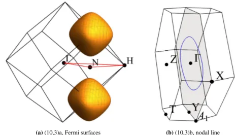
plaquette fluxes [46, 47]. In parallel, O’Brien et al. have used the projective symmetry group approach by Wen [16, 20] to classify the gapless and gapped Z ² spin liquids which occur in a family of elementary 3D Kitaev systems, and have shown that these systems host a variety of different Majorana (semi)metals with characteristic features, such as topological Fermi surfaces, nodal lines and Weyl nodes [35, 36, 48].

Both the thermodynamic results of Nasu and Motome, and the classification of gapless Z 2 spin liquids by O’Brien et al. constitute the starting point for the work which is presented in this thesis. In a first project, we have adapted the quantum Monte Carlo method introduced in Ref. [44] to perform large-scale nu- merical studies on the thermodynamics of elementary 3D Kitaev systems, as they are classified in Ref. [36] (Chapter 4). A second project has extended these quan- tum Monte Carlo studies to a generalized Kitaev system, which shows spin liquid ground states with different kinds of topological order (Chapter 5).

In the remainder of this introductory chapter, we present a brief review on the general theoretical foundation of our work by, first, discussing the role of lattice gauge theories in the realm of quantum spin liquid physics. In particular, we introduce the notion of a Z 2 spin liquid and how it relates to other spin liquid versions. Also, we take a glimpse at the question of stability of spin liquids.

Finally, we comment on where our work is located in the broader field of studies on quantum spin liquids. There is an abundance of literature on the subject [3–

8, 20, 49–51]. The presentation in this chapter is primarily based on Refs. [7, 49–

51].

1.1 Lattice gauge theories

Originally, lattice gauge theories have been developed as discretized versions of gauge theories in quantum field theory, which allow for the study of strongly in- teracting particles beyond perturbative approaches, and have a special relevance for the description of quarks in quantum chromodynamics [52]. It has been soon discovered that there is a natural connection to statistical mechanics, and, in par- ticular, quantum magnets, where systems of spins on lattices can be treated with lattice gauge theories [22].

In the context of quantum spin liquids, the low-temperature description of a

spin system in terms of parton degrees of freedom is usually accompanied by the

emergence of a gauge field on the underlying lattice. Hence, it is possible to use

the corresponding lattice gauge theory to deduce important physical properties of the QSL state, such as the gapless or gapped nature of the gauge excitations, the existence of short-ranged or long-ranged interactions between quasiparticles, and the stability of the QSL state with respect to quantum and thermal fluctuations.

As it turns out, a lot of these fundamental properties can already be extracted from the elementary symmetry of the gauge theory, such as the (continuous) U (1) or the (discrete) Z 2 symmetry. For instance, in Z 2 spin liquids like the Kitaev model, the parton description of the system is usually based on two different ex- citations, namely fermionic spinons, i.e., charge-neutral spin-1/2 quasiparticles, and bosonic visons, which are topological vortex excitations of the Z 2 gauge field [43]. The vison excitations in Z 2 gauge theory are generically gapped. This im- plies that they can only mediate short-ranged interactions between the spinons, which are renormalization-group-irrelevant and therefore do not affect the spin liquid state in the (0 ^th -order) mean-field approximation [20, 49, 53]. In this sense, the Z ² spin liquid is stable to quantum fluctuations.

Following the introduction in the textbook by Wen [49], we use the term gauge theory to denote a theory where more than one label is used to describe the same quantum state. In spin liquids, this redundancy occurs when more than one gauge field configuration describes the same physical state of the system. In this sense, a gauge transformation is a mapping from one “gauge field label” of the same physical state to another such label. Physical quantities are invariant under such gauge transformations, hence, in order to describe the Hilbert space of the system and, for instance, find its ground state, it is necessary to identify the relevant gauge-invariant quantities.

1.1.1 Lattice U (1) gauge theory

An intuitive approach to a number of basic concepts in lattice gauge theory is provided by first looking at the (compact) lattice U (1) gauge theory, which is a discretized version of electromagnetism [7, 49]. Here, the vector potential A translates to discrete field variables A ij , which are defined on the bonds of a three- dimensional cubic lattice, and for which A ij = − A ji . The scalar potential φ, on the other hand, translates to field variables φ i on the lattice sites i. In this setup, physical observables can be defined by the (integer-valued) electric field e ij on the bonds,

e ij = d

dt A ij (t) + φ i (t) − φ j (t),

[A ij , e ij ] = i, (1.1)

1.1. Lattice gauge theories

and the magnetic U (1) flux through the square plaquettes p of the lattice, Φ p = X

hi,ji∈p

A ij , (1.2)

where the notation h i, j i describes the summation over lattice bonds. A simple Hamiltonian for this lattice gauge theory can be formulated as [49]

H ^U(1) = J 2

X

hi,ji

e ² _ij − g X

p

cos(Φ p ), (1.3) where J and g are coupling parameters. This Hamiltonian is periodic with respect to the fields A ij , with periodicity 2π, so the equivalence relation A ij ∼ A ij + 2π defines the compactness of the theory. In addition, H U(1) is compatible with the presence of charges on the lattice sites, which are the eigenvalues of the field- divergence operator

q i = X

j∈nn(i)

e ij , (1.4)

where the summation is over the nearest-neighbor sites of i [7]. The U (1) nature of this lattice gauge theory can be best seen when we go over to the exponentiated flux definition

e ^iΦ

= Y

hi,ji∈p

u ij = Y

hi,ji∈p

e ^iA

. (1.5)

As it is known from electromagnetism, a redundant labelling of the field variables can be introduced in terms of an arbitrary scalar field χ(t). The lattice U (1) gauge transformation is given by

A ij (t) → A ij (t) + χ j (t) − χ i (t),

φ i (t) → φ i (t) + ˙ χ i (t), (1.6) and leaves the Hamiltonian H ^U(1) invariant. Also, the electric field e ij and pla- quette flux variables Φ p are gauge-invariant.

Conceptually, it is insightful to regard the ground state regimes of the Hamil- tonian in Eq. (1.3), which occur in the different coupling limits. For the limit g J, the dominant flux term in the Hamiltonian can be Taylor-expanded as

− g X

p

cos(Φ p ) → g 2

X

p

Φ ² _p + O (Φ ³ _p ), (1.7)

and the exact solution of the theory for all q i = 0 is just standard vacuum elec-

tromagnetism, which can be shown to possess gapless photon excitations [49]. In

this limit, the theory (in 3D) is said to be in the deconfined or Coulomb phase.

In the limit g J, on the other hand, the elementary excitations are loops, which are defined by the nonzero electric field variables e ij on the lattice bonds.

These loops have a finite energy gap, and in the presence of a pair of charges q i = +1, q j = − 1, the electric field generates a potential that grows linearly with the number of bonds between those charges. Hence, the energy that is necessary to separate such a pair of charges diverges for the infinite lattice system. Such a linear potential is called a confining potential, and therefore, the phase is denoted as the confined phase of lattice U (1) gauge theory.

If we go from three to two spatial dimensions, the compact lattice U (1) gauge theory can be shown to always be in the confined phase, because the regime de- fined by g J is destabilized by the occurrence of instanton excitations, which lead to additional interaction terms in the gauge theory, and create a gap for the photons [7, 49, 54].

1.1.2 Lattice Z ² gauge theory

Definition

The lattice Z 2 gauge theory [49–51] can be obtained in a similar way. Here, we start only from the (exponentiated) link variables u ij on a square (or cubic) lattice, as are defined in Eq. (1.5), and restrict them to ± 1. This is equivalent to choosing the vector potential A ij ∈ { 0, π } . Again, we have the relation u ij =

− u ji . If we formulated a Hamiltonian as a direct function of these link variables H = − J P

u ij , it would just be the classical Ising model (which can be seen by replacing u ij = s i s j , with s i/j = ± 1). In this case, every configuration |{ u ij }i would label a different state in the Hilbert space.

In contrast with that, a general d-dimensional lattice Z 2 or Ising gauge theory, here denoted by M dn , takes the product of spins around n-dimensional objects, such as lines (n = 1), plaquettes (n = 2), volumes (n = 3), etc., and formulates a Hamiltonian in terms of these products [50]. In this notation, the lattice Z 2

gauge theory M d1 is the standard d-dimensional Ising Model, and M d2 is the d- dimensional Ising gauge theory, where the most general, classical Hamiltonian is expressed in terms of Z 2 plaquette flux operators W p (see Fig. 1.1),

H Z

,class. = − g X

p

W p , W p = Y

hi,ji∈p

u ij . (1.8)

The definition of W p can be naturally extended to arbitrary closed loops in the

system. In this case, the operator is known as Wilson or Wegner-Wilson loop W l ,

and defines a Z 2 flux ± 1 through the lattice region that is enclosed by the loop.

1.1. Lattice gauge theories

(a) Plaquette flux operator W

and gauge trans- formation operator D

(b) Sign flips to change between degenerate pla- quette flux ground states

Figure 1.1: Lattice Z

gauge theory on the square lattice. Fig. (a) shows the definition of the plaquette flux operators W

and the gauge transformation D

. In Fig. (b), the colored links indicate the sign flips σ

along the vertical (blue) and horizontal axis (red) that have to be performed on the link variables u

, in order to construct the 4-fold degenerate plaquette flux ground states.

In the following, we consider the model M 22 on the (two-dimensional) square lattice. In this lattice model, the configurations |{ u ij }i are a redundant labelling of physical states, and hence, deserve the name gauge configurations. The physical states are, for the square lattice with open boundary conditions, defined by the pla- quette flux states { W p } , which can be seen by defining the gauge transformation [49]

u ⁰ _ij = D i u ij D ⁻¹ _j , (1.9) where the operators D i are arbitrary ± 1-valued functions acting on the lattice sites. A useful explicit definition of D i is provided by introducing the spin flip operator σ ij , which changes the sign of a link variable as u ij → − u ij , and making it act on all nearest neighbors of the site i ¹ [51],

D i = Y

j∈nn(i)

σ ij . (1.10)

Clearly, [W p , D i ] = 0 for all sites i and plaquettes p, so the physical states of the open system can be labelled in a one-to-one manner by the flux states { W p } .

For the square lattice with periodic boundary conditions, things are slightly more complicated. Here, the product of all plaquette flux operators is constrained as

Y

p

W p = 1. (1.11)

1

Adding a term − K P

i

D

to H

yields exactly the Hamiltonian of Kitaev’s Toric Code

model [11].

Therefore, from the 2 ^N plaquette flux states in the periodic 2D square lattice with N sites, only 2 ^N−1 are linearly independent. In the Ising gauge model M 22 , there are, in total, 2 ^N+1 states (equivalence classes under the gauge transformation), which follows from dividing the 2 ^2N gauge configurations |{ u ij }i by 2 ^N−1 (which corresponds to 2 ^N gauge transformations, divided by 2 elements of the Z 2 gauge group). Hence, for each plaquette flux configuration, there are four physical states.

From a gauge configuration |{ u ij }i , the other three states that give the same pla- quette flux configuration can be constructed by

1. flipping the sign of all link variables u ij that cross a defined horizontal line 2. flipping the sign of all link variables u ij that cross a defined vertical line 3. doing both steps 1. and 2.

This is visualized in Fig. 1.1.

Confined and deconfined phase

A quantum version of the lattice Z 2 gauge theory M 22 (and, likewise, for any d- dimensional gauge theory M d2 ) is provided by adding a term to the Hamiltonian that contains the sum over all spin-flip operators σ ij ,

H Z

= − g X

p

W p − t X

ij

σ ij . (1.12)

This extended definition introduces a hopping in terms of the Z ² fluxes, and any state |{ u ij }i is, under H Z

, converted into a highly-entangled superposition state.

At the same time, the Hamiltonian H Z

is gauge-invariant with respect to the transformation in Eq. (1.9) [49].

In close analogy to the lattice U (1) gauge theory, we can now distinguish a deconfined and confined phase for H Z

:

For g t, the ground states of the Hamiltonian are defined by the homoge- neous plaquette flux configuration { W p = 1 } and are, as shown above, four-fold degenerate. The gauge-invariant wavefunction for each such ground state is pro- vided by symmetrizing the corresponding gauge configuration |{ u ij }i over all gauge transformations D i ,

| ψ ₀ ^d i = Y

i

(1 + D i ) |{ u ij }i , (1.13)

and is macroscopically entangled. The four-fold degeneracy of the ground state is

called topological, as it cannot be lifted by any local perturbations to the Hamil-

tonian [49]. One degenerate state can only be converted into another by applying

a number of gauge flip operators σ ij that corresponds to the linear system size L.

1.1. Lattice gauge theories

Flipping a single link variable u ij , on the other hand, creates a pair of (bosonic) Z 2 flux excitations, which are called vortices or visons. The creation of isolated visons is only possible by generating a vison pair, and then applying a non-local string of operators σ ij to separate them – which causes no further energy cost.

Hence, they are non-local excitations. The vison excitations in Z 2 gauge theories are always gapped, and the gap ∆ is of the order g.

This phase is called the Z 2 deconfined phase, and its low-energy properties are determined by the topological degeneracy ( Z 2 topological order) and the existence of non-local, gapped vison excitations.

In contrast, for g t, there is a unique ground state | ψ ^c ₀ i = P

{u

} |{ u ij }i , which seems highly entangled at first sight, but simply corresponds to an Ising state with all spins pointing in the x-direction,

| ψ ^c ₀ i = O

i

|→i i . (1.14)

This can be seen by mapping the link variables u ij to Pauli operators, u ij → σ _ij ^z , and using that the eigenstates |→i , |←i of σ ^x and the eigenstates |↑i , |↓i of σ ^z are related as

|→i = 1

2 ( |↑i + |↓i ),

|←i = 1

2 ( |↑i − |↓i ). (1.15) This phase is the Z 2 confined phase. It doesn’t have a topological order, and the elementary excitations are local, as they can be simply created by applying operators σ _ij ^z to individual lattice bonds.

Ising duality and inverted phase transitions

There is also a well-developed knowledge about the thermodynamics of lattice Z 2

gauge theories. In Ref. [50], Wegner has shown that the lattice Z 2 gauge theories

M dn and M d(d−n) are always connected by a duality relation. This implies that

the partition function Z (and all derived thermodynamic quantities) of a model

at temperature T is related to the partition function of its dual at the temperature

T ^∗ , which is a decreasing function of T . Accordingly, the high-temperature and

low-temperature phase of the dual M d(d−n) are inverted with respect to the original

model M dn . In particular, the three-dimensional lattice Z 2 gauge theory M 32 of the

form given above is the dual of the three-dimensional Ising model, and exhibits a

(continuous) thermal phase transition, which is inverted with respect to the Ising

phase transition [55]. Therefore, it is called an inverted Ising transition.

(a) Ising duality (b) Wegner-Wilson loop

Figure 1.2: Ising duality and Wegner-Wilson loop. Ising gauge theories M

and M

are connected by a duality relation [50], which holds in particular for the three-dimensional Ising model M

and the lattice Ising gauge theory M

(a). Here, the low-temperature deconfined phase of M

is the dual of the Ising paramagnet, and separated from the confined phase by a continuous phase transition (inverted Ising phase transition). For 1 < n < d, this phase transition does not possess a local order parameter. However, both phases can be distinguished by the scaling behavior of the Wegner-Wilson loop W

= Q

hi,ji∈l

u

(b). For the deconfined phase, h W

i scales with the perimeter of the enclosed area, and, for the confined phase, with its area [51].

The phase transition of the d-dimensional Ising model and the corresponding dual lattice gauge theory belong to the same universality class [56–58]. However, Wegner proves that for the lattice Z 2 gauge theory M dn with 1 < n < d, the phase transition deviates from the conventional Ginzburg-Landau paradigm [13–15], in the sense that it does not require a broken symmetry in terms of any local order parameter. For M d2 and d > 2, it instead separates the topologically non-trivial, low-temperature deconfined and a high-temperature confined phase. Instead of a local order parameter, both phases can be distinguished in terms of the average Wegner-Wilson loop h W l i (see Fig. 1.2): In the confined phase, it is expected that h W l i obeys an (extensive) area law in terms of the area A l enclosed by the contour l, such that h W l i ∼ exp( − aA l ), which is a consequence of heavily fluctuating fluxes in this phase. In the deconfined phase, on the other hand, vortex excita- tions are suppressed and h W l i is expected to decay only (subextensively) with the perimeter P l of the enclosed area as h W l i ∼ exp( − bP l ). In correspondence to the scheme of inverted Ising transitions, the deconfined phase, where the plaquettes are ordered, is the dual of the disordered Ising phase, and the (high-temperature) confined phase is the dual of the ordered Ising phase [51].

1.1.3 Emergence of gauge fields in spin liquids

We have seen that the lattice U (1) gauge theory is a discretized version of electro-

magnetism, and contains gapless excitations in the deconfined phase. The bosonic

vortex excitations in lattice Z 2 gauge theory, on the other hand, are always gapped.

1.1. Lattice gauge theories

For both lattice gauge theories, we have distinguished the deconfined and confined phase. At the example of the lattice Z 2 gauge theory, we have seen that the de- confined phase is a non-trivial phase, which is characterized by topological order, non-local excitations and a ground state wavefunction with macroscopic entangle- ment. The question is now how all this knowledge can be used for understanding quantum spin liquids.

As it turns out, lattice gauge theories generically emerge in the description of spin liquids, when the latter are represented using a parton approach. Such an approach can be realized in terms of a slave-boson (projective construction) [26, 59–61] or slave-fermion ansatz [62, 63], and is necessary to enable the treatment of spin liquid models with mean-field methods. This is seen when considering, for example, a Heisenberg model on the two-dimensional square lattice,

H = X

hi,ji

J ij S _i · S _j , (1.16)

which, in the mean-field approximation, is decoupled as H MF = X

hi,ji

J ij ( h S _i i · S _j + S _i · h S _j i − h S _i i · h S _j , i ) . (1.17) Usually, the ground state | ψ MF i of H ^MF can be calculated by choosing an adequate ansatz for h S _i i , such that the self-consistency equation h S _i i = h ψ MF | S _i | ψ MF i is fulfilled [49].

Clearly, such an approach is only well-suited for ordered spin states, where h S _i i is expected to be finite, but not for spin liquids, which are interesting pre- cisely because h S _i i = 0 in the ground state. However, an alternative strategy to perform the mean-field analysis on spin liquids can be pursued by first replacing the spins with parton operators. One (but not the only) possible ansatz is provided by introducing spin-1/2 charge neutral spinon operators f iα (α = 1, 2) as [49, 59]

S _i = 1

2 f _iα ^† σ αβ f iβ , (1.18)

which leads to a Hamiltonian that is quartic in the spinons, H = − X

hi,ji

1

2 J ij f _iα ^† f jα f _jβ ^† f iβ + const. (1.19)

With the transformation in Eq. (1.18), the local Hilbert space of the system is

artificially extended from dimension 2 to 4, which produces unphysical states,

and has to be remedied by introducing a half-filling constraint f _iα ^† f iα = 1 on the

fermions. The (0 ^th order) mean-field approximation is then implemented by

1. replacing the operator f _iα ^† f jα by its ground-state expectation value,

χ ij = h f _iα ^† f jα i , (1.20) and

2. loosening the half-filling constraint, and let it be fulfilled only on aver- age, h f _iα ^† f iα i = 1, which is done by adding the site- and time-dependent Lagrange-multiplier term,

a 0 (i)(f _iα ^† f iα − 1), (1.21) to the Hamiltonian.

Choosing an ansatz (χ _ij , a 0 (i)) for both quantities, the ground-state expectation value χ ij and the Lagrange multiplier a 0 (i), the mean-field Hamiltonian assumes the form

H ⁰ MF = − X

hi,ji

1 2 J ij

f _iα ^† f jα χ _ij + h.c.

− | χ _ij | ² + X

i

a 0 (i)(f _iα ^† f iα − 1), (1.22) and the self-consistency equation is given by χ _ij = h f _iα ^† f jα i [49]. Likewise, the ansatz for the Lagrange multiplier a 0 (i) has to fulfill the relaxed half-filling constraint h f _iα ^† f iα i = 1.

Now, the 0 ^th order mean-field Hamiltonian in Eq. (1.22) describes a system of free fermions, but this description is clearly qualitatively wrong, as the ansatz has changed not only the Hamiltonian, but also the Hilbert space of the Heisenberg model by allowing individual sites to violate the half-filling constraint. Thus, it looks as if nothing was gained from the entire procedure. However, it is possi- ble to fix this issue and recover the original Hilbert space by introducing (mass- less) phase fluctuations (χe ^−iA

, a 0 (i)) around the mean-field state (which can be shown to enforce the half-filling constraint for all sites [49, 59]). In this first-order mean-field approximation, the Hamiltonian becomes

H ¹ MF = X

hi,ji

− J ij

f _iα ^† f jα χ _ij e ^−iA

+ h.c.

+ X

i

a 0 (i)(f _iα ^† f iα − 1), (1.23) and is invariant under the lattice U(1) gauge transformation

A ij → A ij + χ j − χ i ,

f i → f i e ^iχ

. (1.24)

So, instead of a system of free fermions, the Hamiltonian H MF ¹ now describes

fermions, which are coupled to an emergent U (1) gauge field [49]. Notably, it is

1.1. Lattice gauge theories

precisely the introduction of gauge fluctuations which has recovered the original Hilbert space of the system, so it can be concluded that the emergent gauge field is a necessary ingredient for the valid parton description of the spin system (in the words of Wen, the gauge field is required to “glue” the spinons “back together”

[49]). Remarkably, the question if the parton description is only a formal rewriting of the spin system, or if it gives access to physical properties that would otherwise stay unrevealed, now depends on the phase of the emergent gauge field. For the confined phase of the gauge field, the parton description is just a reformulation of the spin system, which does not provide any physical insight, as the system is still fully governed by the fluctuations of spins. In the deconfined phase, on the other hand, the spinons and the emergent gauge field truly behave as independent quasiparticles, and it is exactly this scenario which characterizes the spin liquid state. In this sense, the knowledge about confined and deconfined phases in lattice gauge theories directly translates to the understanding of spin liquids.

There are alternative ways to perform the mean-field approximation for the spinon approach in Eq. (1.18), which essentially distinguish themselves by the pairing channels that are chosen for the spinon operators f iα . All these approaches first lead to a qualitatively wrong 0 ^th order mean-field description of the spin sys- tem, as any such mean-field ansatz artificially expands the Hilbert space and, on a more fundamental level, breaks the local symmetry of the original Hamiltonian.

However, it is always possible to find a global gauge symmetry which the 0 ^th or- der mean-field Hamiltonian still preserves. This global gauge symmetry is called the invariant gauge group (IGG), and it is converted into a local gauge symme- try in the first-order mean-field approximation by introducing IGG-fluctuations.

Generically, it can be shown that a mean-field ansatz which is invariant under the invariant gauge group IGG leads to a low-energy description of the correspond- ing spin liquid in terms of fermionic spinons, which are coupled to an IGG gauge field. The question if the first-order mean-field solution allows for mass terms in the fluctuations then reflects the nature of excitations of the corresponding spin liquid, and, in consequence, its stability [20, 53]:

• The U(1) spin liquid possesses a gapless gauge boson beside further gapped excitations. The U (1) gauge bosons always mediate long-ranged interac- tions between the fermionic spinons. For certain systems, these interactions do not affect the stability of the spin liquid regime, which can be shown with renormalization group methods. Such systems are, due to the power- law decay of correlations between the gauge bosons, called algebraic spin liquids. Generically, however, RG-relevant long-range interactions or the instanton effect makes the U (1) spin liquid unstable.

• In contrast, all bosonic gauge excitations in the Z 2 spin liquid are gapped,

and can only mediate short-ranged interactions. These interactions are gener- ically RG-irrelevant and do not affect the stability of the spin liquid. There- fore, it is also called a rigid spin liquid.

• A rigid spin liquid can also be realized if the invariant gauge group is SU (2), but the SU(2) fluctuations are suppressed by a Chern-Simons term in the underlying action, which is needed if the filled spinon band has a finite Hall conductance [10, 21]. Such chiral spin liquids are quantum spin liquids with broken time-reversal symmetry. They are the spin version of Chern in- sulators [64–68], i.e., systems with a gapped bulk and gapless (chiral) edge states, which are topologically protected by the bulk gap. The existence of such edge modes can be tracked by a topological Z -invariant, the Chern number which is given by the integral of the Berry curvature over the first Brillouin zone.

Parton approaches to spin liquids are not restricted to mean-field treatments, and the emergence of a gauge field is a generic feature of these approaches. In the end, a valid description of the spin system is achieved when the algebra of spin operators is faithfully reproduced by the parton ansatz, which often requires the introduction of additional constraints, in order to reproject the parton system to its physical subspace. We see in Chapter 2 that the Kitaev model, which is in the focus of this thesis, can be solved by a parton ansatz which introduces real (Majorana) fermions as spinons, which are coupled to a Z ² gauge field. In this basis, the system is even exactly solvable and renders the application of mean- field methods obsolete in many situations. However, it is also possible (and, for some purposes, even more insightful) to study the Kitaev model with an ansatz that uses complex fermions [36, 53].

1.2 Thermodynamics of quantum spin liquids

The common understanding of the quantum spin liquid state in an earlier period of

discussion has been focused on the absence of long-range ordering, and the anal-

ogy of this state to classical liquids. According to this point of view, it is natural

to expect that the QSL state is only well defined at exactly T = 0, and for any

finite temperature destabilized by thermal fluctuations. With this understanding, it

is presumed that the spin liquid phase is adiabatically connected to the paramag-

netic gas phase of the spin system, as is the case for classical liquids [44]. But also

from the modern point of view, which defines the QSL phase as a macroscopically

entangled quantum many-body state, one can argue that it might be only realized

for T = 0. Here, it is usually pointed out that any system at finite temperature

shows an extensive (volume law) entanglement, and therefore acquires classical

1.3. Summary

correlations [7]. Hence, it is also expected that a generic QSL state is not protected by a thermal phase transition, and the transition to the high-temperature phase is realized as a smooth crossover.

However, considering that the low-temperature physics of spin liquid systems can be captured in terms of partons coupled to gauge fields, it is the general knowl- edge about lattice gauge theories that provides us with classes of systems which deviate from this generally assumed behavior. Specifically, it can be argued that spin liquids with gapped gauge excitations, such as Z 2 spin liquids, which are sta- ble against quantum fluctuations, are also candidates for a thermally stable phase, which persists up to some finite temperature T c . In this thesis, we discuss that this is indeed the case for Kitaev systems, which are either defined in three spatial dimensions, or which possess a ground state that is topologically protected by the breaking of time-reversal symmetry. In the case of three-dimensional Kitaev Z 2

spin liquids, Wegner’s studies on lattice Z 2 gauge theories even equip us with the universality class of the phase transition. For most 3D Kitaev systems, the spin liquid ground state phase is separated from the paramagnetic state by an inverted Ising phase transition, which is described in terms of loop-like vison excitations.

Later on, we see that the paramagnetic phase is further subdivided into an inter- mediate regime, where the physics is still essentially described by fractionalized degrees of freedom – this phase may also be considered as a proximate Z 2 spin liquid [69] – and the true paramagnetic phase, that is merely a spin gas.

1.3 Summary

Lattice gauge theories are discretized versions of gauge theories from quantum field theory, which are useful for the description of spin systems. They are char- acterized by the symmetry of their underlying gauge transformation as U(1), Z 2

etc., which also determines the gapless or gapped nature of their elementary exci-

tations. Lattice Z ² gauge theories always possess gapped vison excitations. The

three-dimensional lattice Z 2 gauge theory is the dual of the three-dimensional

Ising model, and its deconfinement-confinement transition is inverted with respect

to the Ising phase transition. In quantum spin liquids, lattice gauge theories arise

in the context of the parton description of the spin model. The low-temperature

behavior of spin liquid systems is, in this approach, described by fractionalized

spinon degrees of freedom, which are coupled to an emergent gauge field. Here,

the symmetry of the underlying lattice gauge theory allows for conclusions about

the stability of the spin liquid state.

Chapter 2

Kitaev Model

The Kitaev model is the prototypical example of a quantum spin liquid model that possesses an exact solution. Introduced and solved by Kitaev in his seminal paper of 2006 [27], this particular version of a quantum compass model [70, 71]

has ever since become a research field of vast interest in both theoretical and experimental condensed matter physics [8, 38–43]. The experimental enthusiasm for the model has been triggered in 2009 by Jackeli’s and Khaliullin’s proposal for a real material mechanism that leads to the occurrence of Kitaev interactions in certain Mott insulators with strong spin-orbit coupling, such as Na 2 IrO 3 , Li 2 IrO 3

and α-RuCl 3 [37, 72]. Since then, not only have various experimental groups joined in the race to detect signatures of the quantum spin liquid phase in those Kitaev materials [38, 43], but also, there has been an ongoing search for potential alternative realization mechanisms [73]. A fundamental breakthrough in the hunt for signatures of the spin fractionalization in Kitaev magnets has been the recent measurement of the half-integer thermal quantum Hall effect in α-RuCl 3 [74, 75].

In this chapter, we give a detailed introduction of the Kitaev model and its so-

lution, which is the foundation for our numerical studies on the thermodynamics

of various 2D and 3D Kitaev systems. We start by explaining the solution ansatz

that is used in the original paper by Kitaev [27], which is based on the local trans-

formation of the original spin degrees of freedom to Majorana fermions coupled

to an emergent Z ² gauge field. Here, a close look is given to Lieb’s theorem,

which makes a statement about the ground state configuration of the correspond-

ing gauge-invariant quantity, the Z 2 plaquette flux. Fixing the gauge field to the

ground state plaquette flux configuration, we are able to calculate Majorana band

structures and resolve their topological features, such as the graphene-like Dirac

cones that the Kitaev honeycomb model exhibits at zero temperature. With this

exact solution figured out, we explain how it can be obtained in an alternative way,

namely by a non-local Jordan-Wigner transformation of the spins [76–80]. The

latter becomes important in the context of developing a numerically exact, sign-

problem-free quantum Monte Carlo algorithm for Kitaev systems (Chapter 3). In this first part, the presentation is based on Refs. [27, 77, 78].

After that, we present how the Kitaev model can be extended to lattice systems in three spatial dimensions, and review the Majorana (semi)metals that are found in these systems. Here, the ground state plaquette flux is harder to determine, since most of these systems lack the geometric requirements for the rigorous ap- plicability of Lieb’s theorem. This section is followed by a discussion of the elementary excitations of the Z 2 gauge field, the so-called visons, which have a fundamentally different nature in two and three spatial dimensions. In a section on the thermodynamics of Kitaev systems, we see that the loop-like nature of the vison excitations in 3D is the basis for the occurrence of an inverted Ising phase transition in these systems. The presentation in this part is based in particular on Refs. [36, 44, 50, 51, 81].

We also discuss that Kitaev systems with broken time-reversal symmetry can host topologically non-trivial ground states. In particular, this is the case for non- bipartite Kitaev systems in two spatial dimensions, where the ground state breaks time-reversal symmetry spontaneously. In this context, we introduce a generalized version of the Kitaev model for arbitrary odd-coordinated lattice systems, which can be defined in terms of Γ-matrices [82, 83]. The presentation here relies in particular on Refs. [27, 30, 47, 83].

Finally, we close this chapter by giving a brief overview on the material real- izations of the Kitaev model, which is mainly based on Refs. [37, 38, 73].

2.1 Definition and solution

2.1.1 Spin model and fractionalization

The Kitaev model is defined on three-coordinated lattice systems. It describes spin-1/2 degrees of freedom, which exist on the lattice sites and interact via bond- dependent Ising interactions. The Hamiltonian is given by [27]

H ^Kitaev = X

hi,ji

J γ σ _i ^γ σ ^γ _j , (2.1)

where the σ i are the Pauli matrices and the index γ labels the three subclasses of

x-, y- and z-bonds (Fig. 2.1). For each of these subclasses, the spins interact only

via the respective γ -component. This way, each spin ends up with three compet-

ing interactions, which cannot be satisfied at the same time. This phenomenon is

called exchange frustration. In the classical version of the Kitaev model, where

the SU(2) spins σ i are replaced with O(3) vectors S _i , the exchange frustration

leads to a macroscopically degenerate ground state manifold of the system, which

2.1. Definition and solution

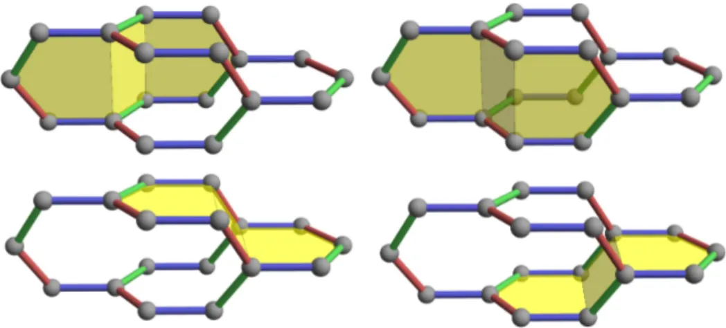
(a) Kitaev honeycomb model (b) Kitaev hyperhoneycomb model

Figure 2.1: Kitaev model on the honeycomb (a) and hyperhoneycomb lattice (b) [27, 34, 36]. The Kitaev model is an exactly solvable quantum spin liquid model, which can be defined on three- coordinated lattices. Spin-1/2 degrees of freedom on the lattice sites interact via bond-dependent Ising interactions − J σ

σ

.

has been shown to be equivalent to the full set of dimer coverings on the under- lying lattice [84]. Here, in the quantum version, the ground state is instead given by a single wave function with macroscopic entanglement, which constitutes a quantum spin liquid.

Local Majorana transformation

The latter can be derived by applying a parton approach to the system, in which the spins are locally transformed to Majorana fermions. For this, each spin operator σ i is replaced by four Majorana fermion operators c i , b ^x _i ,b ^y _i , b ^z _i via [27]

σ ^γ _i = ib ^γ _i c i . (2.2)

The Majorana operators b ^γ _i , c i fulfill the canonical commutation relations { b ^α _i , b ^β _j } = 2δ ij δ αβ ,

{ c i , c j } = 2δ ij ,

{ c i , b j } = 0, (2.3)

and reproduce two of the fundamental relations of the Pauli matrices, (σ ^γ ) ² = 1,

(σ ^γ ) ^† = σ ^γ . (2.4)

However, reproducing the full spin algebra,

[σ ^α , σ ^β ] = 2i αβγ σ ^γ ,

{ σ ^α , σ ^β } = 2δ αβ , (2.5)

requires the introduction of an additional constraint to the Majorana operators.

The reason behind this is a change in dimensionality that is typical for parton approaches: The local Hilbert space in the Majorana basis is 4-dimensional (=

( √

2) ⁴ ), while in the spin basis, it only has dimension 2. The transformation in Eq. (2.2) thus artificially increases the local Hilbert space of each spin. Only a subspace reproduces the spin algebra, though, and can therefore be considered as physical. This physical subspace is obtained by introducing a Z 2 gauge transfor- mation [27],

D i = b ^x _i b ^y _i b ^z _i c i , (2.6) and consists of all states | ξ i which are Z ² gauge-invariant, i.e., for which

D i | ξ i = | ξ i . (2.7)

The transformation in Eq. (2.2) replaces the Ising terms in the Hamiltonian ac- cording to σ _i ^γ σ _j ^γ = − i(ib ^γ _i b ^γ _j )c i c j , i.e., it reveals an interaction that is quadratic in the Majorana fermions c i . The operators b ^γ in the interaction term can, on the other hand, be combined to bond operators [27],

ˆ

u ^γ _ij = ib ^γ _i b ^γ _j , (2.8)

with u ˆ ji = − u ˆ ij . They commute with each other and with the Hamiltonian and have eigenvalues ± 1. Therefore, they can be replaced by their eigenvalues u ij in the Hamiltonian, which then assumes the form [27]

H ( { u ij } ) = 1 4

X

i,j

iA ij c i c j , (2.9)

with the matrix A defined by

A ij = 2J ^γ u ^γ _ij , (2.10)

for connected sites i,j (otherwise, A ij = 0).

Physically, we now have the paradigmatic scenario for quantum spin liquids,

where the original spin degrees of freedom are fractionalized, and the fraction-

alized version of the system includes the description in terms of a lattice gauge

theory. Here, the spinon degrees of freedom are given by the non-interacting Ma-

jorana fermions c i , which are coupled to the emergent Z 2 gauge field { u ij = ± 1 }

on the lattice bonds (Fig. 2.2). Since the bond operators u ˆ ij commute with H ,

the Z 2 gauge field is static. Hence, if a configuration { u ij } is fixed, the model is

exactly solvable by diagonalizing the Majorana fermion system, i.e., the complex

tight-binding matrix iA in Eq. (2.9). Since iA is Hermitian, its eigenvalues come

in (real) pairs ± λ . These are the single-particle energy levels of the Majorana

fermions.

2.1. Definition and solution

Figure 2.2: Kitaev honeycomb model in the Majorana basis. In this representation, the original spin degrees of freedom are fractionalized to (itinerant) Majorana fermions situated on the lattice sites (black), which are coupled to an emergent (static) Z

gauge field on the bonds (red, green, blue) [27].

Vacuum state

The Majorana basis is, however, unsuited to determine a ground state (vacuum state) of the system, because here, the creation and annihilation of a particle are the same, c ^† = c. Therefore, the system has to be rewritten in terms of com- plex (Dirac) fermions a ^† _λ . Such a canonical diagonal description is achieved by a pairwise recombination of the Majoranas. For this, we first apply a basis transfor- mation of the operators c i to normal modes [27],

(b ⁰ ₁ , b ⁰⁰ ₁ , ..., b ⁰ _m , b ⁰⁰ _m ) = (c 1 , c 2 , ..., c 2m−1 , c 2m )Q, (2.11) where Q is a transformation matrix consisting of the real (imaginary) parts of the eigenvectors of iA in their odd (even) columns. The matrix A and the eigenvalues i of iA are related with the transformation matrix Q by

A = Q















0 1

− 1 0 . ..

0 m

− m 0















Q ^T . (2.12)

After this basis transformation, the spinless fermionic operators a λ , a ^† _λ are intro- duced as [27]

a ^† _λ = (b ⁰ _λ − ib ⁰⁰ _λ )/2,

a λ = (b ⁰ _λ + ib ⁰⁰ _λ )/2. (2.13)

Figure 2.3: Elementary plaquette of size | p | = 6 in the honeycomb lattice [27]. Taking the product of the Z

gauge variables u

along the plaquette yields the gauge-invariant Z

plaquette flux W

= Q

( − iu

) = ± 1.

Thus, the N Majorana operators are mapped to N/2 spinless fermions a ^† _λ , and the final diagonal representation of the Kitaev Hamiltonian in a fixed Z 2 gauge field configuration { u ij } reads

H ( { u ij } ) =

N/2

X

λ=1

λ

a ^† _λ a λ − 1 2

. (2.14)

The ground state energy of the Majoranas in the gauge field configuration { u ij } is now obtained simply by setting the fermionic counting operators n ˆ λ = a ^† _λ a λ = 0 for all λ,

E ( { u ij } ) = − 1 2

N/2

X

λ=1

λ . (2.15)

2.1.2 Lieb’s Theorem

Z 2 plaquette flux

As a result of the described transformations, the problem of obtaining the ground state of the full spin system is reduced to finding the Z ² gauge field configuration { u ij } which minimizes the energy (2.15). The bond operators u ˆ ij are clearly not gauge-invariant, because they change their sign under any gauge transformation D i that is applied to one of their adjacent sites i,

D i u ˆ ij = − u ˆ ij , (2.16)

2.1. Definition and solution

Thus, it is necessary to find the corresponding gauge-invariant quantity for the Z 2

gauge field { u ij } , which is expected to be associated with some physical observ- able.

Reminding ourselves of the general formulation of the lattice Z 2 gauge theory in Sec. 1.1.2, we find that this gauge-invariant quantity is already well known as the plaquette flux, which has been written in terms of the operator W p , Eq. (1.8).

There is an interesting mathematical-physics perspective on this quantity, which relates it to the energy spectrum of arbitrary tight-binding electron Hamiltonians with nearest-neighbor hopping t ij = | t ij | e ^iφ

. As it turns out, for a fixed con- figuration of coupling parameters t ij , this spectrum only depends on the phase variables φ ij through the flux Φ around the elementary plaquettes p, i.e., the loops of shortest length of the corresponding lattice [85–87]. This flux Φ is, in the most general version, defined by

e ^iΦ = Q

hi,ji∈p t ij

Q

hi,ji∈p | t ij | , (2.17)

and corresponds to the plaquette flux that is defined in Sec. 1.1.2 for the lattice Z ² gauge theory M d2 . In Kitaev systems, the plaquette flux operator e ^iΦ in Eq. (2.17) is usually also denoted by W p . We obtain it by taking the product of the Kitaev bond terms around the plaquettes, where, as a standard, we multiply the bond terms in a clockwise manner. Thus, in the spin and Majorana basis, the Z 2 pla- quette flux operator reads [27]

W p = Y

hi,ji

∈p

σ _i ^γ σ ^γ _j

= Y

hi,ji

∈p

( − iu ^γ _ij ). (2.18)

The eigenvalues of W p are ± 1 for plaquettes with even and ± i for plaquettes with odd length, and the (clock- or counterclockwise) direction of measurement only affects the sign of the odd-length plaquettes. We use the convention that an eigenvalue W p = +1 = e ⁱ⁰ is identified with the absence of a Z 2 plaquette flux ( = 0-flux), while an eigenvalue ˆ − 1 = e ^iπ signifies the presence of a Z 2 plaquette flux ( = ˆ π-flux) ¹ .

W p is clearly invariant under the gauge transformation D i , since, for any pla- quette, the latter always changes the sign of two Z 2 gauge variables u ij within that plaquette. But this is not all. W p also commutes with the Hamiltonian H ( { u ij } ), and therefore provides an extensive set of conserved quantities { W p } for the Ki- taev model. In consequence, the Hilbert space H of the system is divided into

1

In the remainder of this thesis, we often use the convention to denote the flux operator eigen-

value W

also by the name “plaquette flux”.

Z 2 gauge-invariant subspaces H {W

} , which are given by the eigenspaces of the plaquette flux operators W p , and called flux sectors,

H = M

{W

}

H {W

} . (2.19)

Thus, in the sense of the general gauge theory definition that is given in Chapter 1, the Z ² gauge configurations { u ij } are redundant labellings of the Z ² flux config- urations { W p } , and likewise, different gauge sectors H {u

} of the Hilbert space provide a redundant description of the physical flux sectors.

Ground state flux sector

Having this gauge-invariant quantity W p defined, the remaining problem is to find the plaquette flux configuration { W p } which gives a minimal energy. This prob- lem has been the subject of numerous studies in mathematical physics [85–87]

(Appendix A.1). The most striking result is a theorem by Lieb [86], which states that the flux ground state for an arbitrary half-filled band system of hopping elec- trons and a bipartite lattice with (at least) semi-periodicity is determined by the elementary plaquette length | p | of the lattice. If | p | mod 4 = 0 (e.g., in the square lattice), the energy of the system is minimized by a plaquette flux Φ = π. Quite remarkably, this means that the presence of a magnetic flux lowers the energy, a phenomenon which can only occur for systems with high electron density. On the other hand, if | p | mod 4 = 2 (e.g., in the honeycomb lattice), the ground state plaquette flux is Φ = 0. A general formula for the plaquette flux is thus given by

Φ = π( | p | − 2)

2 . (2.20)

However, Lieb’s theorem is not universally applicable. In non-bipartite lattice systems, we have seen that the odd-length elementary plaquettes have direction- dependent loop operator eigenvalues W p = ± i. Here, the nature of the flux ground state is fundamentally different from bipartite systems, since there is no energetic selection of one distinguished flux state. Instead, the two possible flux states are connected by time-reversal symmetry, and the ground state spontaneously breaks TR symmetry by selecting either of the two states for all plaquettes.

Also for bipartite lattice systems, Lieb’s theorem is only rigorously proven for

systems with a specific geometric condition. The whole lattice (i.e. the sites and

bonds, along with the configuration of coupling constants J γ ), and the individual

plaquettes, for which the flux is minimized, have to be invariant under reflection

symmetry. Moreover, the corresponding mirror plane must not cut through any

vertices of the lattice. This condition is fulfilled for the honeycomb lattice. Going