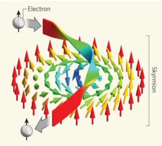
Skyrmions and Monopoles in Chiral Magnets & Correlated Heterostructures

(1)

Skyrmions and Monopoles in Chiral Magnets

&

Correlated Heterostructures

Inaugural-Dissertation zur

Erlangung des Doktorgrades

der Mathematisch-Naturwissentschaftlichen Fakultät der Universität zu Köln

vorgelegt von

Christoph Sch¨utte

aus Dormagen

K¨oln 2014

(2)

Berichterstatter: Prof. Dr. Achim Rosch (Gutachter)

Priv.-Doz. Dr. Ralf Bulla

Tag der m¨undlichen Pr¨ufung: 17. April 2014

(3)

Abstract

The first part of this thesis is called “Skyrmions and Monopoles in Chiral Magnets” and concerned with topological spin textures in chiral magnets.

The second part, “Correlated Heterostructures”, studies layered, strongly correlated devices within the framework of dynamical mean-field theory.

In magnets without inversion symmetry, so called chiral magnets, weak spin-orbit coupling leads to the formation of smooth twisted magnetic struc- tures with a long period. Recently, a new magnetic phase of a lattice of topo- logically stable whirl-lines was discovered. In the first chapter we introduce the concept of a such a whirling texture and briefly mention its occurrence in other areas of physics. In chapters 2 we review the Ginzburg-Landau theory for chiral magnetic structures describing their equilibrium properties followed by a description of a numerical minimisation technique to explore the mean-field configuration of the free energy functional. In chapter 3 we review the Langevin description for a system at finite temperature and con- centrate on especially on the description of magnetic systems. The describe how a numerical integration of the equations of motion, a stochastically dif- ferential equation, can be achieved to compute ensemble-averaged quantities.

Chapter 4 we present the discovery of emergent magnetic monopoles as the

driving mechanism behind topological phase transitions from the Skyrmion

lattice into topologically trivial phases. We describe how a Skyrmion lattice

unwinds due to the motion of magnetic monopoles in the system as seen both

in experiment and numerical simulations. We investigate how the energetics

of and forces between monopoles and antimonopoles influence their creation

rate and dynamics. In chapter 5 we turn to the dynamical properties of single

Skyrmions in ferromagnetic backgrounds. In a first approach we study ana-

lytically the fluctuations around the mean-field configuration and determine

the spectrum of the bound states, the scattering solutions and their phase

shifts and coupling mechanism to the collective Skyrmion coordinate. By

integrating out the fluctuations we discover a strongly frequency-dependent

e↵ective mass for the collective Skyrmion coordinate. We approach the same

question from a di↵erent angle in the second part of the chapter. Here we

(4)

start from numerical simulations of the stochastic Landau-Lifshitz-Gilbert equation and determine the coefficients of the e↵ective equations of motion from a statistical analysis of the collective coordinate fluctuations. We find a strongly frequency-dependent e↵ective mass and a new peculiar damping mechanism proportional to the acceleration of the Skyrmion that we call

‘gyro-damping’.

The second part of this thesis explores the interface e↵ects in strongly correlated heterostructures. Multilayered heterostructures in the nano sized realm (also known as multilayered nanostructures) are the most common electronic devices. A classic multilayered nanostructure is a tunnel junction consisting of two metallic leads connected by a “weak link”, often a conven- tional band insulator. The connection between the two leads is thus governed by inherently quantum mechanical e↵ects. We begin with an introduction to model Hamiltonians, in particular the Hubbard and the single impurity An- derson model. The second chapter describes the static mean-field treatment of anti-ferromagnetic order in the Hubbard model. Chapter 3 introduces the reader to the dynamical mean-field theory (DMFT) and describes extensions of the DMFT to system with antiferromagnetic order. The DMFT maps the lattice problem onto an e↵ective impurity problem. In chapter 4 we review how the single impurity Anderson model can be solved using the numerical renormalisation group (NRG). The generalisation of DMFT to inhomoge- nous, layered systems is given in chapter 5 including the e↵ects of long-range Coulomb interactions on the Hartree level. Here we also outline our generali- sation of the inhomogenous DMFT to systems with antiferromagnetic order.

In chapter 6 we derive expressions for the layer-resolved optical conductivity and the Hall conductivity. We apply the former to the Mott-Band-Mott het- erostructure where we study the transport properties of the two-dimensional metallic state at the interface where we find a rich temperature dependence.

In chapter 7 we turn to the question how the transmission amplitude through

a Mott insulator in a linear potential depends on temperature.

(5)

Kurzzusammenfassung

Der erste Teil dieser Arbeit “Skyrmionen und Monopole in chiralen Mag- neten” besch¨aftigt sich mit topologischen Magnetisierungs-Texturen in chi- ralen Magneten. Der zweite Teil, “Korrelierte Heterostrukturen”, untersucht Korrelations-E↵ekte an Grenzschichten zwischen verschiedenen Materialien in Heterostrukturen.

In chiralen Magneten bilden sich auf Grund schwacher Spin-Bahn- Wech- selwirkung verdrillte, magnetische Konfigurationen aus, wie beispielsweise Helizes mit einer langen Periodenl¨ange. K¨ urzlich wurde eine neue magnetis- che Texture bestehend aus topologisch stabilen “Wirbel-Linien”, sogenan- nten Skyrmionen, entdeckt. In dieser Arbeit untersuchen wir den topol- ogischen Mechanismus, der zu einer Zerst¨orung des Skyrmionen-Gitters in Phasen¨ ubergangen f¨ uhrt. Wir untersuchen dar¨ uber hinaus die dynamischen Eigenschaften von getriebenen Skyrmionen eingebettet in einen ferromag- netischen Hintergrund.

Im zweiten Teil dieser Arbeit besch¨aftigen wir uns mit Heterostrukturen

in Rahmen der dynamischen Molekularfeld Theorie. Speziell untersuchen

wir Grenzschichte↵ekte von stark-korrelierten, geschichteten Systemen. Wir

berechnen schicht-aufgel¨oste Transportkoeffizienten und Tunnelwahrschein-

lichkeiten durch Mott-Barrieren.

(6)

Introduction

Nowadays, topology has firmly established itself as a vital tool in every physicists’

mathematical arsenal and all modern theories contain topological ideas of some sort or another. The applications range from the gauge theories in particle physics, where monopoles, instantons and solitons describe non-perturbative excitations, to the space time topology of general relativity. Also in condensed matter physics topology has proven itself indispensable. Noteworthy occurrences include topological insulators, the quantum Hall e↵ect and defects in ordered media. The unique role topology plays in physics established its status as a universal and ubiquitous paradigm.

The links between the very old subject of physics and the much younger

¹

mathe- matical discipline of topology date back to the 19th century. The earliest connection occurs in the work of Kirchho↵, 1847, who uses graph-theoretical methods to solve the equations for a general electric network [51]. But also mathematicians have found in- teresting applications of topological ideas to physical problems. For instance, Gauss noted that Ampere’s law may be understood as the linking number between two curves and iterated his confidence that this is only one of many topological ideas to be eventually discovered in the field of physics [37]. One of the most common applications of topology in present-day condensed matter physics may be homotopy theory which is vital for the description of topological solitons.

Topological solitons are classical solutions of the Lagrangian equations of motion homotopically distinct from the vacuum solution. Often this occurs when the surface on which the boundary condition is specified has a non-trivial homotopy group. Such solutions can be interpreted as particles of the theory which owe their stability against (quantum-) fluctuations to their non-trivial topology. Historically, the first example of a topological soliton model for an elementary particle was the Skyrmion. The Skyrmion emerged from the Yukawa model, a field theory for the three types of spinless pions. Skyrme believed that the particles in a nucleus were moving in a non- linear, classical pion medium [93]. Symmetry arguments lead to a particular form of the Lagrangian which allowed topologically stable soliton solutions of the classical field equations, distinct from the vacuum. These solutions could then be understood as baryons.

As mathematical objects Skyrmions have also gained importance in solid state physics. Here a noteworthy example is a two-dimensional electron gas exhibiting the integer quantum Hall e↵ect. The low energy theory of such as system has the structure of a quantum ferromagnet with elementary excitations given by dressed particles

1Listing was the first to use the term ‘Topologie’ in 1836 [61].

(10)

whose local magnetisation wraps the Bloch sphere once when exploring the two- dimensional plane. In analogy to the mathematical structure of Skyrme’s solutions these excitations are referred to as Skyrmions. Another occurrence of Skyrmions in solid state physics was discovered in 2009 when a Skyrmion lattice was shown to exist in the chiral magnet MnSi as the stable phase in a region of the magnetic phase diagram [72]. Here similar to a vortex lattice in type-II superconductors, the magnetic phase is characterised by a hexagonal lattice of magnetic whirls arranged in a plane perpendicular to an applied magnetic field and translationally invariant along the direction of the field. The magnetisation throughout the unit cell remains finite, wraps the unit sphere once and can thus be described by an integer-valued topological index, i.e. a winding number. The discovery of the Skyrmion lattice has spurred great interest in these whirling spin textures and raised hopes that they might find application in spintronic devices and future information storage technologies.

In this part of the thesis, we study the dynamical properties of Skyrmions in chiral magnets. We begin with a general introduction to Skyrmions and a brief sum- mary of their discovery in chiral magnets in chapter 1. In the following we outline the Ginzburg-Landau theory for magnetic systems in chapter 2 and the Langevin approach to magnetic systems at finite temperature in chapter 3. The non-trivial topology of Skrymions has important implications for the destruction of the Skyrmion lattice. For instance, due to the conservation of topological charge phase transitions from the Skyrmion lattice into a topologically trivial phase necessarily lead to the ap- pearance of magnetic point defects in the system since the destruction of Skyrmions changes the winding number of the system. In accordance with topological con- straints these defects exhibit properties characteristic of magnetic monopoles and we thus refer to them as “emergent magnetic monopoles”. Chapter 4 describes the exper- imental discovery and analyses their energetics and dynamics through micro-magnetic simulations and numerical minimisation of the free energy functional.

The study of the e↵ective dynamics of single Skyrmion excitations in the fer- romagnetic background is important both from the point of view of fundamental research and possible applications in spintronic devices. In chapter 5 we analyse the fluctuation spectrum around the classical solution of the Lagrangian equations of motion in the single Skyrmion sector by explicitly calculating both the scattering wave functions and internal modes of the Skyrmion. A perturbative expansion in the fluctuations yields a fluctuation-induced inertia term. In section 5.2 we extract the e↵ective equations of motion for a Skyrmion from the statistical analysis of its di↵u- sive motion and study its dynamics when driven by time-dependent electric currents and magnetic field gradients.

4

(11)

Chapter 1 Skyrmions

In the original sense of the word, a ‘Skyrmion’ is a topological soliton solution known to occur in a non-linear field theory for interacting pions originally conceived by the nuclear physicist Tony Skyrme [93]. In a more permissive interpretation of the word Skyrmions, as mathematical objects, have found versatile application in a variety of di↵erent areas in physics. In this chapter we briefly review the historic origin of the Skyrmion and define the generalised concept that is nowadays understood as a

‘Skyrmion’. We outline previous applications in di↵erent fields of physics and then forward to 2009 to give a concise account of the discovery of the Skyrmion lattice phase in the chiral magnet MnSi.

1.1 What is a Skyrmion?

In 1961 before the advent of quantum chromodynamics (QCD) the nuclear physicist T.H.R. Skyrme conjectured that the interior of a nucleus is dominated by a medium formed from three pion fields [93]. He introduced the Skyrme model, a non-linear sigma model, with the intention to describe baryons as the quantised soliton solu- tions of a field theory which involves only bosonic degrees of freedom. The model is understood as an intermediate between the traditional models which represent the nucleons as point particles interacting through a potential, and a complete description based on quarks and gluons [4]. The pion fields ⇡ = (⇡

1

, ⇡

2

, ⇡

3

) are combined into a SU(2)-valued field

U (x) = p

1 ⇡(x) · ⇡(x) 1 + i⇡(x) · , (1.1) where is the vector of Pauli matrices and we have suppressed a possible time dependence of the fields. For static fields the energy in the Skyrme model is given by

E = Z

d

³

r

✓ 1

2 Tr(R

i

R

i

) 1

16 Tr([R

i

, R

j

][R

i

, R

j

])

◆ , (1.2)

where we have introduced an associated current R

i

= (@

i

U )U

^†

and [ · , · ] denotes the

commutator. The vacuum is represented by U (x) = 1. For the energy to be finite, U

must approach a constant at infinity [65]. The energy is invariant under translations

(14)

and rotations in R

³

and also under the transformation U ! AU A

^†

with A 2 SU (2), one may thus choose U(r ! 1 ) = 1. E↵ectively, due to this boundary condition space is then topologically (but not metrically) compactified to S

³

, and since the group manifold of SU (2) is also S

³

, U defines a map from S

³

to S

³

. The structure of the homotopically distinct maps U is given by the third homotopy group ⇡

₃

( S

³

) which happens to be isomorphic to Z . The space of all maps U : S

³

! S

³

decomposes into distinct subsets characterised by an integer-valued topological charge B = R

d

³

r B with the topological charge density B given by

B = 1

24⇡

²

✏

ijk

Tr(R

i

R

j

R

k

) . (1.3) The minimal energy solutions for each B are called Skyrmions and their energy is identified with their mass and B with the Baryon number of the nucleus. The B = 1 Skyrmion has the spherically symmetric hedgehog form [65]

U(x) = exp(if(r)ˆ r · ) , (1.4) where f (r) is a radial profile function obeying an ordinary di↵erential equation with the boundary conditions f(0) = ⇡ and f(r ! 1 ) = 0.

Skyrmions in their original sense are therefore smooth, topologically stable ex- tremal field configurations which are trivial at spatial infinity and have a finite en- ergy. They are defined by surjective mappings into the order parameter space S

³

and characterised by a non-trivial topological charge B. Since the nth homotopy group of S

ⁿ

is isomorphic to Z for any n 1, a more permissive definition of “Skyrmion” is given by

A skyrmion is a smooth field configuration defined by a topologically non-trivial, surjective mapping from a base manifold M into the order parameter space T ' S

ⁿ

, trivial on the surface of M and characterised by a finite integer-valued topological charge.

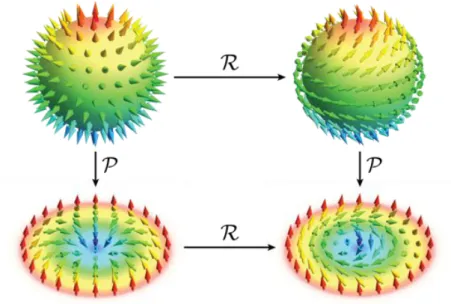
Fig. 1.1 shows the construction recipe for M = R

²

and T = S

²

. We start with the identity map, ˆ ⌦(ˆ x) = ˆ x, with ˆ x 2 S

²

which can be visualised as a hedgehog configuration (c.f. Fig. 1.1, top left). The stereographic projection P maps the sphere onto the two-dimensional plane, P (ˆ x) 2 R

²

and thus a Skyrmion configuration is given by the mapping ˆ M : R

²

! S

²

, ˆ M : r 7! ⌦ ˆ P

¹

(r). The corresponding topological charge W is given by R

d

²

r W where we have defined the topological charge density W as

W = 1

8⇡ M ˆ · (@

_x

M ˆ ⇥ @

_y

M ˆ ) . (1.5) W counts the number of times the mapping ˆ M sweeps out the target manifold S

²

. From the construction recipe above it is obvious that for the Skyrmion (Fig. 1.1 lower left) W = 1. The color code has been chose such that arrows pointing to the north pole are plotted in red and those to the south pole as blue and the equator in green.

A chiral, non-inversion symmetric Skyrmion can be constructed if the hedgehog is additionally ‘combed’ by performing a ⇡/2 rotation R about the ˆ z-axis in order parameter space (Fig. 1.1 top right), ˆ N : r 7! R ⌦ ˆ P

¹

(r). R is a linear map on S

²

8

(15)

Figure 1.1: Construction recipes for the non-chiral and chiral skyrmion from the hedgehog configuration. R denotes a rotation about the ˆ z-axis acting in order pa- rameter space and P the stereographic projection.

and therefore W = 1 for this configuration as well. These later, chiral Skyrmions (Fig. 1.1 lower right) will be the main focus of this thesis. In contrast to a Skyrmion, a vortex does not sweep out the whole sphere. For example a vortex configuration is given by the map V : R

²

! S

²

, V : r 7! ˆ e (r), where ˆ e = ( sin( ), cos( ), 0)

^T

in polar coordinates (r, ). The vortex only sweeps out the equator, is singular at r = 0 and has a non-trivial winding for r ! 1 .

1.2 Skyrmions in other areas of physics

Within this generalised understanding Skyrmions have found versatile application in many di↵erent fields of physics. Here we only mention a few.

In 1985 Klebanov proposed the possibility of a Skyrmion crystal [52]. A phe- nomenological application of this kind of a solution could be a neutron crystal, which may exist under high pressure inside neutron stars [108]. The theory might resolve puzzles concerning discrepancies about the maximum mass of stable neutron stars be- tween observations and predictions by more traditional equation of state descriptions [47].

Liquid crystals are states of matter which show characteristics of those of a con- ventional liquid and those of a solid crystal. Many interesting ordering phenomena have been reported in these systems where the local order parameter is describe by a director field ( a field of headless vectors) rather than a vector field [110]. Among these the blue phases which have a regular three-dimensional cubic structure of de- fects with lattice periods of several hundred nanometers are particularly interesting.

Here so-called 2⇡ disclinations are singular line defects where the 2⇡ indicates that

(16)

the director rotates a full 360 as the singular line is encircled. These singular defect configurations are unstable towards a non-singular configuration that di↵ers from its original one only in the immediate neighborhood of the formerly singular line. For the 2⇡ disclinations these non-singular configurations are given by Skyrmion config- urations of directors in n = 2. Recently it was shown theoretically [34], with the aid of numerical methods, that a highly chiral nematic liquid crystal can accommodate a quasi-two-dimensional Skyrmion lattice as a thermodynamically stable state, when it is confined to a thin film between two parallel surfaces.

Skyrmions were predicted to occur in quantum Hall systems close to the Landau level filling fraction ⌫ = 1 for sufficiently small Zeeman splitting gµ

B

B (compared to the the cyclotron gap !

c

= eB/mc) [97]. The incompressible ground state of a two-dimensional electron gas at this filling fraction is ferromagnetic. For sufficiently small g < g

c

the charged excitations of the system were argued to be Skyrmions where their winding number is related to the charge ⌫e of the Skyrmion. The equivalence of physical charge and topological charge in the system is a consquence of the quantum Hall e↵ect and is responsible for the dominating role of Skyrmions in determining many physical properties [28]. Brey and collaborators proposed that ground state close to ⌫ = 1 is a crystal of charged Skyrmions [11]. Nuclear magnetic resonance measurements in GaAs provided only indirect evidence [3, 92].

Topologically, skyrmions are equivalent to certain magnetic bubbles (cylindrical domains) in ferromagnetic thin films, which were extensively explored in the 1970s for data storage applications [64]. In ferromagnets where long-range order is frustrated due to long-range dipole-dipole interactions a wealth of di↵erent magnetic patterns can be seen, such as domain walls, vortices and periodic stripes. In Ref. [112] Lorentz transmission electron microscopy (LTEM) was used to show that a magnetic field applied perpendicular to a thin film of hexaferrite turns the periodic stripe domain state into a periodic, hexagonal lattice of chiral Skyrmion bubbles (c.f. Fig 1.1 lower right). In contrast to other materials however where the inversion symmetry of the atomic unit cell is broken, in hexaferrite the helicity of the Skyrmion is not fixed by crystal structure, but represent a Z

2

degree of freedom and a random distribution of di↵erent helicities in the lattice can be observed. Here even helicity reversals within a single Skyrmion where observed. Note that the helicity is independent of the winding number which can be seen from the fact that one may smoothly deform helicities into one another.

Bogdanov and collaborators studied the mean-field theory of easy-axis ferromag- nets with chiral spin-orbit interactions. They argued that in certain parameter regimes a mixed state with a finite density of Skyrmions much like the vortex lattice in type II superconductors becomes the thermodynamically stable phase [10]. Al- though the stability analysis was carried out in the circular unit cell approximation the Skyrmion lattice was predicted to be hexagonal [10]. Here the presence of easy- axis anisotropy turned out to be a necessary ingredient for the stabilisation of the mixed phase within the mean-field treatment. Also they assumed the magnetization vector to be homogeneous along the z-axis [9].

10

(17)

1.3 Discovery of the Skyrmion lattice in MnSi

In 2009 M¨ uhlbauer et al. reported the discovery of a Skyrmion lattice phase in the chiral magnet MnSi by a small angle neutron scattering study (SANS). Although in this section we concentrate on MnSi as the first chiral magnet the spontaneous for- mation of this phase of whirling magnetisation has been observed in, the Skyrmion lattice phase has since then been discovered in many other compounds as well. In 2010 the same group discovered a Skyrmion lattice phase in the doped semiconductor Fe

1 x

Co

x

Si [73, 114]. The Skyrmion lattice phase in this material was also later con- firmed by real-space images using Lorentz transmission electron microscopy (Lorentz TEM) [114]. Since then the Skyrmion lattice has been observed in a variety of di↵er- ent materials both as a bulk phase as well as in thin films. Appendix A gives a more elaborate description of the material properties and the magnetic phase diagram of various materials the phase has been observed in. Here we only want to mention that the electronic properties of this set of compounds is very diverse: Among these are metals, insulators, semi-conductors and also a multi-ferroic material. This show that the Skyrmion lattice is not a peculiarity of MnSi but rather a general phenomenon in this class of materials.

The unifying property for all of these materials is that they crystallise in the so-called B20 structure. The symmetry transformations are described by the space group P 2

1

3 with a cubic Bravais lattice [38]. With only 12 symmetry operations this space group is among the smallest compatible with the cubic lattice crystal system.

The point symmetry at the component sites is C

3

, the cyclic group of 3-fold 2⇡/3 rotations about an appropriate [111] axis. The nonsymmorphic group P 2

1

3 contains in addition 3 screw rotations which involve 2-fold rotations about one of the three [100] axis followed by an appropriate non-primitive translation (0,

¹₂

,

¹₂

). Most notably the list of symmetry transformations does not include the inversion. The lack of inversion symmetry has profound consequences for the Ginzburg-Landau free energy description of these materials and for the symmetry constraints on the magnetic configuration that the materials can show. Materials with non-inversion symmetric atomic unit-cells can support non-inversion symmetric magnetic structures. There are other mechanisms by which Skyrmion lattice phase can be stabilised. We will return to this point at the end of this chapter. Although we concentrate prodominantly on MnSi in this chapter, the magnetic phases of MnSi are generic for chiral magnets.

Particularly the phase diagram Fig. 1.2b can be seen as a generic phase diagram for B20 compounds that order helimagnetically.

The primitive cell of manganese silicide (MnSi) contains four pairs of the 2 com- ponent formula units Mn and Si located at (u, u, u), (

¹₂

+ u,

¹₂

u, u), ( ¯

¹₂

u, u, ¯

¹₂

+ u), and (¯ u,

¹₂

+u,

¹₂

u) with u

Mn

= 0.138 and u

Si

= 0.845. MnSi is an itinerant ferromag- net with a fluctuating magnetic moment of 0.4 µ

B

and a saturated moment of 2.2 µ

B

per manganese atom. Before the discovery of the skyrmion lattice phase, it already

attracted attention due to a high pressure anomaly: Although described very well

by Fermi-liquid theory at ambient pressure, MnSi shows a non-Fermi liquid phase

above a critical pressure of p

c

⇠ 14.6 kbar with the temperature dependence of the

resistivity given by T

^3/2

[81, 79]. In addition in the pressure region 12 kbar 20 kbar

(18)

Si T

a c

b

(a) The atomic unit cell comprising four formula units of T Si with T = Mn.

The atoms are located at (u, u, u), (

¹₂

+ u,

¹₂

u, u), ¯ (

¹₂

u, u, ¯

¹₂

+u), and (¯ u,

¹₂

+ u,

¹₂

u) with u

_Mn

= 0.138 and u

_Si

= 0.845.

(b) Magnetic phase diagram of MnSi. For B = 0, helimagnetic order develops be- low T

_c

= 29.5 k. Above B

_c2

the mate- rial field polarises. For intermediate field values the conical phase develops with the Skyrmion lattice phase (A-phase) as a small phase pocket inset in a specific temperature and field range. Taken from Ref. [72].

Figure 1.2

a state of partial magnetic order was encountered in neutron scattering experiments [80].

At ambient pressure and zero applied magnetic field, MnSi develops magnetic or- der below a transition temperature T

c

= 29.5K that is the result of three hierarchical energy scales. The strongest scale is the ferromagnetic exchange favoring a uniform spin polarisation (spin alignment). The lack of inversion symmetry of the cubic B20 crystal structure results in chiral spin-orbit interactions, which may be described by the rotationally invariant Dzyaloshinsky Moriya (DM) interaction favoring canted spin configurations [22, 69]. The DM interaction originates from relativistic e↵ects, i.e. spin orbit coupling

SO

⇠ 10

²

, and is the lowest order chiral spin-orbit interac- tion [2, 74, 83]. In addition there are very weak crystalline field interactions which break the rotational symmetry and align the ordering wave vector of the magnetic structures along the [111] axes [83].

Magnetic phases of MnSi

The magnetic phase diagram of MnSi, Fig. 1.2b, shows four distinct magnetic phases:

a helical phase, a conical phase, a field-polarized phase and the previously mentioned skyrmion lattice phase (for historical reasons referred to as the “A-phase” in the diagram). In the following we briefly describe the magnetic order in each of these.

12

(19)

Figure 1.3: In the helical phase the magnetisation winds around the propagation vector q. The magnetization vectors stand perpendicular on q. Red arrows point into the paper, blue arrows out of it while green arrows lie in the plane of the paper.

Figure 1.4: In the conical phase the spiral propagation vector q aligns parallel to the applied magnetic field B. The magnetization winds around the q similar to the helical phase, however here the magentic moments also tilt towards the propagation vector giving the configuration a uniform magnetisation component along B. Red arrows point into the paper, blue arrows out of it while green arrows lie in the plane of the paper.

Helical phase

Cooling the system at zero or only small applied magnetic field below the critical temperature T

c

⇠ 29 K a phase transition to the helical phase is encountered. In this phase the magnetization winds around an axis parallel to the spiral propagation vector q as shown in Fig. 1.3 with the local magnetic moment M perpendicular to q. The period of the helix,

h

= 2⇡/ | q | is controlled by the competition of the ferromagnetic exchange with the chiral spin-orbit coupling. The weakness of the spin-orbit interaction leads to a wavelength

h

⇠ 190˚ A which is large as compared with the lattice constant, a ⇠ 4.56˚ A. This large separation of length scales results in an efficient decoupling of the magnetic and atomic structures. The direction of propagation ˆ q = q/ | q | is determined by tiny crystal field anisotropies. Therefore, the alignment of the helical spin spiral along the cubic space diagonal [111] is weak and is only fourth power in the small spin-orbit coupling,

⁴_SO

. The decoupling from the underlying atomic structure results in an extremely coherent helical phase with a huge correlation length of 10

⁴

˚ A as reported in this neutron scattering study [59]. While the paramagnetic to helical transition is expected to be second order on a mean-field level, interactions between the helimagnetic fluctuations were theoretically predicted to give rise to important corrections. Indeed it was recently shown that a Brazovskii-type scenario is realized where an abundance of strongly interacting fluctuation distributed uniformly over a sphere in momentum space drives the transition first order [48].

Conical phase

Setting out in the helical phase one finds a phase change upon increasing the applied

magnetic field above B

c1

⇠ 0.1 T. The stronger magnetic field allows for a net

reduction in free energy by building up a uniform magnetic moment in the direction

of the applied field. While for high magnetic fields above B

c2

⇠ 0.6 T the DM

interaction can be completely neglected and the magnetic configuration completely

(20)

(a) In the skyrmion lattice phase the magnetic stucture forms a hexagonal lattice of anti-skyrmions in the plane perpendicular to the applied magnetic field. The lattice constant is given by 2

_h

/ p

3. The state posses a trans- lational invariance along the field magnetic field direction and should therefore be visualised as an ordered arrange- ment of whirling tubes. Here we show only one layer.

(b) Typical SANS intensities for the SkX phase. Red (blue) cor- responds to high (low) intensity.

The color scale is logarithmic to enhance small features. See main text for details.

polarizes, there is an intermediate field range where the magnetization winds both around a spiral propagation vector q parallel to B and in addition possesses a uniform magnetization in the direction of B as the the magnetisation vectors tilt towards

ˆ

q = ˆ B. The phase is referred to as the concial phase and is despicted in Fig. 1.4.

On general grounds a crossover between the helical and the conical phase is expected where the ordering wave vector q rotates continously from the helical [111] direction towards the direction of the applied field. If applied along special high symmetry axis one may encounter a second order phase transition however. The angle between the propagation vector q and the local magnetization M is smooth function of the applied magnetic field B and decreases to zero for B > B

c2

.

Skyrmion lattice phase

A first order phase transition separates a tiny pocket in the magnetic phase diagram close to T

c

at finite magnetic field from the surrounding conical phase. This region, termed for historical reasons “A-phase”, has a hexagonal lattice of anti-skyrmions perpendicular to the applied magnetic field as its ground state. An illustration of the skyrmion lattice is despicted in Fig. 1.5a. The configuration possesses a translational invariance along the direction of the applied magnetic field. The magnetisation con- figuration should therefore be imagined as an ordered arrangement of whirling tubes similar to the flux lattice in a type II superconductor. Fig. 1.5a shows only a single layer. The magnetic configuration can be approximated by a superposition of three helices with their propagation vectors lying in a plane perpendicular to the applied magnetic field and relative angles of 120 plus a uniform magnetic moment antiparal- lel to the applied field. The relative phases are aligned such that the magnetization in the center of the skyrmion points antiparallel to B. The lattice constant is therefore

14

(21)

given by 2

h

/ p

3. The large lattice constant ensures an efficient decoupling of the magnetic structure from the underlying atomic lattice and allows for the orientation towards the applied field. The orientation of the hexagonal lattice within the plane however is determined by crystal field anisotropies. For a magnetic field in the [001]

direction, for instance, one of the three q vectors pins weakly in the [110] direction of the atomic crystal. The building blocks of the lattice are referred to as anti -skyrmions as their their winding number per magnetic unit cell

W = 1 4⇡

Z

UC

M ˆ ⇣

@

x

M ˆ ⇥ @

y

M ˆ ⌘

(1.6) is quantized to -1. Here ˆ M = M/ | M | and the integration is taken over the two- dimensional magnetic unit cell, which contains exactly one “knot”.

The experimental technique used by M¨ uhlbauer et al. was small angle neutron scattering (SANS). Neutron scattering is an ideal tool for the study of magnetic order in bulk phases as neutrons predominantly scatter from the magnetic structure in a solid-state system due to their magnetic moment. The lack of an electric charge allows them to penetrate deep into the system under investigation. The neutrons scatter elastically due to the interaction of their spin with the nuclei and unpaired electrons of the magnetic atoms in the sample and the scattered neutrons are recorded by detectors placed behind the sample. The Fourier modes in the magnetic order are recorded as Bragg peaks in reciprocal space. A more detailed description of SANS can be found in Appendix B. The Skyrmion lattice can be approximated by three helices with their ordering wavevectors in a plane normal to the applied magnetic field and relative angles of 120 . In a typical neutron scattering experiment the incoming neutron beam is perpendicular to the applied magnetic field. In such a setup not all of the 6 reflection spots (two per helix at +q and q) can be seen simultaneously.

The setup chosen by M¨ uhlbauer et al. aligned the incoming beam parallel to the applied field. This setup is much more advantageous and allows to record all 6 spots at the same time, c.f. Fig. 1.5b.

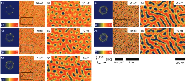
Other experimental techniques were also able to prove the existence of the Skyrmion lattice. In recent years powerful real-space imaging techniques have been modified and applied to chiral magnetic systems which allow for a direct visualization of the spatial magnetization configuration. The advantage of such methods is that not only a single spin texture, but also the crystallization and melting process during phase conversions can be observed. Fig. 1.6a shows images of the Skyrmion lattice phase in a thin film of Fe

0.5

Co

0.5

Si recorded by Lorentz transmission elctron microscopy (LTEM). LTEM is a modification of traditional electron microscopy in which the Lorentz forces between the electrons in a beam and the sample are utilised to gen- erate images which allow for the real-space observation of the magnetic structure of materials. The drawback of LTEM is that samples have to be electron transparent and therefore the technique can only be applied to thin films. Also LTEM images only the in-plane component of the magnetisation.

Real-space images of the surface of bulk materials can be recorded using the mag-

netic field microscopy (MFM). MFM images forces between the surface of a sample

and the magnetic stray field of a cantilever tip coated with a ferromagnetic film. The

total force acting on the cantilever is inferred from small changes in its resonance

(22)

(a) Lorentz TEM images of the Skyrmion lattice in Fe

_0.5

Co

_0.5

Si. Taken from Ref. [113].

(b) MFM images of Skyrmions from the surface of bulk Fe

_0.5

Co

_0.5

Si. Taken from Ref. [67].

Figure 1.6

frequency. It is complementary to LTEM in the sense that it is only sensitive to the out-of-plane component of the magnetisation. Fig. 1.6b shows MFM images of Skyrmions from the surface of bulk Fe

0.5

Co

0.5

Si. Red (blue) color indicates an out- of-plane component of the magnetisation that is anti-parallel (parallel) to the line of sight. For more information about real-space imaging techniques, see Appendix B.

Other physical quantities also show signatures in the Skyrmion lattice phase. For instance the magnetic AC suscpetibility shows a sudden drop to a lower when entering the Skyrmion phase from the conical phase by increasing the applied field.

It then rises exceeding the value in the conical phase before entering the conical phase once again for higher magnetic fields [101]. A more dramatic e↵ect can be seen in measurements of the Hall e↵ect in MnSi. Here due to the unique topology of the Skyrmion lattice an additional top hat contribution to the Hall signal can be seen in the Skyrmion lattice phase [85]. Chapter 4 contains an elaborate discussion of the physical e↵ect and the experimental measurements.

Ever since the original discovery of Skyrmions in chiral magnets in 2009, many exciting developments have deepened our unstanding of these fascinating structures.

Here we mention only a few. Neubauer et al. showed that the topological properties of the Skyrmion lattice lead to additional contribution to the Hall signal, called the topological Hall e↵ect[75]. Everschor et al. analyzed the spin-transfer e↵ects result- ing from an electric current driven through a Skyrmion lattice, and, in particular, focussed on the current-induced rotation of the magnetic texture by an angle in such a setup [26]. Schulz and collaborators have shown that the forces acting on conduction electrons moving through a Skyrmion lattice can be accounted for by the introduction of emergent (fictious) electromagnetic fields. This o↵ered fundamental insights into the connection between the emergent and real electrodynamics of skyrmions in chiral magnets [88]. Iwasaki et al. showed in a numerical study that a single skyrmion can be created by an electric current in a simple constricted geometry comprising a plate-shaped specimen of suitable size and geometry [45]. In experimental realisation of Skyrmion creation however with a di↵erent mechanism was reported by Romming and collaborators in 2013. They showed that on an ultrathin magnetic film in which individual skyrmions can be written and deleted in a controlled fashion with local spin-polarized currents from a scanning tunneling microscope [86]. There have been

16

(23)

many more interesting and noteworthy publications which we cannot mention here

and without question there will be many more.

(24)

18

(25)

Part I

Methods

(26)

(27)

Chapter 2 Ginzburg-Landau theory for Helimagnets

In the vicinity of a second order phase transition, the correlation length of a system diverges. This indicates that the properties near the critical point are independent of the microscopic details. Many universal system properties can therefore be described by phenomenological theories which reduce the redundancy in the system description greatly. A phenomenological theory for contiuum phase transitions is given by the so called Ginzburg-Landau theory. Based on Landau’s theory of second-order phase transitions [57], Ginzburg and Landau expanded the free energy of a superconductor in terms of an order parameter , which is nonzero in the ordered phase and vanishes above the transition temperature T

c

thus laying the foundation for what became one of the most successfull and widely used theories in condensed matter physics.

In this chapter we will give an introduction to Ginzburg-Landau theory for the description of magnetic systems. In section 2.1 we will start with a very general description of the structure of this theory and then apply it to the special case of helimagnets in section 2.2.1.

2.1 Theory of continuum phase transitions

The microscopic origin of magnetism in metals involves the quantum mechanical

treatment of spinful, itinerant electrons and is highly complicated and material de-

pendent. The full theory allows to answer the question which materials will exhibit

ferromagnetism. However assuming that a given system shows such behaviour, a

microscopic theory is neither necessary nor desirable to describe for instance the dis-

appearance of magnetic order due to thermal fluctuations. The degrees of freedom

which describe the transition are long wave-length collective spin excitations with

typical length scales much in excess of the lattice constant. Therefore an e↵ective de-

scribtion can be achieved by coarse-graining the system and modelling the magnetic

order by the average magnetization of a large number of spins. The average magne-

tization is then a smooth function on the the length scale of the lattice constant and

one arrives at a continuum theory.

(28)

Figure 2.1: The order parameter depends on temperature and other external param- eters. In second-order phase transitions the order parameter is a continous function of the system temperature T and vanishes above a crititical temperature T

c

.

The state of many condensed matter systems can be described by the appearance of a certain order in the system or the absence of the same. The order parameter is a concept which seeks to quantify the “amount of order” present in the system.

Examples of order parameters are, for instance: magnetization M (ferromagnets), polarization P (ferroelectrics), distortions (structural transitions) and the complex order parameter field in superconducting systems.

Typically at high temperatures the system is disordered as the state is chosen by minimization of the corresponding thermodynamic potential, i.e. Gibbs free energy.

For large T the deciding factor is the entropy of the system, which it seeks to maximize hence favouring disordered system. Lowering the temperature the importance of the entropy is diminished and the systems seeks to optimize its internal energy arranging its degrees of freedom in an ordered fashion.

Therefore the order parameter ⌘ of the system depends on temperature and other external parameters. For now we will assume that the state of the system can be described by a spatially homogenous order parameter. It is non-zero in the ordered phase of the system and vanishes upon increasing the system temperature above the critical temperature T

c

. For second order phase transitions this happens in a continous fashion, Fig. 2.1. The state of the system and in particular the value of the order parameter ⌘ is determined by the condition that the (Gibbs) free energy G is minimized. The free energy is related to the systems partition function Z

Z = e

^G

= Z

D ⌘e

^F[⌘]

, (2.1)

where F [⌘] is the free energy functional.

Due to the smallness of ⌘ close to the critical point T

c

the free energy functional F [⌘] can be expanded in a power series

F [⌘] = F

0

+ ↵⌘ + ⌘

²

+ ⌘

³

+ ⌘

⁴

+ . . . (2.2) It should be noted that this expansion can only involve terms, which are compatible with the symmetries of the microscopic Hamiltonian. The coefficients are functions of the external system parameters. In the mean-fied approximation one simply looks at

22

(29)

Figure 2.2: Sketched dependence of the free energy F [⌘] on the parameters ↵ and . For ↵ = 0 (no external field) the order parameter vanishes above the transition temperature, i.e. (T > T

c

) 0.

the stationary points of the free energy functional, neglecting any fluctuations around this point,

G ⇠ min

⌘

F [⌘] = F [⌘

0

]. (2.3)

For a vanishing linear term ⇠ ↵ the free energy functional develops a minimum at

⌘ = 0 for T > T

c

; the order parameter vanishes above the critical temperature. The quadratic term must obey the conditions

(T ) < 0, for T > T

_c

(T ) > 0, for T < T

c

(2.4) If the expansion of the free energy is truncated at 4th order the thermodynamic stability of the system is ensured, i.e. a diverging order parameter ⌘ is prevented, only if the prefactor of the quartic term is positive, > 0. The dependence of F [⌘] is sketched in Fig. 2.2.

The Gaussian fluctuations around the mean field ⌘

₀

are the leading order correc- tion to the mean field result

G ⇠ F [⌘

0

] + 1 2 ln det

✓

₂

F

⌘ ⌘

◆

⌘0

(2.5) As we will see later these fluctuations can play a decisive role as to what phase the system will actually realize.

2.2 Ginzburg-Landau theory for magnetic systems

For a ferromagnetic system, such as iron, the order parameter is given by the mag- netization M. Below the critical temperature T

_c

, the Curie temperature, the system spontaneously orders characterized by a finite magnetization M, the thermal average of the microscopic magnetic moments. The magnetization is the conjugate, thermo- dynamic variable to the applied magnetic field H. Fixing the direction of H = H e ˆ

z

one finds that for temperatures T < T

c

the regime H > 0 and H < 0 is separated by a line of phase transitions, which ends at T = T

c

at the critical point C, see Fig. 2.3.

The system may be brought from the one regime to the other either by choosing

a discontinous path which crosses the phase boundary (path A) or continously by

driving it around the critical point, T > T

c

(path B).

(30)

Figure 2.3: Phase diagram for a ferromagnet. Here the surface of the equation of state is shown in the space of the conjugate variables, magnetization M and external magnetic field H, and temperature T . For any two states in the state space a con- necting, continous path may be found that avoids the line of phase transition, H = 0 and 0  T < T

c

, by going around the critical point C.

2.2.1 Inversion-symmetric magnetic systems

In the absence of an applied magnetic field the Hamiltonian of typical ferromagnetic system is invariant under

1. spatial inversion, r ! r

⁰

= r 2. time-reversal, t ! t

⁰

= t

In addition in the presence of a magnetic field H it possesses the symmetry M ! M if H ! H. As can be seen in Fig. 2.3 the magnetization M is small in the immediate vicinity of the Curie point C and the correlation length ⇣ diverges. Therefore it is possible to expand the free energy functional F [M] in terms of M and r M. The above list of transformations poses a minimal symmetry requirement that each term in the expansion has to fulfil. Assuming the validity of these claims the expansion of the free energy functional F [M] assumes the form

F [M] = Z

d

³

r ⇥

H

j

M

j

+ r

0

M

_j²

+ U M

_j⁴

+ J (@

i

M

j

)

²

+ . . . ⇤

. (2.6)

Appropriate phenomenological parameters r

₀

, U and J must be chosen for the par- ticular microscopic system. J parametrizes the ferromagnetic exchange: a positive J describes the tendency of neighbouring magnetic moments to align parallel to each other by penalizing spatially modulated order parameter configurations. As already mentioned in section 2.1 the stability of the system requires U > 0. Condition 2.4 constraints the temperature dependence of r

0

. In order to have a finite (vanishing) magnetization for T < T

c

(T > T

c

) r

0

should be negative (positive) below (above) the Curie temperature T

c

. Linearizing the temperature the dependence of r

0

around T

c

one finds

r

0

(T ) = ↵(T T

c

) + . . . (2.7) with a positive constant, ↵ > 0.

For T < T

c

, H the free energy functional F [M] is minimised by spatially homoge- nous configuration M(r) = M

0

. The ferromagnetic exchange term proportional to J

24

(31)

vanishes. The functional Eq. 2.6 is rotationally invariant in this case and the direction of M

0

is spontaneously chosen. The magnitude of M

0

is fixed by minimising the free energy functional

| M

0

| =

r r

0

2U . (2.8)

As for T > T

c

r

0

changes sign and assumes positive values, the square root becomes imaginary and signals a vanishing of the magnetisation, M

0

= 0. For T < T

c

| M

0

| assumes finite, positive values.

2.2.2 Non-inversion-symmetric magnetic systems

In certain materials so-called chiral magnets the atomic unit cell lacks inversion sym- metry. Appendix A describe 4 exemplary materials which belong to this class. The absence of this symmetry transformation relaxes the symmetry requirements imposed on the free energy functional F [M] and allows for additional terms to appear in the expansion: terms with an odd number of spatial derivatives transform odd under inversion symmetry. Of these previously forbidden terms that may now appear in Eq. 2.6 the Dzyaloshinskii-Moriya (DM) interaction with only a single spatial deriva- tive is the most important contribution.

Z

d

³

r 2D M · ( r ⇥ M) (2.9)

Originally derived on phenomenological grounds by Dzyaloshinskii [22] to explain the appearance of weak antiferromagnetism in materials such as Fe

₂

O

₃

and the carbonates of Mn and Co, Moryia went on to explain the origin of this term as a combination of superexchange interaction and spin-orbit interaction [69]. Thereby the coupling constant D scales linearly in the spin-orbit coupling, D ⇠

^SO

.

Canted magnetization configurations minimize the DM interaction term. The competition with the ferromagnetic exchange interaction leads to the appearance of helical order in the system characterized by an ordering wave vector q = q q, where ˆ the magnetization winds around an axis ˆ q. The pitch q of this helix is determined by the relative strength of the coupling constants D and J.

q = D

J (2.10)

The spin-orbit coupling for the materials we are interested (Appendix A) is small,

SO

⇠ 10

²

. This leads to a small DM interaction and a very large periodicity of the magnetic structures, often making the magnetic unit cell orders of magnitude larger than the atomic unit cell. One finds for the periodicity ⇠

mag

of the magnetic structure

⇠

mag

⇠ q

¹

⇠ D

¹

⇠

SO¹

(2.11)

As spatial derivatives are inversely proportional to the typical length scale over which

the magnetization rotates r ⇠ ⇠

SO

, terms with higher orders of spatial derivatives

are suppressed by the weakness of the spin-orbit coupling

SO

.

(32)

Nevertheless the appearance of terms O(

³_SO

) has important consequences. The presence of higher order terms in the spin-orbit coupling due to crystal field anisotropies breaks the rotational symmetry of the free energy functional F [M] and allows the or- dering wave vector q to choose a preferred orientation ( h 111 i in the case of MnSi, see Appendix A).

2.3 Numerical minimisation of the Ginzburg-Landau functional

The mean-field configurations of the magnetisation can be studied by numerical min- imisation of an appropriately discretised Ginzburg-Landau functional. For the study of phases with a translational invariance a discretisation in momentum space is advan- tageous. For helimagnets a characteristic length scale is defined by the ratio between the ferromagnetic exchange J and the DM interaction D which in term defines a characterisitc momentum, Eq. 2.10. A discretisation of the Functional in terms of q and higher-order moments gives even for a small number of minimisation parameters accurate results. However we will be predominantly interested in mean-field configu- rations which lack translational invariance. In this case better results are achieved if one discretises in real-space. The free-energy functional for a helimagnet up to order

2SO

is given by F [M] =

Z d

³

r ⇥

r

0

M

²

+ J ( r M)

²

+ 2D M · ( r ⇥ M) + U M

⁴

H · M ⇤

. (2.12) It turns out that the number of parameters in the above functional can be reduced by an appropriate rescaling of the length, magnetisation, magnetic field and energy units. By the rescaling

r ! D J r H !

s U

✓ J D

◆

3

H

M ! r U J

D

²

M (2.13)

the free energy functional F [M], Eq. 2.12, can be brought to the form [72]

F [M] = Z

d

³

r ⇥

˜

r

0

M

²

+ ( r M)

²

+ M · ( r ⇥ M) + M

⁴

H · M ⇤

, (2.14) with the rescaled ˜ r

0

=

_D^J2

r

0

and the new energy unit =

^JD_U

. From the above expression we see that the only parameters determining the physics in the Ginzburg- Landau regime are r

0

and H. A discretisation in real-space of the above expression can be achieved when the continous variable r 2 R

³

is replaced with a grid r

ijk

= iaˆ e

_x

+jaˆ e

_y

+kaˆ e

_z

with i, j, k 2 N and a the discretisation constant. The magnetisation

26

(33)

density M will be replaced by the average magnetisation m

ijk

in a single cell with volume a

³

, m

ijk

. In order to keep the energy of the discretised system finite in the limit a ! 0 one has to rescale the magnetisation according to

Z

d

³

r M(r)

⁴

! X

ijk

a

³

M

⁴_ijk

=

^!

X

ijk

m

⁴_ijk

. (2.15)

where M

ijk

= M(r

ijk

). From the above consideration follows that m

ijk

= a

^3/4

M

ijk

. With the same reasoning one finds for the magnetic field h

ijk

= a

^9/4

H(r

ijk

) and for ¯ r

0

= a

^3/2

˜ r

0

. Finding the mean-field configuration of a system parametrised by (r

0

, U, J, D, B) therefore involves two steps. First one rescales the system according to Eq. 2.14 and finds ˜ r

0

. Then a discretisation parameter a is chosen small enough so that the discretised model approximates the continuum model accurately enough and the parameters b and ¯ r

0

of the discretised system are calculated. A numerical minimisation yields a discretised magnetisation configuration which can be translated back to the original model with the above relations.

The discretisation of the model involves the discretisation of the di↵erential oper- ators in the expression for the free energy. After partial integration the ferromagnetic exchange term and its discrete approximation are given by

Z

d

³

r M r

²

M ⇡ a

^1/2

X

ijk

(m

i+1jk

+ m

i 1jk

) · m

ijk

(m

ij+1k

+ m

ij 1k

) · m

ijk

(m

_ijk+1

+ m

_ijk ₁

) · m

_ijk

+ 6m

²_ijk

. (2.16) Similarly the approximation for the DM interaction term assumes the form

Z

d

³

r M · ( r ⇥ M) ⇡ a

^1/2

X

ijk

m

ijk

⇥ m

i+1jk

· ˆ e

x

+ m

ijk

⇥ m

ij+1k

· ˆ e

y

+ m

ijk

⇥ m

ijk+1

· e ˆ

z

. (2.17)

In summary the discretised model is given by f[m] = X

ijk

⇥ (¯ r

0

+ 6/a

^1/2

)m

²_ijk

+ m

⁴_ijk

h

ijk

· m

ijk

a

^1/2

(m

i+1jk

+ m

i 1jk

) · m

ijk

a

^1/2

(m

ij+1k

+ m

ij 1k

) · m

ijk

a

^1/2

(m

ijk+1

+ m

ijk 1

) · m

ijk

a

^1/2

m

ijk

⇥ m

i+1jk

· ˆ e

x

a

^1/2

m

ijk

⇥ m

ij+1k

· e ˆ

y

a

^1/2

m

ijk

⇥ m

ijk+1

· e ˆ

z

⇤ (2.18) For a continuum model discretised on a N ⇥ N ⇥ N grid the above expression is a function of 3N

³

optimisation parameters. An mean-field magnetisation configu- ration can be calculated on a computer using numerical minimisation algorithms.

The conjugate gradient method (CG) is a standard algorithm for the minimisation

of quadratic functions of the form || A · x b ||

²

with the dimensionality of x so large

that a direct calculation is too time-consuming. At the minimum x

^⇤

the gradient

vanishes, r f(x) = 2A

^T

(A · x b) = 0. CG therefore calculates an approximate

solution of the equation ˜ A · x = ˜ b with ˜ A = A

^T

A and ˜ b = A

^T

b. The conjugate

(34)

0 0.05 0.1 0.15 0.2 0.25 Bz

-1.3 -1.28 -1.26 -1.24

E ^λ=1.0

λ=1.1 λ=1.2 λ=1.3 λ=1.4 λ=1.5 λ=1.6 λ=1.7 λ=1.8 λ=1.9 λ=2.0

(a) Energy density E of a discretised he- lix as a function of the applied field B

_z

for various discretisations . For larger they quickly converge to the continuum solution.

1 2 3 4 5

λ -1.27

-1.26 -1.25 -1.24

E

(b) Energy density of a helix at B

_z

= 0 as a function of the discretisation . The approximate energy converges quadrati- cally in agains the exact solution of the continuum model (red dashed line).

Figure 2.4

gradient method has been generalised (non-linear conjugate gradient method) to non- linear optimisation problems. The generalisation may work if the non-linear function is approximately quadratic near the mininum, which is always the case if the function is twice di↵erentiable at the minimum. Over the years a number of di↵erent optimi- sation strategies for non-linear functions have been developed - all based on the CG [31]. For the numerical optimisation of the free energy functional above we use the Fletcher-Reeves variant of the non-linear CG algorithm as implemented in the GSL (GNU Scientific Library). A more detailed account of the algorithm can be found in Appendix C. It should be noted though that the CG method finds local minima - it is not guaranteed to find the global minimum of the functional.

The lattice discretisation a can be used to control how accurately the discretised model approximates the continuum model. As an example we calculate the mean- field configuration of a system with ¯ r

0

= 2 and small magnetic field h. For these parameters the system is in the helical phase and we therefore initialise the system by writing a single period of a helix with the ordering vector q pointing along the x- direction into a system of size 10 ⇥ 1 ⇥ 1 with periodic boundary conditions in the x-, y- and z-direction. Note that due to the translational invariance of the configuration in the y- and z-direction it suffices to choose 1 for N

y

and N

z

. For the discretised system on a lattice the pitch of the helix is given by tan(q) =

^D_J

= a with a the lattice discretisation. The parameter is therefore related to a via a = tan(2⇡/10 ).

Fig. 2.4a shows the energy density E after convergence of the minimisation algorithm as a function of B

_z

for various discretisations . The solutions are seen to quickly converge towards an asymptotic solution for larger s. Fig. 2.4a shows the energy density of the approximation for B

_z

= 0 as a function of the parameter . The solutions converge quadratically in against the energy of the exact solution for the continuum model (red dashed line).

28

(35)

0 0.12 0.25 0.396 0.5 0.75

B

_z

-2 -1.8 -1.6 -1.4 -1.2 -1

E

_hel

E

_skyr

E

_pol

Figure 2.5: Mean-field phase diagram of a 2D helimagnet at T = 0.

2.4 First applications

Magnetic phase diagram of 2D helimagnet

We calculate the magnetic phase diagram (in mean-field approximation) of the two- dimensional helimagnet (in the x-y plane) for ¯ r

0

= 1 and the magnetic field h applied perpendicular to the system, i.e. h = hˆ e

z

. We discretise the system on a 100 ⇥ 100 ⇥ 1-grid with periodic boundary conditions in the x- and y- direction. The local minimum the minimisation algorithm converges to is determined by the initial position in the parameter space, i.e. the initial magnetisation configuration. The only way to determine reliably the actual phase the system will exhibit is to start the algorithm in all possible choices, let it converge and then compare the final free energy densities. The phase with the lowest free energy density is the stable phase of the system. For a two-dimensional helimagnet there are three competing ordered phases:

a helical phase, the Skyrmion lattice phase and the field-polarised phase. Fig. 2.5 shows the free energy density of the converged solutions for the three phases as a function of the applied magnetic field B

z

. For fields in the range 0  B

z

< 0.12 ⌘ B

c1

the helical phase has the lowest energy. At B

z

⇡ 0.12 the free energy density of the helical and the SkX phase become degenerate and for 0.12  B

z

< 0.4 ⌘ B

c2

the SkX phase has the minimal free energy. Above B

z

> 0.4 the system is field- polarised. These results are in qualitative agreement with Monte Carlo results for two-dimensional helimagnetic systems [19].

Skyrmions and Monopoles in Chiral Magnets & Correlated Heterostructures