Collective charge excitations and the metal-insulator transition in the square lattice Hubbard-Coulomb model
Maksim Ulybyshev,1,*Christopher Winterowd,2,†and Savvas Zafeiropoulos3,4,‡
1Institut für Theoretische Physik, Universität Regensburg, 93053 Regensburg, Germany
2University of Kent, School of Physical Sciences, Canterbury CT2 7NH, United Kingdom
3Jefferson Laboratory, 12000 Jefferson Avenue, Newport News, Virginia 23606, USA
4Department of Physics, College of William and Mary, Williamsburg, Virginia 23187-8795, USA (Received 19 September 2017; published 9 November 2017)
In this article, we discuss the nontrivial collective charge excitations (plasmons) of the extended square lattice Hubbard model. Using a fully nonperturbative approach, we employ the hybrid Monte Carlo algorithm to simulate the system at half-filling. A modified Backus-Gilbert method is introduced to obtain the spectral functions via numerical analytic continuation. We directly compute the single-particle density of states which demonstrates the formation of Hubbard bands in the strongly correlated phase. The momentum-resolved charge susceptibility also is computed on the basis of the Euclidean charge-density-density correlator. In agreement with previous extended dynamical mean-field theory studies, we find that, at high strength of the electron-electron interaction, the plasmon dispersion develops two branches.
DOI:10.1103/PhysRevB.96.205115 I. INTRODUCTION
The square lattice Hubbard model has been the focus of intense theoretical research due to its simplicity and the fact that it demonstrates many of the phenomena that are associated with strongly correlated electrons [1]. Furthermore, it is be- lieved that, in some sense, the physics of the high-temperature superconductors can be captured with the Hubbard model [2].
The Mott-Hubbard metal-insulator transition (MIT) [3], the formation of a pseudogap [4,5], and the formation of Hubbard bands [6,7] are all examples of strongly correlated behavior that are expected to appear in the Hubbard model.
In the case of the unfrustrated Hubbard model on the square lattice, it is believed that strong long-range antiferromagnetic fluctuations shift the MIT towards zero on-site coupling as the temperature is decreased towards zero [8]. Furthermore, these spin fluctuations evolve from being Slater-like at weak-lto- intermediate coupling to Heisenberg-like at strong coupling.
More recent studies have extended the interactions in the Hubbard model beyond the on-site term and have included nonlocal correlations. These studies are related closely with the development of extended dynamical mean-field theory (EDMFT) [9,10] along with the EDMFT+GW approach [11] whereGWrefers to the approximation of the self-energy by the first-order graph in which there appears one fermion line (G) and one screened interaction line (W) [12]. Among other phenomena, the inclusion of a long-range Coulomb interaction allows one to study collective charge excitations of the theory. These excitations, known as plasmons, can be accessed via the charge susceptibilityχρ(q,ω) which measures the system’s response to a scalar potentialA0(q,ω). Using the dual-boson approach, which goes beyond the EDMFT+GW approximation, it was found that, at half-filling, the plasmons are characterized by a nontrivial dispersion relation [13]. In this
*maksim.ulybyshev@physik.uni-regensburg.de
†c.r.winterowd@kent.ac.uk
‡savvas@jlab.org
scenario, for a given strength of the Coulomb tail, at values of the on-site interactionU close to the critical coupling for the metal-insulator transition, the plasmon dispersion separates into two branches as one approaches the edge of the Brillouin zone (BZ). It is argued that this feature can be viewed as a consequence of the formation of Hubbard bands.
Although this scenario seems plausible, it would be benefi- cial to have an independent fully nonperturbative calculation.
Due to the nonlocal nature of the Coulomb interaction, one can argue that existing methods may not in fact be accounting for all of the physics present in the system. A certain class of algorithms, going under the name of hybrid Monte Carlo (HMC) [14], ideally is suited for the calculations in strongly correlated systems with nonlocal interactions [15]. Originally applied to the theory of the strong interactions, quantum chromodynamics (QCD), these methods have recently been applied successfully to certain condensed-matter systems [16–21]. Such a fully nonperturbative calculation can be used not only as an independent check of the paper [13], but also as a benchmark for further improvements of the EDMFT methods.
In this paper, we perform calculations for the square lattice extended Hubbard model at half-filling using an interaction which includes an on-site term as well as a long-range
“Coulomb tail” defined by the value of the nearest-neighbor interaction. Using a lattice Monte Carlo setup, we compute the single-particle Green’s function as well as the charge-density- density correlator in Euclidean time. We then use these ob- servables to obtain the density of states (DOS) and the charge susceptibility by directly performing the numerical analytic continuation (NAC). In doing so, we introduce a completely robust and generalized variant of the Backus-Gilbert (BG) method [22] for performing the NAC. This scheme has recently been applied in studies of spectral functions of lattice quantum chromodynamics [23] and graphene [24]. Here we introduce an improved BG scheme based on the method of Tikhonov regularization [25].
The remainder of the article is organized in the following way. In Sec.II, we state our conventions and introduce the lattice setup used to perform the calculations. In Sec.III, we
outline the calculation of the fermion Green’s function and charge-density-density correlator. In Sec. IV, we introduce the Green-Kubo (GK) relations and discuss, in general terms, the problem of obtaining real-frequency information from Euclidean correlators. From there, we describe our method for obtaining spectral functions and make comparisons with other closely related approaches. In Sec.V, we present our results for the charge susceptibility and the DOS and attempt to make contact with previous work [13]. Finally, in Sec.VI, we draw conclusions and propose directions for further investigation.
II. LATTICE SETUP A. Extended Hubbard Hamiltonian
We start by introducing the following tight-binding Hamil- tonian on the square lattice:
Hˆtb= −κ
σ
x,y
( ˆc†x,σcˆy,σ +H.c.), (1) where κ is the nearest-neighbor hopping parameter and the sum
x,y runs over all pairs of nearest neighbors.
The creation and annihilation operators satisfy the following anticommutation relations:
{ˆcx,σ,cˆ†y,σ} =δx,yδσ,σ, (2) wherex,yrefer to the lattice site andσ,σrefer to the electron’s spin. We now make the following canonical transformation on the creation and annihilation operators of the up-spin and down-spin electrons,
ˆ
cx,↑,ˆcx,†↑→aˆx,aˆ†x, (3) ˆ
cx,↓,ˆcx,†↓→ ±bˆx†,±bˆx, (4) where the±refers to whether the sitex is “even” or “odd.”
The lattice sitexis even if (−1)x1+x2=1 and odd otherwise.
Thus, we can write (1) after a constant shift as Hˆtb= −κ
x,y
( ˆa†xaˆy+bˆ†xbˆy+H.c.). (5) The Hilbert space of this tight-binding Hamiltonian can be constructed by first identifying the state satisfying ˆax|0 = bˆx|0 =0 as the reference state. Thus, |0 corresponds to a state where each lattice site is occupied by one spin- down particle. The tight-binding Hamiltonian is written in momentum space as
Hˆtb=
k
k( ˆa†kaˆk+bˆ†kbˆk), (6) where k≡ −2κ
i=1,2cos(kia) with a being the lattice spacing.
We now add two-body interactions between the electrons which are described by the term,
Hˆint= 1 2
x,y
ˆ
ρxVx,yρˆy, (7) where Vx,y is a positive-definite potential matrix and ˆρx is the electric charge operator at thex site which is defined as follows:
ˆ
ρx →aˆx†aˆx−bˆ†xbˆx. (8)
In our setup the matrix Vx,y is defined completely by the on-site interaction (the Hubbard term) U ≡V0,0 and the nearest-neighbor interaction V ≡V(0,0),(0,1)=V(0,0),(1,0). The latter coefficient characterizes the long-range 1/r Coulomb tail at any distance:Vx,y=V /| x− y|,x =ywhere the distance| x− y| is dimensionless and evaluated in units of the lattice spacing. In order to obtain a positive-definite matrix Vx,y, these couplings must satisfy U/V 1.5. One also demands that the potential obeys periodic boundary conditionsVx+Nx,y=Vx,y+Ny =Vx,y, whereNxandNyrefer to the number of spatial lattice sites in thexandy directions.
This slightly modifies the form of the potential relative to the infinite-volume form. Throughout this article, we will take Ns≡Nx =Ny.
B. Path-integral representation
Following the approach of Refs. [15,17], we start our construction of the path integral with the following Suzuki- Trotter decomposition of the partition function:
Z≡Tre−β( ˆHtb+Hˆint) =Tr (e−δτ( ˆHtb+Hˆint))Nτ
=Tr (e−δτHˆtbe−δτHˆinte−δτHˆtb· · ·)+O δτ2
, (9) whereβ ≡1/T andδτ≡β/Nτ defines the step in Euclidean time. To compute the trace, we insert resolutions of the identity using the Grassmann variable coherent-state representation,
1=
dψ dη dψ d¯ η¯ exp
−
x
( ¯ψxψx+η¯xηx)
× |ψ,η ψ,η|, (10)
|ψ,η =exp
−
x
(ψxaˆx†+ηxbˆ†x)
|0. (11)
Matrix elements of the form ψ,η|e−δτHˆtb|ψ,η can be evaluated using the following identity:
ψ|exp
x,y
ˆ a†xAx,yaˆy
|ψ =exp
x,y
ψ¯x(eA)x,yψy
.
(12) In order to apply this identity to the case of ˆHint, one must first perform the Hubbard-Stratonovich [26,27] transformation in order to obtain a bilinear in the exponent,
exp −δτ
2
x,y
ˆ ρxVx,yρˆy
Dφexp −δτ
2
x,y
φxVx,y−1φy−iδτ
x
φxρˆx
,
(13) whereφx is a real scalar field living on each site of the lattice.
Putting all of this together, one finally arrives at the path- integral representation of the partition function given by
Z=
DφDψDηDψ¯ Dη e¯ −(SB[φ]+ψ M[φ]ψ¯ +η¯M[φ]η)¯ , (14)
where SB[φ]= δ2τ
x,y,nφx,nVx,y−1φy,n is the action of the Hubbard field and n=0,1, . . . ,2Nτ−1 labels the factors of the identity that were inserted in (9). We note that the Grassmann variables satisfy antiperiodic boundary conditions in Euclidean time. The fermionic operator M is defined as follows:
x,y;τ,τ
ψ¯x,τMx,y;τ,τψy,τ
=
Nτ−1
k=0
x
ψ¯x,2k(ψx,2k−ψx,2k+1)
−δτκ
x,y
( ¯ψx,2kψy,2k+1+ψ¯y,2kψx,2k+1)
+
x
ψ¯x,2k+1(ψx,2k+1−e−i δφx,kψx,2k+2)
, where we have used the approximation exp(−δτHˆtb)≈1− δτHˆtb. The second fermionic term in the action is constructed using the relation M¯ ≡M∗. It has been shown that the discretization errors present in the action (15) areO(δτ) [18].
The integration over the Grassmann variables in (14) can be performed to obtain the following form of the partition function:
Z=
Dφ|detM[φ]|2e−SB[φ], (15) where we have used the identity,
detM[φ] det ¯M[φ]= |detM[φ]|2, (16) which follows from particle-hole symmetry. Immediately, one recognizes that the form of (15) defines a positive-definite measure. Thus, one immediately can apply the HMC algorithm to study various equilibrium properties of the system at half- filling.
For our lattice Hamiltonian, the fermionic operator can have zero eigenvalues in the presence of a nonzero Hubbard field. In lattice quantum chromodynamics (LQCD), one must avoid these so-called “exceptional configurations,” and this is one of the reasons why a mass term for the fermions is introduced by hand, e.g., for studies regarding the properties of QCD in the deep chiral limit, such as the order of the chiral phase transition. As a consequence of this, one typically needs to extrapolate results to the chiral limitm→0, which can be computationally expensive. In the present case, fermionic zero modes lie in an (N−2)-dimensional space where N ≡Ns2Nτ is the dimension of the space of the Hubbard fields. This result can be seen by noting that the fermionic determinant detM(φ) is a complex number. Thus, the two conditions for the appearance of a zero mode are Re detM(φ)=Im detM(φ)=0. The fact that the fermionic determinant is a complex number is important here since fermionic zero modes form an (N−1)-dimensional subspace in the case of a purely real fermionic determinant where only one condition survives [28]. As a result, for the complex fermionic determinant, these configurations are avoided in the molecular dynamics evolution and cannot divide the phase space into isolated regions. This is in direct contrast with
LQCD where the phase space is divided into regions with different values for the topological charge [29]. Thus, we do not need to introduce a mass term in our lattice action to obtain ergodic sampling of the phase space.
III. OBSERVABLES
Using the form of the partition function developed in the previous section, one immediately can write down an expression for the thermal expectation value of an operator O,
Oφ= 1 Z
Dφ|detM[φ]|2Oe−SB[φ]. (17) To access the single-particle DOS we calculate the spatial trace of the fermion Green’s function,
G(τ)≡ −
x
aˆx(τ) ˆax†(0)φ
=
x
Mx,τ−1;x,0
φ, τ =0,2, . . . ,2Nτ, (18) where φ means the averaging over the configurations of a Hubbard field generated with the statistical weight (15). In practice, one evaluates the trace on the right-hand side of (18) by the use of complex Gaussian-distributed stochastic vectors.
It typically suffices to useO(300) of these vectors on each configuration for lattice sizeNs=20.
Since the single-particle DOS for the half-filled system is symmetric with respect to zero, we will use the following symmetric Green-Kubo relation which connects the single- particle momentum-averaged DOS A(ω)=ImGR(ω)/π to the Green’s function in Euclidean time [30,31],
G(τ)= ∞
0
dω K(τ,ω)A(ω), (19) where the kernel for a correlator of the formO(τ)O†(0)is given by
K(τ,ω)≡cosh[ω(τ−β/2)]
cosh(ωβ/2) . (20)
In the next section we will discuss in detail our method for inverting the relation in (19) forA(ω).
To understand the collective charge excitations of the system, we calculate the response of the equilibrium system, to linear order, to an external potentialA(ext)0 (r,t). The scalar potential couples linearly to the charge-density ˆρ(r). The deviation of the charge density from its equilibrium value due to this time-dependent perturbation then is expressed in momentum space as
δρ(q,ω)ˆ =χρ(q,ω)A(ext)0 (q,ω), (21) where we introduced the charge susceptibilityχρ(q,ω). Trans- lational invariance should be assumed to derive this relation.
From the charge-density susceptibility, one can obtain the dielectric function,
1
(q,ω) =1+V(q)χρ(q,ω), (22)
whereV(q) is the Fourier transform of the electron-electron interaction potentialVx,y. The peaks in(q,ω)−1give the dis- persion relation for collective charge excitations (plasmons).
The quantities above all are defined in real time (frequency).
However, in our approach one computes the following Eu- clidean correlator:
C(q,τ)≡ ρˆq(τ) ˆρq(0)
≡ 1
ZTr (eτHˆρˆqe−τHˆρˆqe−βHˆ), (23) where ˆρq= V1
xe−iq·xρˆx. By using the definition of ˆρx and the properties of the coherent states, one can obtain an expression for the correlator in the path-integral representation.
The result is given by C(q,τ)=2
x
C(x,τ) cos(q·x), (24) where
C(x−x,τ)≡ ρˆx(τ) ˆρx(0)
= −2 ReMx,τ;x−1 ,0Mx−1,0;x,τφ
+2 ReMx,τ;x,τ−1 Mx−1,0;x,0φ
−2 ReMx,τ;x,τ−1 M¯x−1,0;x,0φ. (25) In this expression we have performed an additional averaging over equivalent points in momentum space (±q). The first term on the right-hand side of (25) is the connected piece, whereas the other two terms constitute the disconnected part of the charge-density-density correlator. Unlike the case of the current-current correlator [24], both connected and disconnected parts are equally important, so the whole expression cannot be calculated with a simple stochastic estimator.
The disconnected piece in (25) involves the correlation be- tween two spatial traces evaluated on time slices separated by a distanceτ in Euclidean time. It is thus necessary to perform O(N), N ≡Ns2Nτinversions on eachφconfiguration as these pieces involve a fermion propagating from an arbitrary lattice point back to the same point. In LQCD, a variety of techniques has been employed to deal with the equivalent situation where quark disconnected loops are needed to accurately calculate an observable [32–34]. In this paper, we have used a noniterative solver based on the idea of Schur domain decomposition [35]. The solver then is applied to the point sources instead of the usual Gaussian-distributed stochastic ones. At the heart of the Schur complement method is the lower-upper (LU) decomposition of dense matrix blocks contained inside the initial fermion operator matrix. The LU decomposition is performed only once for a given φ configuration and is used repeatedly for all point sources. This allows us to work more efficiently in comparison with the commonly employed iterative solvers, such as the conjugate gradient method.
Just as in the case of the fermion Green’s function, there exists a Green-Kubo relation which connects the Euclidean charge-density-density correlator and its spectral function,
C(q,τ)= 1 π
dω Kχ(τ,ω)Imχρ(q,ω), (26)
where the kernel for a correlator of the formO(τ)O(0)is given by
Kχ(τ,ω)≡ cosh[ω(τ −β/2)]
sinh(ωβ/2) . (27)
Thus, in full analogy with the paper [13], we can plot Im(q,ω)−1 in order to reveal the dispersion relation for the plasmons. In practice, it is more convenient to first solve the equation with the same kernel as for the DOS,
C(q,τ)=
dω K(τ,ω) ˜χρ(q,ω), (28) and perform the rescaling for the spectral functions,
Imχρ(q,ω)=π tanh(ωβ/2) ˜χρ(q,ω). (29) Along with the case of the DOS, (26) will be the object of study in the coming sections.
IV. ANALYTIC CONTINUATION
The central problem of this paper is obtaining the spectral functions for the fermion Green’s function (DOS) and the charge-density-density correlator in order to investigate the relationship between the formation of the Hubbard bands and the nontrivial dispersion of the plasmons. However, directly inverting the relations in (19) and (26) constitutes an ill-posed problem. This is due to the fact that the kernelKin (19) has a very large condition number and thus even small changes in the Euclidean correlatorG(τ) can lead to large changes in the spectral functionA(ω) in frequency space. For this situation, a least-squares analysis is untenable.
In the context of lattice QCD, several approaches to the solution of this problem have been used. Two promi- nent examples are the maximum entropy method (MEM) [36–38] and the Backus-Gilbert method [23]. The MEM uses Bayes’ theorem to regularize the inverse problem through the introduction of priors on the spectral function. In the end, one hopes to show that the resulting spectral function has little dependence on the form of the priors. It has been found that the MEM can successfully identify sharp structures in frequency space, such as peaks, but can fail to identify other more smooth features [24].
On the other hand, the BG method has been found to work well in characterizing the features of spectral functions in a variety of situations. The main advantage of this method is that one does not need to make assumptions about any particular feature of the spectral function. We will illustrate the use of this method via (19). However, the discussion is not tied to any particular form of the kernel. The method starts by defining an estimator of the spectral function,
A(ω¯ 0)= ∞
0
dω δ(ω0,ω)A(ω). (30) Thus, ¯A(ω0) is the convolution of the exact spectral function A(ω) with the resolution functionδ(ω0,ω). One expresses the resolution function in the following basis:
δ(ω0,ω)=
j
qj(ω0)K(τj,ω), (31)
where the coefficientsqj(ω0) will be determined shortly. This definition of the resolution functions introduces the second important feature of the BG method, linearity. Thus, the error estimation is much simpler, and it opens up the possibility for other improvements which will be discussed below in the text.
Due to the linearity of the GK relations [see (19) and (26)], one obtains
A(ω¯ 0)=
j
qj(ω0)G(τj), (32) where G(τ) is a generic correlator in Euclidean time (the momentum dependence was suppressed). The resolution in frequency space is determined by the width of the resolution function aroundω0,
D≡ ∞
0
dω(ω−ω0)2δ2(ω0,ω), (33) where∞
0 dω δ(ω0,ω)=1. The coefficients in (32) are deter- mined by minimizing the width∂qjD=0, keeping the norm of the resolution function fixed. The result of this minimization yields
qj(ω0)= W−1(ω0)j,kRk
RnW−1(ω0)n,mRm
, (34)
where
W(ω0)j,k = ∞
0
dω(ω−ω0)2K(τj,ω)K(τk,ω), (35) Rn=
∞
0
dω K(τn,ω). (36)
The matrix W is extremely ill conditioned with condition number C(W)≡ λλmaxmin ≈O(1020). It is thus imperative to regularize the method in order to obtain sensible results for a given set of dataG(τi) and its associated errorG(τi).
Previous studies employing the BG method have used the so-called “covariance” regularization [23,24]. In this approach, the following modification is performed in (35):
W(ω0)j,k →(1−λ)W(ω0)j,k+λCj,k, (37) where λ is a small regularization parameter and Cj,k is the covariance matrix of the Euclidean correlatorG. The hope is that this replacement helps improve the condition number of the matrixWwhile still maintaining a sufficiently small width of the resolution functions in frequency space.
Although the covariance regularization performs well, one might wonder as to the merits of other commonly used regularization methods for ill-posed problems. Furthermore, in numerical studies where a covariance matrix cannot be con- structed (i.e., when the Euclidean correlator data are obtained using a nonstochastic procedure), covariance regularization cannot be applied. The regularization method that we propose, the so-called Tikhonov regularization [25], is a widely used approach to ill-posed problems of the formAx=b. In this method, one seeks a solution to the modified least-squares function,
min
Ax−b22+ x22
, (38)
where is an appropriately chosen matrix. The effect of various types of Tikhonov regularization on the matrix W
DOS (κ-1 )
ω/κ
λ=10-7 λ=10-10
0 0.1 0.2 0.3 0.4 0.5 0.6 0.7 0.8
0 1 2 3 4 5 6 7
FIG. 1. The effect of regularization on the spectral functions.
We demonstrate the solution of (19) for the DOS using standard Tikhonov regularization. Here we plot the estimator for the spectral function obtained according to (30). The frequencyωcorresponds to the center of the resolution function, and the filled area shows the statistical error. The example data are taken for the interaction strengthU/κ =1.66, V /κ=0.62, and temperature T /κ=0.046.
The lattice with spatial sizeNs=20 andNτ=160 Euclidean time slices is used. Resolution functions forλ=10−7 can be found in Fig.2.
can be seen most easily by employing the singular value decomposition. In this procedure,
W =U V, U U=V V=1, (39) where =diag(σ1,σ2, . . . ,σN), σ1σ2· · ·σN. The inverse thus is expressed easily as
W−1 =V DU, D=diag
σ1−1,σ2−1, . . . ,σN−1 . (40) In the standard Tikhonov regularization, one modifies the matrixDin the following way:
Di,j →D˜i,j =δij σi
σi2+λ2, (41) whereλis again the regularization parameter. One can see that the singular values which satisfyλσi are cut off smoothly.
This procedure corresponds to=λ1in (38). One thus pays a price for solutions that are not smooth. In general, for small λ, the solutions fit the data well but are oscillatory, whereas at largeλ, the solutions are smooth but do not fit the data as well.
We also have tested an alternative method which regulates the small singular values ofW in a smoother fashion,
D˜i,j =δij
1
σi+λ. (42)
For this choice, which we refer to as “modified Tikhonov,”
we give preference to spectral functions which give smooth reconstructed Green’s functions in Euclidean time. This method corresponds to =λA (A→K in our case) in (38).
The effect of regularization on the reconstructed spectral function is shown in Fig. 1 for the case of the DOS. The corresponding resolution functions obtained with the ordinary Tikhonov regularization withλ=10−7are plotted in Fig.2.
One clearly can see that varying the regularization parameterλ
0 2 4 6 8 10
0 1 2 3 4 5 6
δ(ω0,ω)
ω/κ
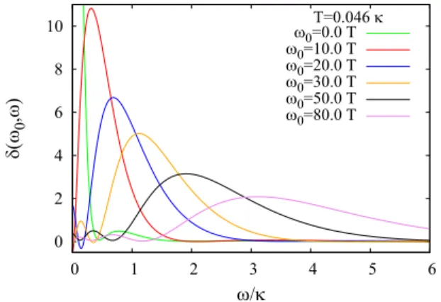
T=0.046 κ ω0=0.0 T ω0=10.0 T ω0=20.0 T ω0=30.0 T ω0=50.0 T ω0=80.0 T
FIG. 2. The resolution functionsδ(ω0,ω), obtained with standard Tikhonov regularization [see (41)] during the solution of the Green- Kubo relation for DOS (19). The parameterω0 labels the center of the resolution function. The value of the regularization parameter is λ=10−7. This setup will be used in all cases where we compute the DOS from the Monte Carlo data.
has a significant effect on the resulting spectral function. This setup will be used later for further calculations of the DOS.
To gain an accurate estimate of the statistical error in our spectral functions, we perform a data binning as follows.
Taking our original ensemble ofNconfHubbard field configu- rations generated according to the weight (15), we construct ˜N blocks ofNconf/N˜configurations. We are then left with several subsets of Euclidean time correlators,
{G(i)(τj),i=1, . . . ,Nconf}
→ {G(i)(τj),i=1, . . . ,Nconf/N˜}, . . . ,
{G(i)(τj),i=( ˜N−1)Nconf/N˜ +1, . . . ,Nconf}. (43) The number of blocks N˜ is chosen by examining the autocorrelation of the Euclidean correlator between different Hubbard field configurations and enforcing the condition Nconf/N˜ lmax, wherelmaxis the maximum autocorrelation length pertaining toG(τi), i=0,1, . . . ,Nτ−1. This condi- tion ensures that the size of each block is such that it contains numerous statistically independent configurations and each block is statistically independent of all the other blocks. Using these blocks of correlators, we construct ˜N spectral functions A¯iand calculate an average spectral function,
A¯avg≡ 1 N˜
N˜
i=1
A¯i, (44)
and its associated error σ( ¯A) for each frequency. We have found that this procedure yields a much better estimate of the statistical error than simply propagating the error in the Euclidean correlator to the spectral function through the relation in (32). Figure 1 demonstrates typical behavior of the statistical errors when we switch on the regularization.
If the regularization is not sufficient, the spectral function has huge statistical errors. Once we increaseλ, the errors are suppressed, and the spectral function converges to some stable average value. As mentioned previously (see Fig.3), the price for this smoothing is the enlargement of the width of all resolu- tion functions which may imply the loss of some information.
2 3 4 5 6 7 8 9 10
0.01 0.1 1 10 100 1000
half-peak width [T]
error of ρ (ω) at ω=0 Resolution function at ω=0
covariance matrix reg.
modified Tikhonov reg.
standard Tikhonov reg.
FIG. 3. The half-peak width of the resolution function centered around ω0=0 versus the statistical error. The calculation is per- formed with different regularization algorithms for the correlator G(τ) calculated on the lattice with spatial sizes Ns=20 and Nτ=160 for the interaction strengthU/κ=1.66, V /κ=0.62, and temperatureT /κ=0.046. The statistical error is controlled by the regularization parameterλ. The resolution functions are computed in the process of inverting the Green-Kubo relation for the DOS (19).
The width is given in units of temperature, and one can see that, as λvanishes, each curve converges to∼2. This is as expected as the resolution in frequency space ultimately is limited by the temperature.
We now compare all three types of regularization using the width of the resolution functions as a metric. The study is summarized in Fig.3where we plot the width at half maximum of the resolution function with the center atω0 =0 versus the statistical error of the reconstructed spectral function (again at ω0=0) for all regularization methods. The data for the DOS were used as a test case. As one can see, both types of Tikhonov regularization work better in the sense that they provide better resolution in the frequency domain while being equally efficient in suppressing statistical error. Or, in other words, for the Tikhonov regularization the statistical error is smaller for the same resolution in frequencies. One also can see that in practice the difference between the standard (41) and the modified Tikhonov (42) regularizations is negligible.
As a consequence, we will use the standard Tikhonov approach in all further calculations.
The algorithm for choosing the optimal value ofλis based on the “global relative error” for the spectral function,
G≡ 1 N0
ω0
σ[ ¯A(ω0)]
A¯avg(ω0), (45) where the sum in the above expression runs over the centers of the resolution functions andN0is the number of resolution functions with different centersω0. Our basic criterion for the choice ofλ is that the “global relative error” should be within the interval of 5–10%. We thus sufficiently suppress the statistical error while still maintaining good resolution in frequency space.
Using the quantity in (45) as a measure, we start from small λand increase it until we have obtained the desired statistical error. Typically, we have takenλ=10−7–10−5 in obtaining the results in this paper.
This primary regularization is enough to obtain reasonably good results for the DOS as one can see from Fig. 1.
-0.05 0 0.05 0.1 0.15 0.2 0.25
0 10 20 30 40 50 60 70 80
C(q, τ)
τ
initial correlator averaged correlator
(a)
-0.05 0 0.05 0.1 0.15 0.2 0.25
0 10 20 30 40 50 60 70 80
C(q, τ)
τ
initial correlator averaged correlator
(b)
FIG. 4. Two variants of correlator averaging. The charge-density- density correlatorC(q,τ) is calculated forU/κ=3.33, V /κ=1.26, andT /κ=0.046 using a lattice with spatial sizeNs=20 andNτ= 160 Euclidean time slices. The momentumqbelongs to theX-Mline in the Brillouin zone, which is the most physically interesting case (see below in Sec.V).
Unfortunately, for the case of the charge-density-density correlator, when we calculate the charge susceptibility by solving (26), this regularization is not enough. The source of the this problem is the very large autocorrelation between different points in Euclidean time for the correlatorC(q,τ). As a result, it exhibits long-range fluctuations which can be seen in Fig.4. We took the example correlatorC(q,τ) for the strongest interaction strength considered (U/κ=3.33, V /κ=1.26) with the momentum q directed along the X-M line in the Brillouin zone. This is the most physically interesting case and will be discussed in detail in Sec.V. After the application of the analytic continuation procedure, this oscillating correlator leads to a wildly fluctuating spectral function unless the regularization is so large that we hardly can resolve any structure due to very wide resolution functionsδ(ω0,ω).
The way in which we have modified the BG method to alleviate this problem is through the introduction of “interval averaging.” In this procedure, we take the correlator data {G(τi),G(τi); i=0,1, . . . ,Nτ−1}and map this to a new
Imχρ (ω, q)
ω/κ -0.1
0 0.1 0.2 0.3 0.4 0.5 0.6
0 2 4 6 8 10
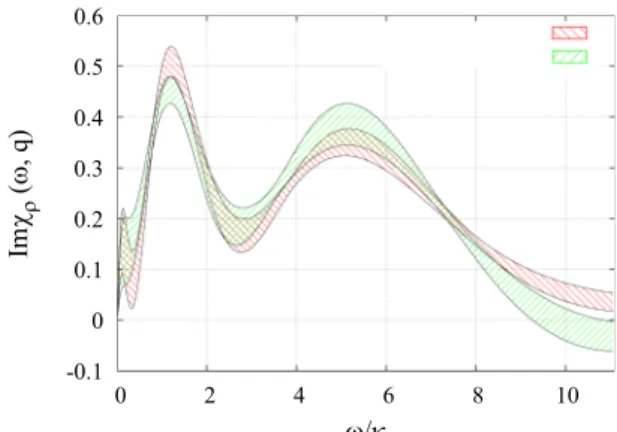
FIG. 5. Spectral functions Imχρ(ω,q) computed using the rela- tions (28) and (29) for two different variants of the averaged correlator shown in Fig.4. In both cases the ordinary Tikhonov regularization is used withλ=5.0×10⁻⁶. We plot the estimator for the spectral function obtained according to (30). The frequencyωcorresponds to the center of the resolution function, and the filled area shows the statistical error.
set{G( ˜˜ τj),G( ˜˜ τj); j =1, . . . ,Nint}where G( ˜˜ τj)≡ 1
N˜j
N˜j
i=1
G τi(j)
, (46)
Nτ =
Nint
j=1
N˜j, 1N˜j < Nτ. (47) After performing the procedure, we are left with a set of aver- aged values of the correlator calculated over certain intervals in Euclidean time. Due to the linearity of (19) and (26), one can construct {K( ˜˜ τj); j =1, . . . ,Nint} in an analogous manner and use these in the construction of the spectral function via the Tikhonov regularization. As a result, the spectral function will reproduce the averaged Euclidean correlator and will not follow the fluctuations within these intervals.
Typically, the signal-to-noise ratio of a Euclidean correlator G(τ) becomes worse as one approaches τ =β/2. Further- more, the correlations between adjacent points in Euclidean time are strong as one approaches this point. In light of this, we leave the points nearτ =0 untouched, whereas the points closer toβ/2 are bunched into intervals of longer length. In order to examine the dependence of the results on the choice of the intervals, we have performed the analytic continuation for the two different choices of intervals displayed in Fig.4.
The results of the analytic continuation are shown in Fig.5.
One can see that the two agree within the error bars, which indicates that the qualitative features of the spectral function do not drastically change for different variants of averaging.
In our calculations for the charge susceptibility we will use the first variant of averaging shown in Fig.4(a).
V. RESULTS
In this section, we present our results for the spectral functions. We perform all of our calculations with a spatial lattice size ofNs=20 andNτ =160 Euclidean time slices.
DOS (κ-1 )
ω/κ
(a)
U/κ=0.83, V/κ=0.5
0 0.1 0.2 0.3 0.4 0.5 0.6 0.7
0 1 2 3 4 5 6 7
DOS (κ-1 )
ω/κ
(c)
U/κ=3.33, V/κ=1.26
0 0.05 0.1 0.15 0.2 0.25 0.3 0.35 0.4 0.45
0 1 2 3 4 5 6 7
DOS (κ-1 )
ω/κ
(b)
U/κ=1.67, V/κ=0.63
0 0.1 0.2 0.3 0.4 0.5 0.6
0 1 2 3 4 5 6 7
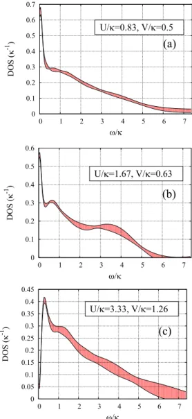
FIG. 6. Plot of the DOS for the lattice ensemble with electron-electron interaction (a)U/κ=0.83, V /κ =0.5, (b)U/κ= 1.66, V /κ=0.62, and (c)U/κ =3.33, V /κ=1.26. In all cases we have used a spatial lattice size of Ns =20 with Nτ=160 steps in Euclidean time and a temperature of T /κ=0.046. The standard Tikhonov regularization withλ=10−7is employed during the analytical continuation. Thus, in all cases, we have the same resolution in frequency. No additional averaging in Euclidean time is applied. The filled areas show the statistical error computed with the data binning procedure, and the frequencyωcorresponds to the center of the resolution function. The average value represents the estimator for the DOS computed according to (30). One can see the formation of the Hubbard bands, characterized by the peak at E/κ≈0.5, indicating that one is in the strongly coupled phase for the strongest interaction strength. For weaker interaction strengths we obtain a strong peak at zero energy indicating that the system is in the metallic phase.
Temperature is equal to T =0.046 in units of the hopping parameter κ. This temperature is lower then the one used in Ref. [13], but we really need it since the resolution of the BG method is limited by temperature. In order to justify our conclusions we also have performed one calculation for
two times higher temperatureT =0.092κ. For each strength of the electron-electron interaction we have generated∼103 Hubbard field configurations for the calculation of the relevant observables. Since the width of the resolution functions [quantityD in (33)] is bounded from below by temperature, the spacing between neighboring values of ω0 is equal to the temperature in our calculations. The upper bound forω0 is defined by the bandwidth where all considered spectral functions go to zero.
To make contact with the results of Ref. [13], we state the values of the parameters characterizing the interaction potential in our notation. The three sets of parameters used in Ref. [13] correspond to V ≈1.26 and U =4.4,8.2,10.4 (in units of the hopping parameterκ). In Ref. [13] the Mott transition was observed somewhere betweenU=8.2 andU = 10.4. Our first aim is to identify the real position of the phase transition from our nonperturbative Monte Carlo calculations.
For this purpose, we calculate the DOS for several pairs of UandV which characterize the electron-electron interaction.
The results from these calculations are presented in Fig.6.
One clearly can see that, even for the cases of U = 3.33, V =1.26 [see Fig. 6(c)], which is smaller than the smallest interaction strength from Ref. [13], the system is already in the insulating state. In this regime, the Hubbard bands have formed already, and the quasiparticle weight atω= 0 practically vanishes (due to finite temperature and the finite width of resolution functions, it cannot vanish completely).
In Fig.6(b), the DOS for the couplingsU=1.66, V =0.62 demonstrates that one is now firmly in the regime with well-defined quasiparticles atω=0. Finally, Fig.6(a)shows the DOS forU =0.83, V =0.5, which is deep in the metallic phase. These results show that the EDMFT analysis from Ref. [13] overestimates the critical couplingUc of the Mott transition for the Hubbard-Coulomb model. We emphasize
DOS (κ-1 )
ω/κ
U/κ=4.4, V/κ=1.26
0 0.05 0.1 0.15 0.2 0.25 0.3
0 1 2 3 4 5 6 7
FIG. 7. Plot of the DOS for the lattice ensemble with electron- electron interactionU/κ=4.4, V /κ=1.26, which corresponds to the weakest interaction strength studied in Ref. [13] (U∗=1.1 in their notation). We have used a spatial lattice size ofNs=20 with Nτ=160 steps in Euclidean time and two times higher temperature T /κ=0.092, which is almost equal to the one used in Ref. [13]. The setup for the analytic continuation is exactly the same as for Fig.6.
One can see that, in contrast to the results displayed in Ref. [13], the Hubbard bands are formed already, which suggests that the metal- insulator phase transition is shifted to a weaker interaction strength even at the same temperature.
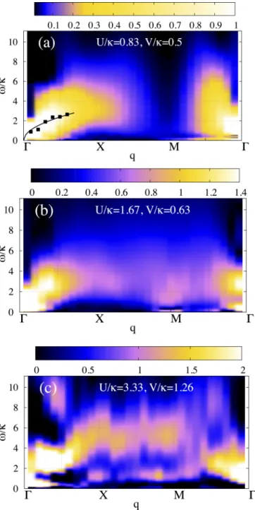
FIG. 8. Charge susceptibility for the square lattice Hubbard- Coulomb model for three different interaction strengths. The color scale corresponds to V(q)Imχρ(ω,q). For the spectral function Imχρ(ω,q) we use the estimated value after analytic continuation [see (30)]. The same lattice ensembles were used as in Fig.6. The standard Tikhonov regularization withλ=5×10⁻⁶and additional time averaging according to Fig.4(a)is used in all cases.
the fact that this is not a temperature effect as it is known that, for the square lattice Hubbard model, the phase transition is shifted to smallerU as the temperature decreases [8]. The results displayed in Fig.7show that, at twice the temperature of the ensembles in Fig.6, we are already in the insulating phase.
For these same values of the couplingU=4.4, V =1.26, and a slightly lower temperature, the authors of Ref. [13] find the system to be in the metallic phase.
V(q) Im χρ (ω, q)
ω/κ
X point
U/κ=0.83, V/κ=0.5 (x4) U/κ=1.67, V/κ=0.63 (x2) U/κ=3.33, V/κ=1.26 0
0.2 0.4 0.6 0.8 1 1.2 1.4 1.6
0 2 4 6 8 10
FIG. 9. Comparison of the spectral function for the charge-charge correlator at theXpoint for different interaction strengths. The lattice setup and the parameters of the analytic continuation procedure are identical to the ones used for Fig.8. The filled areas show the statistical error computed with the data binning procedure, and the frequency ωcorresponds to the center of the resolution function. The spectral functions for weaker interaction strengths are rescaled by factors of 2 and 4 in order to fit to the same scale.
Another difference is that one cannot confirm the situation reported in Ref. [13] for intermediate coupling: Near the phase transition the DOS had equally high peaks at zero energy and at some nonzero values of±E0. It is possible that something similar develops in Fig.6(b), but the second peak is too small and is basically within the error bars.
The results for the charge susceptibility in momentum space are presented in Figs.8and9 for the same lattice setup and interaction strengths as was presented for the DOS in Fig.6.
The plots start from the center of the Brillouin zone (point), continue out towards the edge of the BZ along thekxaxis, move along the edge of the BZ parallel to thekyaxis, and then finally return to the center of the BZ along the diagonal connecting the pointM≡(π,π) with. For the weakest interaction strength we have tried to reproduce the√q dispersion relation in the vicinity of thepoint [see Fig.8(a)]. The positions of the peaks at a given value of the momentum are depicted with black dots, and we have fitted their positions with the functionf(q)= C√
q. Despite the fact that the statistical fluctuations in the Monte Carlo data do not allow us to fully justify this fitting procedure, our data at least do not contradict the√qdispersion at weak interaction strength. When we move to largerUandV, the dispersion relation sufficiently changes, and at the strongest interaction strength, already in the insulating state, it finally splits into two branches. The splitting is most prominent along theX-M line in the Brillouin zone. The case of theXpoint is shown in Fig.9 separately for all three strengths of the electron-electron interaction. One clearly can see two peaks nearω=κandω=5κ.
VI. CONCLUSIONS
We have studied the Mott metal-insulator transition in the Hubbard-Coulomb model on the square lattice using unbiased quantum Monte Carlo calculations on finite clusters.
The hybrid Monte Carlo algorithm was used to effectively
study the system which contained a long-range interaction. In order to obtain the real-frequency spectral functions, we have developed a modified version of the Backus-Hilbert method for analytic continuation from Euclidean to real time. The metal-insulator phase transition was observed directly by the calculation of the density of states. The decrease in the DOS at zero energy and the formation of the Hubbard bands were observed across the phase transition. It was observed that the position of the phase transition is shifted sufficiently towards the weaker interaction strength in comparison to previous EDMFT predictions.
The behavior of the momentum-resolved charge suscepti- bility across the phase transition also was studied. These data were used to reveal the dispersion relation of the plasmons, both in the metallic and in the insulating phases. The main aim was to check the predictions from Ref. [13] concerning the splitting of the plasmonic dispersion relation into two bands in the region of the interaction strength close to the phase transition. The splitting indeed was observed in our Monte Carlo data. However, according to our calculations this phenomenon tends to emerge in the situation when the material is already in the insulating state.
The data presented in the paper can be used as a benchmark in the further development of methods for strongly correlated systems with long-range interactions.
The modified BG method developed in this paper also can be used in cases where a nonbiased estimate for the spectral function is important. The code used in the current paper is now accessible online [39].
ACKNOWLEDGMENTS
M.U. acknowledges inspiring and fruitful discussions with Prof. M. Katsnelson. The work of M.U. was supported by DFG Grant No. BU 2626/2-1. S.Z. acknowledges support by the National Science Foundation (USA) under Grant No. PHY-1516509 and by the Jefferson Science Associates, LLC under U.S. DOE Contract No. DE-AC05-06OR23177.
This work was supported partially by the HPC Center of Champagne-Ardenne ROMEO. C.W. acknowledges the warm hospitality of the staff of the University of Regensburg and would like to thank P. Buividovich for his financial support and for discussions in the early stages of the project. C.W. was sup- ported by the University of Kent, School of Physical Sciences.
[1]The Hubbard Model, edited by D. Baeriswyl, D. K. Campbell, J. M. P. Carmelo, F. Guinea, and E. Louis, Nato Science Series B (Springer, Berlin, 1995).
[2] P. A. Lee, N. Nagaosa, and X.-G. Wen,Rev. Mod. Phys.78,17 (2006).
[3] M. Imada, A. Fujimori, and Y. Tokura,Rev. Mod. Phys.70,1039 (1998).
[4] N. P. Armitage, P. Fournier, and R. L. Greene,Rev. Mod. Phys.
82,2421(2010).
[5] D. Rost, E. V. Gorelik, F. Assaad, and N. Blümer,Phys. Rev. B 86,155109(2012).
[6] J. Hubbard,Proc. R. Soc. London, Ser. A276,238(1963).
[7] J. Hubbard,Proc. R. Soc. Lonndon, Ser. A281,401(1964).
[8] T. Schäfer, F. Geles, D. Rost, G. Rohringer, E. Arrigoni, K.
Held, N. Blümer, M. Aichhorn, and A. Toschi,Phys. Rev. B91, 125109(2015).
[9] J. Lleweilun Smith and Q. Si,Phys. Rev. B61,5184(2000).
[10] R. Chitra and G. Kotliar,Phys. Rev. Lett.84,3678(2000).
[11] P. Sun and G. Kotliar,Phys. Rev. B66,085120(2002).
[12] F. Aryasetiawan and O. Gunnarsson,Rep. Prog. Phys.61,237 (1998).
[13] E. G. C. P. van Loon, H. Hafermann, A. I. Lichtenstein, A. N. Rubtsov, and M. I. Katsnelson,Phs. Rev. Lett.113,246407 (2014).
[14] S. Duane and J. B. Kogut, Phys. Rev. Lett. 55, 2774 (1985).
[15] M. V. Ulybyshev, P. V. Buividovich, M. I. Katsnelson, and M. I.
Polikarpov,Phy. Rev. Lett.111,056801(2013).
[16] P. V. Buividovich and M. V. Ulybyshev,Int. J. Mod. Phys. A31, 1643008(2016).
[17] P. V. Buividovich and M. I. Polikarpov,Phys. Rev. B86,245117 (2012).
[18] D. Smith and L. von Smekal, Phys. Rev. B 89, 195429 (2014).
[19] C. Winterowd, C. DeTar, and S. Zafeiropoulos, Magnetic Catal- ysis in Graphene, Proceedings, Meeting of the APS Division of
Particles and Fields (DPF 2015): Ann Arbor, MI, 2015 (APS, Ridge, NY, 2015).
[20] C. DeTar, C. Winterowd, and S. Zafeiropoulos,Phys. Rev. Lett.
117,266802(2016).
[21] C. DeTar, C. Winterowd, and S. Zafeiropoulos,Phys. Rev. B95, 165442(2017).
[22] G. Backus and F. Gilbert,Geophys. J. R. Astron. Soc.16,169 (1968).
[23] B. B. Brandt, A. Francis, H. B. Meyer, and D. Robaina,Phys.
Rev. D92,094510(2015).
[24] D. L. Boyda, V. V. Braguta, M. I. Katsnelson, and M. V.
Ulybyshev,Phys. Rev. B94,085421(2016).
[25] A. N. Tikhonov, Sov. Math.4, 1035 (1963).
[26] J. Hubbard,Phys. Rev. Lett.3,77(1959).
[27] R. L. Stratonovich, Soviet Phys. Dokl.2, 416 (1957).
[28] A. Mukherjee and M. Cristoforetti,Phys. Rev. B90, 035134 (2014).
[29] T. DeGrand and C. DeTar, Lattice Methods for Quantum Chromodynamics(World Scientific, Singapore, 2006).
[30] L. P. Kadanoff and P. C. Martin, Ann. Phys. (N.Y.) 24, 419 (1963).
[31] H. B. Meyer,Eur. Phys. J. A47,86(2011).
[32] S. J. Dong and K. F. Liu,Phys. Lett. B328,130(1994).
[33] G. S. Bali, S. Collins, and A. Schäfer,Comput. Phys. Commun.
181,1570(2010).
[34] A. S. Gambhir, A. Stathopoulos, and K. Orginos,SIAM J. Sci.
Comput.39,A532(2016).
[35] J. S. Przemieniecki,AIAA J.1,138(1963)
[36] Y. Nakahara, M. Asakawa, and T. Hatsuda,Phys. Rev. D60, 091503(1999).
[37] M. Asakawa, T. Hatsuda, and Y. Nakahara,Prog. Part. Nucl.
Phys.46,459(2001).
[38] G. Aarts, C. Allton, J. Foley, S. Hands, and S. Kim,Phys. Rev.
Lett.99,022002(2007).
[39] M. Ulybyshev and C. Winterowd, Green-kubo solver: Release 1.2 [https://doi.org/10.5281/zenodo.825606].