Measuring Counterparty Risk Development of innovative Methods in Light of Regulatory Reforms

Development of innovative Methods in Light of Regulatory Reforms

A dissertation in partial fulfillment of the requirements for the degree of Doktor der Wirtschaftswissenschaft (Dr. rer. pol.)

submitted to the

Faculty of Business, Economics, and Management Information Systems

University Regensburg

submitted by

Michael Kratochwil , M.Sc. in Finance

Advisors

Prof. Dr. Daniel R ¨ osch (University of Regensburg)

Prof. Dr. Harald Scheule (University of Technology Sydney)

Date of disputation: 29th of July 2020

First and foremost, I would like to thank Prof. Dr. Daniel R¨osch for his highly valuable input, continuous support and guidance. It was a pleasure and honour working with him on this research project. I want to express my gratitude to Prof. Dr. Harald Scheule for being my second advisor and a great host during my stay in Sydney.

I am grateful to all of my colleagues at the University of Regensburg and Dr. Nagler & Company GmbH for their support and more than anything, for an amazing time and long evenings. In particular, I wish to express my deepest gratitude to Dr. Martin Nagler for his support and for believing in me from the second we met. Furthermore, I would like to thank my co-author Dr.

Patrick B ¨uchel for his innovative ideas, challenging questions and many fruitful discussions.

Last but not least, I would like to thank my wonderful family and awesome friends. In particular, I would like to express my gratitude to my parents Inge and Kurt Kratochwil for doing an amazing job as parents.

I would like to dedicate this thesis to my wonderful wife Ramona. Thank you for your love,

your encouragement, and your patience over the last years. Thank you for believing in me, even

if I didn’t. It was quite a journey - but the best is yet to come.

Contents

List of Figures vi

List of Tables viii

Introduction 1

1 Credit Exposure under SA-CCR: Fixing the treatment of equity options 11

1.1 Introduction . . . . 12

1.2 Approaches for the determination of CCR exposures . . . . 14

1.2.1 Overview and regulatory developments . . . . 14

1.2.2 The new standardized approach (SA-CCR) . . . . 16

1.3 Regulatory status and discussions . . . . 20

1.4 Volatility analysis . . . . 23

1.4.1 Methods and data . . . . 23

1.4.2 Validation of SA-CCR parameters . . . . 24

1.4.3 Alignment with SA-TB risk-weights . . . . 26

1.5 Simulation study . . . . 29

1.5.1 Methods and data . . . . 29

1.5.2 Results for plain-vanilla options . . . . 31

1.5.3 Results for barrier options . . . . 32

1.6 Conclusion . . . . 34

1.A APPENDIX . . . . 36

1.A.1 Current Exposure Method (CEM) . . . . 36

1.A.2 SA-CCR Methodology . . . . 37

1.A.3 Transformation of SA-TB and SA-CCR risk-weights . . . . 42

1.A.4 Methodological foundations of the simulation study . . . . 45

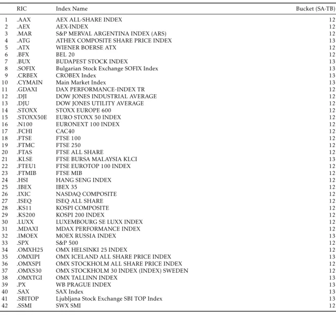
1.A.5 Selected indices for validation of SA-CCR parameters . . . . 47

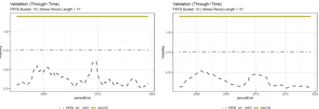
1.A.6 Through-time validation of SA-TB based volatilities . . . . 48

1.A.7 Results of the simulation study - Plain-vanilla options . . . . 53

1.A.8 Results of the simulation study - Barrier options . . . . 56

2 Computing valuation adjustments for CCR using a modified supervisory approach 59

2.1 Introduction . . . . 60

2.2 Methods for exposure quantification . . . . 61

2.3 Derivation of the modified SA-CCR . . . . 64

2.3.1 Replacement Costs . . . . 65

2.3.2 Potential Future Exposure . . . . 70

2.3.3 Multiplier . . . . 76

2.4 Calibration . . . . 78

2.4.1 Background and general considerations . . . . 78

2.4.2 Calibration of the modified SA-CCR . . . . 79

2.5 Empirical analysis . . . . 80

2.5.1 Methodology . . . . 80

2.5.2 Results . . . . 82

2.5.3 Implications for the supervisory SA-CCR . . . . 90

2.6 Conclusion . . . . 92

2.A APPENDIX | Analytical derivation of SA-CCR model foundations . . . . 94

2.A.1 Expected Exposure . . . . 94

2.A.2 Aggregating trade level add-ons . . . . 96

2.A.3 PFE multiplier formulation . . . . 97

2.A.4 Adjusted notional calculation by asset class . . . 101

2.B APPENDIX | Empirical analysis . . . 104

2.B.1 Calibration of the benchmark model (BMM) . . . 104

2.B.2 Input: Transactions and netting sets . . . 106

2.B.3 Output: IR profiles . . . 107

2.B.4 Output: FX profiles . . . 109

2.B.5 Output: Profiles for combined netting sets . . . 111

2.B.6 Output: Profiles for portfolios with perfect CSA . . . 112

2.B.7 Output: Profiles for portfolios with imperfect CSA . . . 112

2.B.8 Output: Profiles for FX options . . . 113

3 The KANBAN approach - A new way to compute forward Initial Margin 114 3.1 Introduction . . . 115

3.2 ISDA-SIMM™ . . . 116

3.2.1 Methodological overview . . . 116

3.2.2 Sensitivity requirements . . . 118

3.3 Forecasting initial margin requirements . . . 120

3.4 The KANBAN approach . . . 123

3.4.1 Modeling framework and general aspects . . . 123

3.4.2 Linear products . . . 126

3.4.3 Non-linear products . . . 130

3.5 Case study . . . 132

3.5.1 Methodology and data . . . 132

3.5.2 FX forward . . . 133

3.5.3 Interest rate swap . . . 135

3.5.4 Interest rate swaption . . . 137

3.5.5 IR swap portfolio . . . 139

3.6 Conclusion . . . 141

3.A APPENDIX | Background on modeling framework . . . 142

3.A.1 Cash flow concept . . . 142

3.A.2 American Monte Carlo (AMC) implementation . . . 145

3.B APPENDIX | Derivation of sensitivity calculations . . . 148

3.B.1 Delta sensitivities for linear products . . . 148

3.B.2 Vertex delta sensitivities for linear products . . . 151

3.B.3 Delta sensitivities for non-linear products . . . 155

3.B.4 Vega sensitivities for non-linear products . . . 156

3.C APPENDIX | Supplementary result data . . . 160

3.C.1 Interest rate swap . . . 160

3.C.2 Interest rate swaption . . . 161

3.C.3 Interest rate swap portfolio . . . 162

Conclusion 163

References 173

1.1 Equity single-name validation results . . . . 25

1.2 Equity index validation results . . . . 26

1.3 Through-time validation (bucket 5) . . . . 28

1.4 Through-time validation (bucket 12) . . . . 29

1.5 MSE results for European options (Single-Name (3Y), unmargined) . . . . 31

1.6 MSE results for European options (Index (1Y), unmargined) . . . . 32

1.7 MSE results for European barrier options (down-in call) . . . . 33

1.A.1 Through-time validation (bucket 1) . . . . 48

1.A.2 Through-time validation (bucket 2) . . . . 48

1.A.3 Through-time validation (bucket 3) . . . . 48

1.A.4 Through-time validation (bucket 4) . . . . 49

1.A.5 Through-time validation (bucket 5) . . . . 49

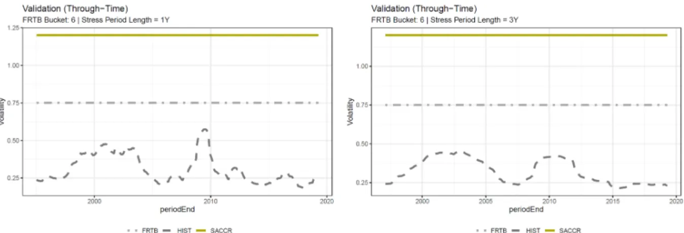
1.A.6 Through-time validation (bucket 6) . . . . 49

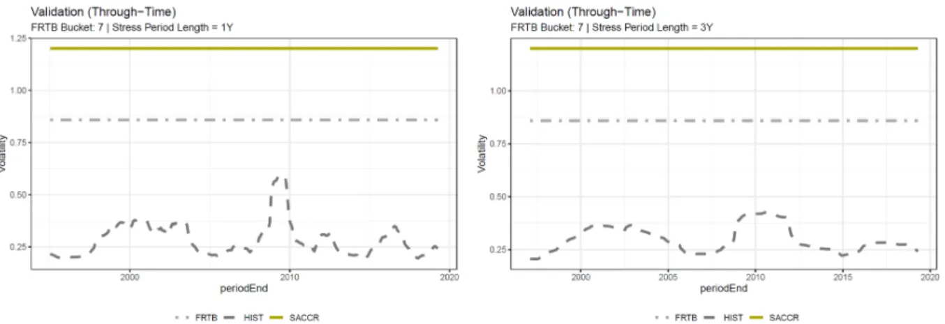
1.A.7 Through-time validation (bucket 7) . . . . 50

1.A.8 Through-time validation (bucket 8) . . . . 50

1.A.9 Through-time validation (bucket 9) . . . . 50

1.A.10 Through-time validation (bucket 10) . . . . 51

1.A.11 Through-time validation (bucket 12) . . . . 51

1.A.12 Through-time validation (bucket 13) . . . . 51

1.A.13 Through-time validation (SA-TB category: Size) . . . . 52

1.A.14 Through-time validation (SA-TB category: Economy) . . . . 52

1.A.15 MSE results for European options (Single-Name (3Y), unmargined) . . . . 53

1.A.16 MSE results for European options (Single-Name (3Y), margined) . . . . 53

1.A.17 MSE results for European options (Single-Name (1Y), unmargined) . . . . 53

1.A.18 MSE results for European options (Single-Name (1Y), margined) . . . . 54

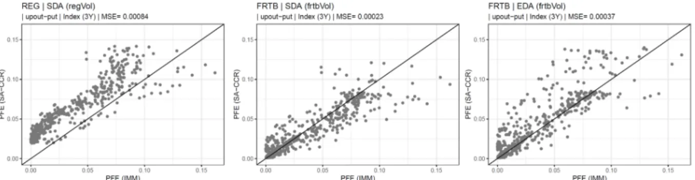
1.A.19 MSE results for European options (Index (3Y), unmargined). . . . 54

1.A.20 MSE results for European options (Index (3Y), margined) . . . . 54

1.A.21 MSE results for European options (Index (1Y), unmargined) . . . . 55

1.A.22 MSE results for European options (Index (1Y), margined) . . . . 55

1.A.23 MSE results for European barrier options (down-in call) . . . . 56

1.A.24 MSE results for European barrier options (down-in put) . . . . 56

1.A.25 MSE results for European barrier options (down-out call) . . . . 56

1.A.26 MSE results for European barrier options (down-out put) . . . . 57

1.A.27 MSE results for European barrier options (up-in call) . . . . 57

1.A.28 MSE results for European barrier options (up-in put) . . . . 57

1.A.29 MSE results for European barrier options (up-out call) . . . . 58

1.A.30 MSE results for European barrier options (up-out put) . . . . 58

2.1 Exposure profiles of an EUR 5Y ATM IR (payer) swap . . . . 82

2.2 Expected exposure of EUR 10Y IR payer swaps . . . . 83

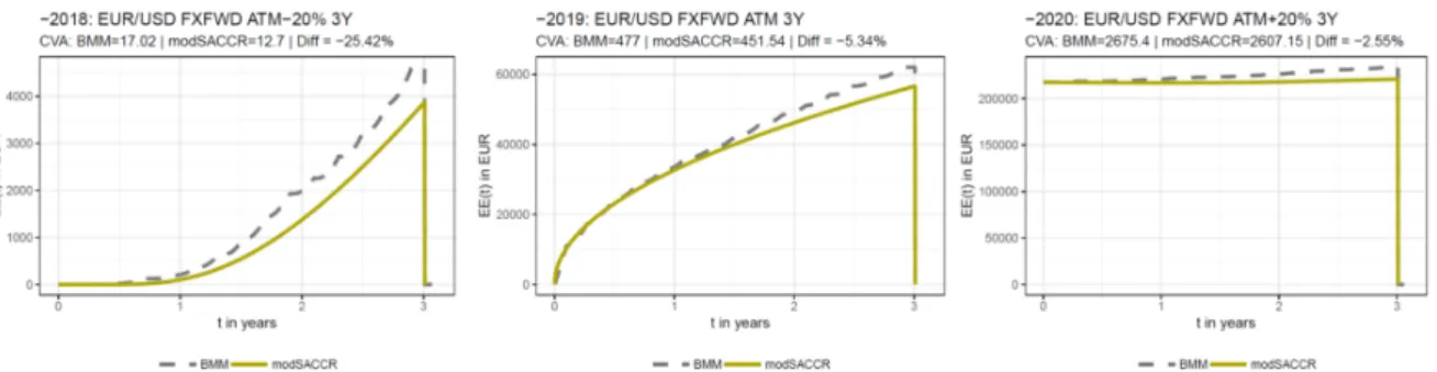
2.3 Expected exposure profile for FX forwards with different moneyness . . . . 85

2.B.1 Expected exposure of EUR 5Y IR payer swaps . . . 107

2.B.2 Expected exposure of EUR 5Y IR receiver swaps . . . 107

2.B.3 Expected exposure of EUR 10 IR payer swaps . . . 107

2.B.4 Expected exposure of EUR 7Y IR payer swaps . . . 108

2.B.5 Expected exposure of USD 5Y IR payer swaps . . . 108

2.B.6 Expected exposure of EUR/USD 1Y FX forwards . . . 109

2.B.7 Expected exposure of EUR/USD 3Y FX forwards . . . 109

2.B.8 Expected exposure of EUR/JPY 3Y FX forwards . . . 109

2.B.9 Expected exposure of EUR/GBP 3Y FX forwards . . . 110

2.B.10 Expected exposure of EUR/CHF 1Y FX forwards . . . 110

2.B.11 Expected exposure of USD/GBP 3Y FX forwards . . . 110

2.B.12 Expected exposure profile of IR multi-transaction netting sets . . . 111

2.B.13 Expected exposure profile of multi-transaction netting sets . . . 111

2.B.14 Expected exposure profile of IR multi-transaction netting sets . . . 111

2.B.15 Expected exposure profile of IR swaps with perfect CSA . . . 112

2.B.16 Expected exposure profile of FX forwards with perfect CSA . . . 112

2.B.17 Expected exposure profile of IR swaps with a CSA (TH=5.000,MTA=1.000) . . 112

2.B.18 Expected exposure profile of FX forwards with a CSA (TH=5.000,MTA=1.000) 113 2.B.19 Expected exposure profile of FX call options . . . 113

2.B.20 Expected exposure profile of FX put options . . . 113

3.1 Structure of ISDA-SIMM™ . . . 118

3.2 IM distribution at different viewpoints (FX forward) . . . 134

3.3 IM tenor profiles . . . 135

3.4 IM distribution at different viewpoints (IR swap) . . . 136

3.5 IM distribution at different viewpoints (IR swaption) . . . 139

3.6 IM distribution at different viewpoints (IR swap portfolio) . . . 140

3.7 Notional and IM tenor profile for IR swap portfolio . . . 140

3.B.1 Output from Monte Carlo pre-simulations . . . 158

List of Tables

1.1 Supervisory parameters for equity derivatives . . . . 20

1.2 Summary of validation results . . . . 24

1.3 SA-TB risk-weights: Transformation and validation . . . . 27

1.4 Definition of SA-CCR configurations . . . . 30

1.5 MSE results for plain-vanilla European options . . . . 32

1.6 MSE results for European barrier options . . . . 34

1.A.1 SA-TB risk-weights: Bucket definition and risk-weight transformation . . . . . 44

1.A.2 Selected indices for validation of SA-CCR parameters . . . . 47

2.1 CVA results for hypothetical IR swaps . . . . 84

2.2 CVA results for hypothetical FX forwards . . . . 86

2.3 CVA results for hypothetical combined netting sets . . . . 87

2.4 CVA results for collateralized portfolios (perfect CSA) . . . . 89

2.5 CVA results for collateralized portfolios (CSA: TH=5.000, MTA=1.000) . . . . 90

2.6 CVA results for FX options . . . . 91

2.B.1 Hypothetical netting sets for empirical analysis in section 2.5 . . . 106

3.1 ISDA-SIMM™ - Sensitivity inputs (examples) . . . 120

3.2 SIMM - Sensitivity inputs (FX forward) . . . 133

3.3 SIMM - Sensitivities over time (FX forward) . . . 134

3.4 IM distribution at di ff erent viewpoints (FX Forward) . . . 134

3.5 SIMM - Sensitivity inputs (IR swap) . . . 136

3.6 IM distribution at di ff erent viewpoints (IR swap) . . . 136

3.7 SIMM - Sensitivity inputs (IR swaption) . . . 137

3.8 IR vega sensitivity over time (IR swaption) . . . 138

3.9 IM distribution at different viewpoints (IR swaption) . . . 139

3.10 IM distribution at different viewpoints (IR swap portfolio) . . . 140

3.A.1 Trade object . . . 142

3.A.2 Example: IR floating cash flow . . . 143

3.A.3 Example: IR swap cash flows . . . 143

3.A.4 AMC variables . . . 145

3.B.1 Descriptive statistics of pre-simulation results . . . 158

3.C.1 LIBOR sensitivity over time (IR swap) . . . 160

3.C.2 OIS sensitivity over time (IR swap) . . . 160

3.C.3 EURIBOR sensitivity over time (IR swaption) . . . 161

3.C.4 OIS sensitivity over time (IR swaption) . . . 161

3.C.5 SIMM - Sensitivity inputs (IR swap portfolio) . . . 162

Motivation and area of research

A sound and stable financial sector is a critical and essential building block of modern economies.

Financial institutions act as intermediaries and support the alignment of money supply and lending as well as an efficient transfer of risks. The stability of the financial system is considered to be a crucial prerequisite for economic growth (BCBS (2011)). By pursuing their business activities, financial institutions take different types of risks. Some of these risk are taken deliberately, such as credit risk from lending transactions, others are inherited in the business activities themselves, such as operational or business risks. Financial institutions need to manage their risks properly to prevent losses and to ensure they are able to fulfill their contractual obligations at any time. Given the systemic importance of banking institutions and their stability, regulatory requirements are imposed to ensure the appropriate management of risks. For example, banks are required to hold a regulatory defined amount of capital to absorb potential losses from their business activities (BCBS (2011)). The quantification of capital requirements for different types of risk is a central aspect of supervisory oversight and an indispensable element of the regulatory framework. Financial institutions use various instruments to take, transfer and manage financial risks. In the past decades, derivative instruments have played a major role in the financial sector as they offer the possibility to synthetically take or close a risk position. Hence, derivatives can be used to efficiently transfer risks between counterparties.

When trading derivatives (bilaterally) over-the-counter (OTC), each counterparty has the risk of the other not meeting its contractual obligations (Gregory (2015)). Within the regulatory framework, this risk is referred to as Counterparty (Credit) Risk (CCR).

1

The terms

and

are used synonymously within this thesis.

The most challenging task in counterparty risk management is the modeling of credit exposures.

The measurement of credit exposures for derivatives and classical lending transactions di ff er in various aspects (Picoult (2004)). First, the future exposure of derivatives is uncertain, as it is a function of market parameters, while the exposure of lending risk transactions is usually known. Second, the risk in derivative transactions is bilateral, as a positive exposure can emerge for both counterparties in the future. Lending risk is generally unilateral, as the direction of the credit exposure is clearly defined by the underlying contract. Third, the mitigation of CCR often involves complex and dynamic risk mitigation techniques, such as margining, netting and clearing. The collateralization of lending risk transactions tends to be static and the methodological challenge lies in the valuation of collaterals. Finally, the quantification of CCR exposures is a laborious and complex task, while the exposure of lending risk transactions is deterministic in most cases. Given the bilateral nature of risk, the inherent uncertainty of future market parameters and the economic impact of dynamic risk mitigation techniques, the modeling of credit exposures from derivatives transactions requires advanced statistical concepts and in-depth quantitative knowledge (Picoult (2004)). The regulatory framework provides different approaches for the quantification of counterparty risk exposures. In general, institutions are able to choose between the application of an internal model method (IMM) or a regulatory standardized approach. While an IMM needs to adhere to a set of guidelines and requires supervisory approval, standardized approaches are less complicated, but result in a more conservative risk assessment (see BCBS (2006), BCBS (2014d)).

The Global Financial Crisis (GFC) from 2007-2009 revealed the significance of counterparty risk and the OTC derivatives market for the financial stability of the global economic system (FSB (2010)). During the crisis, financial institutions suffered tremendous losses in their derivatives business activities stemming from actual counterparty defaults as well as increasing Credit Valuation Adjustments (CVA). These losses jeopardized the survival of many financial institutions as well as the stability of the global financial system (Gregory (2010)). The Lehman Brothers bankruptcy in 2008 and the subsequent financial turmoil provided striking evidence for failures and shortcomings in the regulation of financial institutions and the OTC derivatives market. The G20 leader’s report of the 2009 Pittsburgh summit stated that “Major failures of regulation and supervision, plus reckless and irresponsible risk taking by banks and other financial institutions, created dangerous financial fragilities that contributed significantly to the current crisis.“

(G20 (2009)). As a response to the financial crisis, governments and supervisory authorities

developed additional regulatory requirements. Amongst other aspects, the G20 in 2009 agreed

to increase capital standards for banking institutions and to strengthen the regulation of the

OTC derivatives market (G20 (2009)). The corresponding policy measures included regulatory initiatives aiming at the reduction and mitigation of counterparty risk. There were two major areas of regulatory reform in this context. First, additional regulatory capital requirements were imposed to make banks more resilient against losses from counterparty risk. In this context, a variety of changes were made to the CCR capital framework (BCBS (2011)). Second, new rules for the trading of derivatives were imposed, such as mandatory central clearing for certain standard derivatives and the introduction of requirements for the collateralization of non-centrally cleared derivative transactions (FSB (2010)).

When looking retrospectively at supervisory activities in the past decade, it becomes clear that the Global Financial Crisis triggered a reform of the whole regulatory framework for banking institutions. At the time of writing, the process of regulatory conversion is not completed, as various regulatory changes are still to be finalized and implemented (BCBS (2017)). Nevertheless, the reform of the regulatory framework has already led to significant changes in the assessment of regulatory capital for counterparty risk. Under Basel II, the capital requirement for CCR was solely based on a default risk charge which is calculated in line with the capital requirements for credit risk based on a loan equivalent exposure measure (BCBS (2006)). An additional capital charge for CVA risk was introduced under Basel III to safeguard financial institutions against mark-to-market losses caused by the deterioration of the credit quality of counterparties.

Furthermore, additional requirements for the application of the IMM, such as the consideration of wrong-way-risk, were added to the framework, leading to higher capital requirements and more extensive qualitative model standards (BCBS (2011)). The existing standardized approaches for counterparty risk are considered outdated and not appropriate given the changed market conditions and standards as well as volatility levels observed during the GFC (BCBS (2013)). Hence, the BCBS published a new standardized approach for measuring counterparty credit risk exposures (SA-CCR) in 2014 (BCBS (2014d)). The SA-CCR will replace the existing standardized approaches going forward. This approach will be a central cornerstone of the future regulatory framework, as its results are used in subsequent regulatory measures, such as leverage ratio (BCBS (2014a)) and the CVA risk capital charge (BCBS (2019a)). Furthermore, under final Basel III rules (BCBS (2017)), the benefit from the application of internal methods will be bounded based on the result of the respective regulatory standardized approach.

Following the G20 declaration (G20 (2009)), additional rules and regulations for trading deriva-

tives were introduced. The aim of these new regulatory initiatives is the reduction of risk in the

financial industry and the protection of counterparties from the risk of another counterparty’s

default. The regulatory efforts are threefold. First, an obligation to clear certain standardized derivatives via central clearing counterparties (CCPs) is introduced. Second, additional report- ing requirements with respect to OTC derivatives trading activities are imposed to increase the transparency of the OTC market. Third, rules for the collateralization of non-centrally cleared derivatives are adopted to reduce the effect of counterparty defaults in OTC transactions. These rules include the mandatory exchange of variation margin (VM) and initial margin (IM) for certain bilateral transactions (FSB (2010), BCBS and IOSCO (2019)).

The emerging changes to the regulatory capital framework and the new rules for OTC derivatives trading will have a significant impact on the regulatory required capital for counterparty risk and the valuation of OTC derivatives. This leads to various theoretical and practical challenges for financial institutions when modeling counterparty credit risk exposures. This thesis aims to analyze and tackle three selected issues resulting from the introduction of the new standardized approach (SA-CCR) as well as the mandatory exchange of initial margin for non-centrally cleared OTC derivatives. The selected issues are handled in three independent research papers, which are presented in the chapters 1, 2 and 3 of this thesis. The following paragraphs provide a first introduction on the background, motivation and focus of each research paper.

Research paper I | Credit Exposure under SA-CCR: Fixing the treatment of equity options

The SA-CCR will replace the existing supervisory standardized approaches going forward. As

discussed above, its introduction will a ff ect a series of regulatory measures and most likely lead

to higher capital requirements (ABA et al. (2019)). The approach will be broadly applied and

has to be implemented by the majority of financial institutions, as its results will be utilized in

the determination of the capital output floor (BCBS (2017)). The banking industry generally

welcomes the introduction of the SA-CCR, as the approach o ff ers significant methodological

enhancements compared to its predecessors, such as the consideration of risk mitigating effects

from margining and over-collateralization. Nevertheless, there is ongoing discussion and

criticism regarding certain methodological aspects. Amongst others, the flawed treatment of

non-linear products as well as the overly conservative calibration of supervisory parameters,

in particular for equity products, have been bones of contention (ABA et al. (2019)). Given

the importance of the SA-CCR and its subsequent usage in the regulatory framework, a sound

understanding of its methodology, results and weaknesses is a crucial prerequisite for its

appropriate application by supervisory authorities and banking institutions. The first research

paper (see chapter 1) provides a theoretical and empirical analysis of methodological issues

regarding the treatment of equity options under SA-CCR. The research paper aims to increase

the understanding of the methodology and its weaknesses as well as to develop measures for improving the SA-CCR.

Research paper II | Computing valuation adjustments for CCR using a modified supervisory ap- proach

The calculation of CCR exposures is required for different aspects of risk management and valuation. First, credit exposures are required for the limitation of counterparty risk. Second, exposure results are used as inputs for the calculation of capital requirements. Third, expected exposure profiles are used in the calculation of various valuation adjustments, which are an integral part of derivatives pricing. The calculation of CCR exposures and especially time- dependent exposure profiles is a highly complex and laborious task. Small- and medium-sized financial institutions are, in most cases, not capable of maintaining an advanced CCR exposure model (EBA (2016)). Hence, there is undoubtedly a demand for more simple, but sufficiently accurate semi-analytical methods for exposure quantification. The SA-CCR involves significant enhancements compared to its predecessors. Amongst others, the new approach is able to recognize the risk mitigating effects from margining and provides a more sophisticated approach to netting and diversification (BCBS (2014d)). Furthermore, BCBS (2014b) provides a maximum of transparency on the methodological foundations of the approach. Hence, the SA-CCR offers a series of desirable features for the modeling of exposures while providing an accessible and holistic methodological framework. As discussed above, the SA-CCR has to be implemented by the majority of financial institutions. Hence, the utilization of the SA-CCR for the generation of time-dependent exposure profiles is an option worth considering, in particular for transactions not covered by advanced approaches. The second research paper (see chapter 2) develops a new semi-analytical approach based on the SA-CCR for determining time-dependent exposure profiles in the context of the CVA calculation.

Research paper III | The KANBAN Approach - A new way to compute forward Initial Margin

Given the emerging regulatory requirements regarding the collateralization of non-centrally

cleared derivatives, the majority of OTC transactions will be supported by the exchange of Initial

Margin (IM) in the future. ISDA provides a standard model (ISDA-SIMM™) for the calculation

of IM amounts, which essentially equals a sensitivity-based analytical VaR approach (ISDA

(2016), ISDA (2019)). This model is expected to become market standard for the calculation

of IM amounts for OTC derivatives. The bilateral exchange of IM significantly impacts capital

requirements, funding costs and the profitability of derivative transactions. Hence, IM amounts

must be considered when calculating CCR exposures. This requires the calculation of future IM requirements. The accurate forecasting of IM requirements is a di ffi cult and challenging task. In particular, the calculation of time- and path-dependent IM amounts in a Monte Carlo framework is complex and anything but straight-forward. In general, an approach for forecasting IM requirements should balance the computational burden and the accuracy of results. Most existing approaches are either inaccurate, hard to implement or not fully developed in order to be applied to complex practical situations. The third research paper (see chapter 3) introduces a new approach for forecasting IM requirements under ISDA-SIMM™.

In summary, this thesis aims to develop innovative solutions for prevailing and emerging issues in the area of CCR exposure modeling. The aforementioned challenges arise from changes in the regulatory framework as well as developments with respect to market standards in the OTC derivatives market. The thesis contributes to a wide field of scientific research on the modeling of counterparty credit risk exposures. The subsequent paragraphs provide an overview on existing literature focussing on methods for exposure quantification and forecasting of IM.

Literature

Over the past decades, the calculation of CCR exposures has been an active field of scientific research leading to a multitude of approaches and methods. According to Gregory (2015), there are three categories of approaches with different levels of sophistication: (1) advanced models, (2) semi-analytical and (3) parametric approaches. The most sophisticated way to model CCR exposures is the application of advanced approaches using Monte Carlo simulation. This involves complex tasks, such as the calibration of stochastic processes for the evolution of risk factors, the consideration of correlations and the modeling of collateralization. There is plenty of academic literature on various issues of the application of advanced exposure models (see, e.g., Picoult (2002), Canabarro and Duffie (2003) Pricso and Rosen (2005), Pykhtin and Zhu (2007)).

The literature on advanced methods covers di ff erent areas. For example, Picoult (2004) analyses the application of Monte Carlo (MC) simulation in the context of economic capital based on the results of Canabarro et al. (2003). The modeling of collateral and the impact of margining is also an important issue and has been analysed, amongst others, by Gibson (2005) and Pykhtin (2009). The emergence and ongoing improvement of advanced models also led to adoptions in the regulatory framework. Under Basel II (BCBS (2006)), banks are allowed to apply advanced exposure models for the purpose of measuring regulatory capital for counterparty risk for the first time.

2

Fleck and Schmidt (2005) provide a comprehensive analysis of the Basel II framework for counterparty credit risk.

While advanced methods deliver the most accurate results, their application requires a mag- nitude of personal and technical resources. Small- and medium-sized banks often lack the capabilities to develop and maintain advanced methods in the area of counterparty risk (Thomp- son and Dahinden (2013)). This results in a demand for less sophisticated approaches, which avoid the burdensome operation of a Monte Carlo simulation. This aspect has led to the devel- opment of various semi-analytical methods, which are based on certain assumptions regarding the evolution of risk factors and market values. Semi-analytical approaches have been designed for various asset classes and products (see, e.g., Brigo and Masetti (2005), Wilde (2005), Leung and Kwok (2005), de Pricso et al. (2007)). One early example is the approach of Sorensen and Bollier (1994). Their approach uses a strip of swaptions to model the exposure profile of an interest rate swap. In addition, the emergence of valuation adjustments for counterparty credit risk has led to various semi-analytical models for the approximation of product-specific CVA results (see, e.g., Kao (2016), Hull and White (2012), Cherubini (2013)). The second research paper (see chapter 2) aims to add an alternative and innovative method for measuring CCR exposures to the library of semi-analytical approaches.

Parametric approaches measure CCR exposures based on a few simple parameters. According to Gregory (2015), most parametric approaches model CCR exposure via a combination of the current exposure and an add-on for the potential future exposure. There is scarce academic literature regarding parametric approaches, but the concept is often utilized by regulators as the basis for regulatory standardized approaches. Under Basel II (BCBS (2006)), banks not applying an IMM are able to choose between two standardized approaches: Current Exposure Method (CEM)

and Standard Method (SM). Both approaches are parametric approaches, where the calculation of exposure is based on supervisory prescribed risk-weights.

The new standardized approach SA-CCR features elements of semi-analytical and parametric approaches. BCBS (2014b) and BCBS (2014d) provide comprehensive information on the SA-CCR methodology and its model foundations. The introduction of the SA-CCR led to a variety of literature regarding the evaluation of the new approach (see, e.g., Albuquerque et al. (2017), ABA et al.

(2019), Berrahoui et al. (2019)). The first research paper (see chapter 1) amends this research by dealing with weaknesses of the SA-CCR regarding the treatment of (non-linear) equity products.

The increasing importance of Initial Margin (IM) in the OTC derivatives market results in the requirement of forecasting IM amounts to model the e ff ect from the exchange of IM on CCR exposures. Various approaches for forecasting IM requirements are discussed in recent

3

Please note that the CEM has already been introduced in the Basel I framework (BCBS (1988), BCBS (1995)).

4

A comprehensive discussion of the Basel II standardized appraoches is provided by Fleck and Schmidt (2005).

academic research. A series of research papers propose the calculation of forward IM based on dynamic initial margin models (see Andersen et al. (2017a), Andersen et al. (2017b), Anfuso et al. (2017), McWalter et al. (2018)). These dynamic margin models are based on regression techniques, utilizing existing scenario information from the Monte Carlo simulation. Chan et al. (2017) provide an overview and evaluation of different regression approaches. Under ISDA-SIMM™ the task of forecasting IM reduces to the calculation of forward sensitivities, as these are the only dynamic time-dependent model inputs. There are various concepts for the calculation of forward sensitivities which can be applied to forecast IM amounts. Fries (2019), Fries et al. (2018) and Antonov et al. (2017)) use the concept of Adjoint Algorithmic Di ff erentiation (AAD) based on the work of Giles and Glasserman (2006) and Capriotti (2011).

Zeron and Ruiz (2018) utilize the concept of Chebyshev Spectral Decomposition to compute the required forward sensitivities. The third research paper (see chapter 3) broadens this area of research by introducing an innovative approach for forecasting IM requirements in an existing Monte Carlo framework.

Contributions

This thesis contributes to the literature on modeling counterparty credit risk exposures and adds innovative methods to the counterparty risk management toolbox. The main contributions of this thesis can be structured according to the independent research papers. These research papers are presented within the chapters 1, 2 and 3 of this thesis.

Contribution I | Credit Exposure under SA-CCR: Fixing the treatment of equity options

The first research paper (see chapter 1) develops and explores potential measures to improve the treatment of equity options under the SA-CCR. Based on a methodological deep-dive on the SA-CCR’s model foundations, an empirical analysis is conducted, in which the supervisory parameters are validated and the resulting exposures are benchmarked against an advanced model. The results of the analysis reveal the overly conservative calibration of supervisory parameters for equity transactions as well as the weaknesses of the SA-CCR in coping with non-linear products. Furthermore, it is found that the supervisory calibration for equity transaction clearly lacks granularity, leading to insufficient risk sensitivity of results. Given these findings, measures for improving the SA-CCR methodology are proposed. This includes the alignment of the calibration with the standardized approach for market risk (SA-TB) as well as the utilization of economic delta adjustments for the treatment of non-linear products.

The application of economic instead of supervisory delta adjustments offers improvement, but

should be accompanied by regulatory guidelines to ensure a consistent implementation across institutions. The alignment of the standardized approaches for CCR and market risk is proven to be beneficial for the risk sensitivity of the SA-CCR and would significantly contribute to the consistency of the regulatory capital framework for derivative products. In summary, the first research paper fosters the sound understanding of the SA-CCR’s methodological framework and associated weaknesses regarding the treatment of (non-linear) equity products. It provides measures for improvement of the SA-CCR methodology. In particular, the idea of aligning regulatory standardized approaches for market and counterparty risk is explored by theoretical and empirical analysis based on comprehensive historical data.

Contribution II | Computing valuation adjustments for CCR using a modified supervisory approach The second research paper (see chapter 2) introduces a fast and simple semi-analytical method for the calculation of time-dependent exposure profiles in the context of CVA quantification.

This new approach is a modified version of the supervisory SA-CCR. For an appropriate applica- tion, various adjustments are conducted on the supervisory framework. Within the research paper, these adjustments are derived and a risk-neutral calibration of the modified SA-CCR is established to ensure consistency with requirements defined by the accounting framework (IFRS 13). The modified SA-CCR offers a holistic framework covering a variety of asset classes and financial instruments. In a benchmark study, the modified SA-CCR is used to calculate exposure profiles and CVA results for a set of hypothetical netting sets involving commonly used derivative products, such as interest rate swaps and FX forwards. The results are com- pared to the outcome of an advanced benchmark model. The findings clearly indicate that the modified SA-CCR captures time-dependent and product-specific exposure dynamics and produces su ffi ciently accurate CVA results for accounting purposes. The modified SA-CCR provides an alternative and innovative semi-analytical modeling framework with significant enhancements to current industry practices regarding the calculation of CVA for transactions not covered by advanced models. As the new approach is a modification of the supervisory SA-CCR, institutions are able to leverage on existing or future implementations of the SA-CCR.

Hence, the approach is of high practical relevance for all kinds of financial institutions involved in derivative trading activities.

Contribution III | The KANBAN Approach - A new way to compute forward Initial Margin

The third research paper (see chapter 3), presents an innovative approach for forecasting

IM requirements under ISDA-SIMM™ based on forward sensitivities. This approach offers a

framework for the calculation of time- and path-dependent sensitivities in a Monte Carlo based exposure model. The KANBAN approach utilizes existing elements of the exposure model, such as cash flow objects and the pricing of non-linear instruments via American Monte Carlo (AMC).

The technical design of the approach is based on principles adopted from industrial just-in- time manufacturing. Cash flows are used as central objects, as they carry the comprehensive information for the production of forward sensitivities which can be interpreted by a central market data service. This enables a lean ”on-the-fly” generation of path- and time-dependent sensitivities. The KANBAN approach o ff ers a series of advantages over existing methods for the calculation of forward Initial Margin. First, the approach is much faster compared to classical

“bump-and-run“ approaches, as each cash flow is processed independently and sensitivities are calculated simultaneously instead of successively. Second, the KANBAN approach uses only information and methodological building blocks which are already implemented in the prevailing model framework. Hence, no additional model risk is added to the counterparty risk and valuation framework. Third, the new approach is applicable to any financial instrument, as the calculation of sensitivities is based on the unified representation of financial instruments as a series of cash flows. The research paper includes the methodological foundation of the KANBAN approach and a case study, in which the methodology is applied to standard financial products and an interest rate swap portfolio.

Structure

The thesis is structured alongside the three independent research papers with varying co- authors.

Chapter 1 presents the first research paper on the calculation of credit exposure under the new supervisory standardized approach (SA-CCR) and particularly the associated treatment of equity options. In chapter 2, a modified SA-CCR approach for the calculation of valuation adjustments for counterparty credit risk is introduced and discussed. Chapter 3 is dedicated to the development and application of a new methodology for forecasting initial margin amounts.

The Conclusion summarizes the thesis by discussing main results and providing an outlook for future research in the area of counterparty credit risk.

5

At the beginning of each chapter, information with respect to the current status of the paper and the respective co-

author(s) is provided. As the studies have been submitted to different journals with varying formal requirements,

there are minor formal differences across the chapters of this thesis.

Credit Exposure under SA-CCR:

Fixing the treatment of equity options

This chapter corresponds to a working paper with the same name (submitted to Journal of Credit Risk, currently under review).

Abstract

The new standardized approach for measuring counterparty credit risk exposures (SA-CCR) will replace the existing regulatory standard methods for exposure quantification. There is ongoing discussion with respect to the calibration and appropriate treatment of non-linear products under the SA-CCR. Especially, the calibration of supervisory parameters for equity derivatives has been a bone of contention. Furthermore, the SA-CCR struggles with the adequate reflection of non-standard options. Our paper provides empirical evidence that the SA-CCR parameters are not aligned with historically observed volatilities. We explore a potential alignment of the SA-CCR with the new standardized approach for market risk (SA-TB) as well as the application of economic delta adjustments for path-dependent equity products. Our results demonstrate that an alignment of SA-CCR and SA-TB could lead to a significantly improved risk assessment for equity derivatives.

Keywords: Counterparty Credit Risk; SA-CCR; Regulatory Capital; Credit Exposure

JEL classification: G01, G21, G32

1.1 Introduction

Counterparty Credit Risk (CCR) has been a main source of loss during the Great Financial Crisis (GFC). Furthermore, CCR significantly contributes to banks’ overall risk-weighted Assets (RWA). Hence, the assessment of minimum capital requirements for CCR has been a focus of regulators in the past decade. Especially the appropriate measurement of the Exposure at Default (EAD) for derivatives has been subject to ongoing discussions, as the existing approaches are considered to be outdated. The existing standardized approaches are used broadly in the banking industry. In general, even banks with an approved internal model (IMM) for CCR do not have approval to use the IMM for all products and / or subsidiaries (Thompson and Dahinden (2013)). The Basel Committee on Banking Supervision (BCBS) decided to review the standardized methods for measurement of CCR exposures and developed a new approach for exposure quantification (SA-CCR) (BCBS (2014d)).

The EAD calculated under the SA-CCR serves as input for the calculation of other regulatory measures, such as leverage ratio, large exposure framework, CVA risk capital charge and the CCP hypothetical capital calculation (BCBS (2017)). Hence, all banks must implement the SA-CCR irrespectively of the application of an internal model. Furthermore, there is ongoing discussion to use the results produced by regulatory standardized approaches as basis for the limitation of the capital benefits from the application of internal models (BCBS (2017)). Given the broad usage of the SA-CCR and its subsequent impact on various regulatory measures, we believe that the SA-CCR is a major cornerstone of the future regulatory framework. Thereby, systemic misjudgement of risk by the SA-CCR will not only affect capital requirements for CCR, but the regulatory framework as a whole.

The industry generally supports the replacement of the existing standardized approaches by the SA-CCR (OCC et al. (2019)).

Nevertheless, there are enduring concerns regarding a significant increase of capital requirements due to the conservative calibration and lack of risk sensitivity of the SA-CCR. There is ongoing discussion with respect to various flaws and shortcomings of the SA-CCR in Europe and the US. One area of concern is the conservatism of the calibration.

According to ABA et al. (2019) a recalibration of the supervisory factors and volatilities for equity products would reduce the burden for financial institutions. As stated by OCC et al.

(2019), various stakeholders suggested to align the SA-CCR parameters with risk-weights of

1

This was made clear by leading industry associations throughout the consultation process, which started with the

publication of the consultation paper in 2013 (BCBS (2013)).

the new standardized approach for market risk (SA-TB) (BCBS (2019b)). This would lead to a consistent assessment of risk and an increase of the risk sensitivity of the SA-CCR. In addition, potential drawbacks from using a supervisory delta adjustment formula based on Black &

Scholes for exotic options were addressed multiple times by various industry bodies. They suggest allowing banks to use their own proprietary delta values to avoid a disconnect between the calculation of capital requirements and actual risk management.

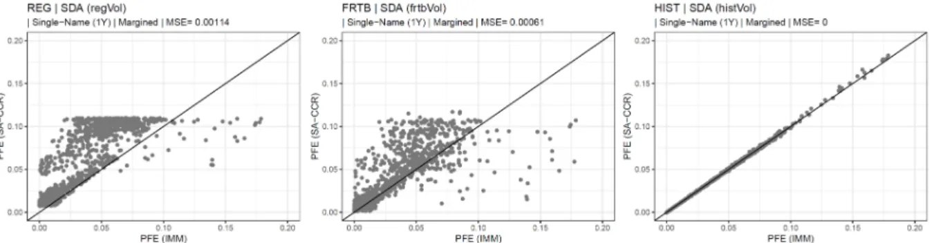
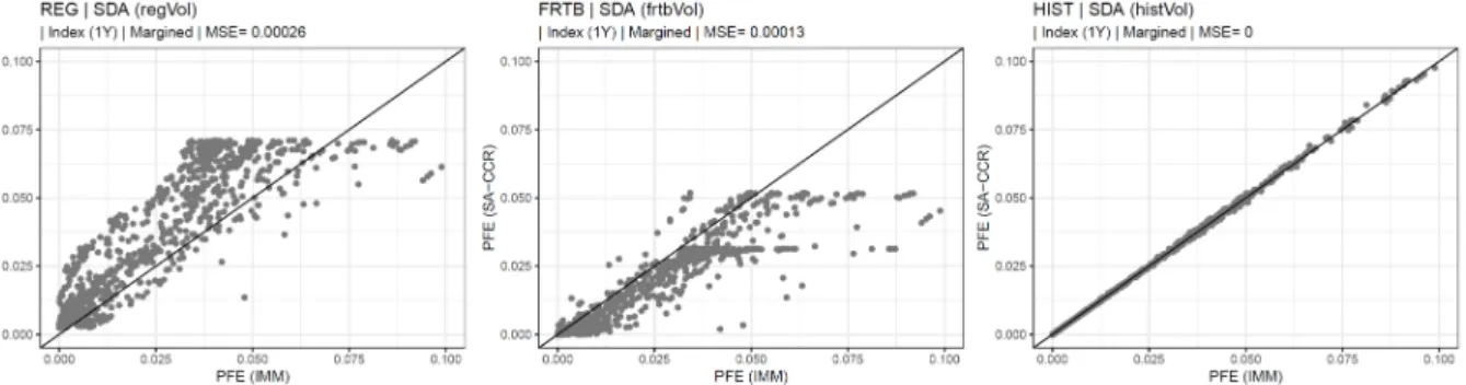
Our paper provides the following contributions. First, we provide a theoretical contemplation of the calibration and treatment of equity options under the SA-CCR. Second, we conduct an empirical analysis to validate the supervisory parameters and to benchmark the results from the SA-CCR against an advanced model. Based on the outcome of this analysis, we identify flaws of the SA-CCR and suggest improvements to the regulatory methodology for measuring CCR exposures. Our paper focuses on the calibration and treatment of equity options under the SA-CCR. Equity derivatives have smaller trading volumes compared to interest rate and foreign exchange derivatives (BCBS (2018b)). Nevertheless, the quantification of their exposure is often subject to standardized approaches, as only 70% of banks with IMM approval use their internal model for plain-vanilla and exotic equity derivatives (Thompson and Dahinden (2013)).

Hence, the handling of equity derivatives is considered an important and challenging field of application for standardized approaches.

We find that the calibration of the SA-CCR is overly conservative for most equity underlyings.

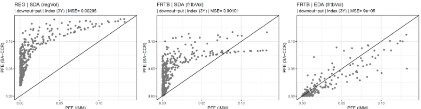
Furthermore, there is a lack of granularity in calibration, limiting the ability of the approach to properly reflect the risk of most underlyings. These issues lead to a significant over-estimation of risk for equity derivatives. Introducing a more granular and risk sensitive calibration approach would improve the results of the SA-CCR while keeping a reasonable level of complexity. Our results indicate that an alignment of the SA-CCR with the new standardized approach for market risk (SA-TB) would significantly enhance its risk sensitivity. In addition, the usage of economic approaches for the calculation of the delta adjustment parameter would also increase the risk sensitivity of the SA-CCR with respect to barrier options. Nevertheless, the application of economic delta adjustments needs to come along with additional regulatory guidelines to ensure a consistent implementation and results across institutions.

The remainder of this paper is structured as follows. Section 1.2 provides a short overview

of existing regulatory approaches for the measurement of CCR exposures and introduces the

SA-CCR, including its methodological foundations. A thorough understanding of the SA-CCR

methodology is a prerequisite for the subsequent discussion and empirical analysis. Readers

acquainted with the regulatory capital framework for CCR and the methodological foundations of the SA-CCR might decide to skip this section. We elaborate on the current regulatory status and ongoing methodological discussions in Section 1.3. The empirical part of this paper is structured as follows. First, we perform a volatility analysis (section 1.4) based on historical data to assess the need for recalibration of the supervisory parameters and the appropriateness of SA- TB risk-weights. Second, we conduct a simulation study (section 1.5) to assess the performance of

different SA-CCR calibrations and configurations based on hypothetical European plain-vanilla and barrier options. Section 1.6 summarizes the main conclusions and recommendations.

1.2 Approaches for the determination of CCR exposures

1.2.1 Overview and regulatory developments

In order to determine the default risk capital requirements for derivatives, banks must calculate the EAD for those transactions. The calculation of exposure values is performed for a set of positions within a legally enforceable netting agreement. The resulting EAD values serve as input for the calculation of regulatory capital requirements for default risk. The calculation of exposure values for CCR is considered a time-consuming and expensive task, as running the necessary simulations requires a high amount of computational power. Hence, there is a multitude of academic research on the optimization of calculation processes and simplification of methodology via the development of semi-analytical approaches. For example, Ghamami and Zhang (2014) provide an efficient Monte Carlo framework to decrease the computational time needed for the estimation of regulatory exposure measures. Orlando and H¨artel (2014) develop a parametric approach that estimates the exposure as the sum of current and potential future exposure, while Pykhtin and Rosen (2010) introduce a semi-analytical approach which is capable of reflecting the impact of collateralization on CCR exposures.

Under the current regulatory framework, there are different approaches for calculating the EAD

for derivative transactions (BCBS (2011)). On the one hand, there are regulatory standardized

approaches, while on the other hand institutions may apply internal models. Since the intro-

duction of Basel II (BCBS (2005)), banks are allowed to use their own internal exposure models

to estimate the credit exposure of derivative transactions within the regulatory capital frame-

work (Internal Model Method(IMM)). The internal model needs to adhere to quantitative and

qualitative requirements. The application is subject to supervisory approval. When applying

an Internal Model Method (IMM), the EAD for each netting set is defined as the product of a scaling factor (α) and the E ff ective Expected Positive Exposure (EEP E).

Under Basel III (BCBS (2011)), the EEP E is defined as the maximum of an EEP E calculated under stressed and current market data.

The regulatory framework currently offers a set of standardized approaches for exposure quantification. The Current Exposure Method (CEM) as well as the Standardized Method (SM) are simple and parametric approaches providing an approximation of the EAD. While the CEM is used by the majority of financial institutions, the SM is hardly applied within the financial industry (EBA (2016)).

CEM provides an approximation of the EAD as the sum of the current exposure (replacement costs) and an add-on for potential future exposure (PFE).

CEM has been criticized for various reasons in the past and is considered outdated. The BCBS summarizes the critique towards CEM in the following three main issues (BCBS (2013)). First, there is no differentiation between netting sets with and without margin agreements. Hence, the risk mitigation effects from margining are not rewarded within the regulatory capital framework. Second, the calibration of the supervisory parameters is outdated and does not consider volatility levels observed during the GFC. Third, the CEM involves a very simplistic recognition of diversification, when aggregating trade-level add-ons. In general, there has been ongoing criticism by members of the industry as well as academics.

An additional issue is the lack of risk sensitivity. Transactions of the same asset class and the same maturity will always have the same PFE under the CEM, regardless of their further, probably different, features (Gregory (2010)). Especially for options and other non-linear positions the lack of consideration of these features leads to unreasonable results.

Driven by this criticism, the BCBS has developed a new standardized approach (SA-CCR) to overcome the shortcomings of existing approaches and to align the regulatory treatment of derivatives with current market practices (BCBS (2013)). Going forward, the option to use an IMM model will persist, while the CEM and the SM will be replaced by the SA-CCR. The SA-CCR is more complex compared to CEM and aims to provide a reasonable risk sensitive exposure measure considering risk mitigation techniques as well as the moneyness of the netting set and the subsequent positions. Furthermore, the calculation procedure for the PFE takes

2

The correction-factor (α) is set to 1.4 and is introduced to account for systemic model errors as well as the missing consideration of general wrong-way risk in the regulatory CCR framework. For further information on the interpretation and role of the

3

According to EBA (2016) there are only two banks in Europe applying the SM.

4

A more detailed outline of the CEM is provided in APPENDIX 1.A.1.

5

Please refer to Fleck and Schmidt (2005) and Pykhtin (2014) for a comprehensive discussion of critique towards

CEM.

into account the non-linearity of products. The new approach can capture risk mitigation through margining, as there is a distinction between margined and unmargined netting sets. For margined netting sets, a shorter risk horizon is applied compared to unmargined netting sets (1 year), when calculating the PFE. Additionally, the SA-CCR allows for hedging and netting within the main asset classes via the introduction of hedging sets and subsets. Another key improvement compared to CEM is the enhanced reflection of over-collateralization.

1.2.2 The new standardized approach (SA-CCR)

General structure and interpretation

According to BCBS (2014b), the SA-CCR shall provide an approximation of the EAD under IMM, which is defined as the product of the α-factor and the Effective Expected Positive Exposure (EEPE). The SA-CCR defines the netting set EEPE as the sum of replacement costs (RC) and potential future exposure (P FE). Therefore, the fundamental structure of the SA-CCR is very close to the CEM but follows the basic idea of the IMM:

EAD

= α · EEP E

= α · (RC + P FE) ≈ EAD

(1.1) The SA-CCR is calibrated to stressed (historic) market data in order to achieve a conservative approximation. Furthermore, the α-factor is transferred from the IMM formulation. While the structure of the approach is very similar to CEM, the calculation of RC and P FE have been revised. For the calculation of RC the main improvement to CEM is the consideration of margining. In contrast, the calculation of the P FE component has been completely revised and a new methodological framework was introduced. Hence, we focus on the presentation and discussion of the P FE calculation in the subsequent paragraphs.

The P FE aims to quantify the risk of an increase in exposure due to a change in the market value of the netting set during a predefined risk horizon. Under the SA-CCR, the P FE term is defined as the product of the aggregated add-on on netting set level and a multiplier. The multiplier is a function of the netting set’s market value, volatility-adjusted collateral value and the aggregated add-on. In summary, the multiplier can be interpreted as a scaling factor for the PFE add-on with respect to the moneyness of the netting set.

6

APPENDIX 1.A.2 provides an overview of the calculation of

under the SA-CCR.

7

Detailed information and the derivation of the multiplier formula are available in BCBS (2014b) and BCBS

(2014d).

PFE add-on calculation

BCBS (2014b) offers a detailed description of the methodological framework for add-on calcu- lation.

The add-on calculation is performed based on the assumption of zero market values (V

(t

) = 0) and the absence of collateral (C

(t

) = 0). Furthermore, it is assumed that there are no cash flows within the risk-horizon of 1 year. The market value of transactions is assumed to follow an arithmetic Brownian motion with zero drift and constant volatility. Under these assumptions, we obtain the following analytical solution for the expected exposure (EE) of a netting set (k) at time t:

EE

(t) = σ

(t) · φ(0) ·

√

t (1.2)

where σ

(t) equals the annualized volatility of the netting set’s market value at t and φ(0) is defined as the standard normal probability density: φ(0) = 1/

√

2π. This formulation is the basis for the calculation of add-ons for margined and unmargined netting sets. The add-on for unmargined netting sets represents a conservative analytical approximation of the EEP E for a risk horizon of one year. We are able to derive an analytical solution using an EE profile based on equation (1.2) and applying a floor of 1 year to all trade maturities:

AddOn

= EEP E

= 2

3 · φ(0) · σ

(0) · p

1year (1.3)

This equation can be restated at trade-level.

Flooring all trade maturities at 1 year would produce unreasonable results and lead to an over-estimation of hedge e ff ectiveness for short- dated trades. Hence, a maturity factor(MF

) is introduced at trade-level to account for maturities (M

) smaller than 1 year:

AddOn

= 2

3 · φ(0) · σ

(0) · p

1year · MF

(1.4)

where MF

for transactions in an unmargined netting set is defined as:

MF

= s

min(M

, 10d)

1year (1.5)

The add-on for margined netting sets is defined as the potential increase in exposure over the Margin Period of Risk (MPOR). Based on the assumptions of zero market value and absence of

8

The following methodological discussion is based on BCBS (2014b).

9

For a detailed mathematical representation, please refer to APPENDIX 1.A.2.

10

For the detailed mathematical derivation, please refer to APPENDIX 1.A.2.

11

For the respective mathematical proof, please refer to APPENDIX 1.A.2.

collateral, this amount is defined based on equation (1.2):

AddOn

= EE

(MP OR) = φ(0) · σ

(0) ·

√

MP OR (1.6)

In accordance with the add-on calculation for unmargined netting sets, we can restate this equation at trade-level. In order to arrive at a consistent formulation for the trade-level add-on, we formulate the add-on for margined netting sets in line with equation (1.4) and introduce a maturity factor for margined netting sets (BCBS (2014b)):

MF

= 3 2 ·

s

MP OR

1year (1.7)

Hence, the only difference between the add-on calculation for margined and unmargined nettings sets is the definition of the maturity factor. For the calculation of the SA-CCR PFE add-on, each transaction is allocated to one of five risk categories (EQ, IR, CR, CO, FX) based on its primary risk factor.

To keep the calculation fast and simple, the SA-CCR does not use trade-level volatilities but a simple set of parameters. According to BCBS (2014d), the add-on at trade-level is defined as the product of a supervisory factor (SF

), an adjusted notional amount (d

), the supervisory delta adjustment (δ

) and the maturity factor (MF

)

:

AddOn

= SF

· d

· δ

· MF

(1.8) We obtain the following definition of the trade-level market value volatility (σ

) at t = 0 by inserting equation (1.4) into equation (1.8) and solving for σ

:

σ

= 3 · SF

2 · φ(0) · d

· | δ

| (1.9) According to BCBS (2014b), the first factor of equation (1.9) can be interpreted as the one-year volatility of the transaction’s primary risk factor (σ

). Hence, we are able to derive the following definition of the supervisory factor:

SF

= 2

3 · σ

· φ(0) (1.10)

The supervisory delta adjustments (δ

, SDA) is used to account for the direction of the transac- tions with respect to the primary risk factor (long/short) as well as the moneyness of non-linear

12

If a transaction has more than one material risk factor, an allocation to multiple risk categories might be required (BCBS (2014d)).

13

The maturity factor (MF

) is calculated based on equations (1.5) and (1.7).

positions (e.g. options). For non-linear products, δ

is calculated based on a simplified Black &

Scholes delta formula:

δ

= ψ · N



 

 

 

 

 

 ω ·

ln(P /K) + 0.5 ·

σ

· T

σ

·

√ T



 

 

 

 

 



(1.11)

where P represents the underlying price, K the strike price and σ

the (supervisory) volatility.

T is defined as the amount of years until the latest exercise date of the option.

The parameters ψ and ω are required to cover all combinations of bought/sold and call/put options.

According to BCBS (2014d) and BCBS (2018a), banks are not allowed to use their own internal delta results or calculation procedures for the estimation of the supervisory delta adjustment. The SDA for each option has to be calculated based on equation (1.11).

The adjusted notional amount (d

) represents the size / volume of the transaction. The definition of d

differs by asset class.

For equity derivatives, d

is defined as the product of the current price and the number of units referenced by the contract.

After calculation of trade-level add-ons based on equation (1.8), the results are aggregated to risk category specific add-ons at netting set level. The aggregated add-on at netting set level is defined as the simple sum of risk-category specific add-ons. The aggregation methodology di ff ers by risk categories and considers diversification and hedging benefits.

With respect to equity derivatives, trade-level add-ons are aggregated for each entity (index or issuer). The add-on for each entity (j) is defined as the simple sum of the trade-level add-ons. The aggregation of entity level add-ons to an equity add-on at netting set level is performed based on a single-risk-factor model with supervisory correlation parameters (ρ

).

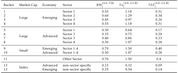
The required supervisory parameters for equity derivatives are set by BCBS (2014d). Table 1.1 shows the values for these regulatory prescribed parameters. According to BCBS (2013) the supervisory parameters (volatility, supervisory factor) for equities were calibrated using a three-step approach. First, the supervisory parameters were initially calibrated based on historic market data. These results were compared to a supervisory CCR model for different portfolio compositions. Finally, the supervisory authorities conducted a Quantitative Impact Study (QIS) to assess the impact of the calibrated SA-CCR on real-life portfolios.

14

For options with multiple exercise dates, one might only assume the latest exercise date.

15ψ

equals (

1) where the transaction is a sold call or a bought put option and (+1) where the transaction is a bought call or sold put option.

equals (

1) for put and (+1) for call options.

16

There are specific rules for the estimation of the respective inputs into the formula for exotic options (e.g. Asian, Bermudan, American, Digital). Nevertheless, there is no specification how to deal with Barrier options in the respective documents. Hence, we assume that SDA for Barrier options is calculated based on the simplified Black

& Scholes formula in equation (1.11).

17

Additional background on the calculation of the adjusted notional is available in APPENDIX 1.A.2.

18

A detailed description of aggregation methodologies is provided in BCBS (2014b).

Table 1.1: Supervisory parameters for equity derivatives

Risk Category Subclass SF

SF

b =σ

σ

ρ

Equity Index 6-10% 20% 75.2% 75% 80%

Equity Single-Name 6-10% 32% 120.3% 120% 50%

Notes: This table provides values for supervisory SA-CCR parameters as set by BCBS (2014d).

1.3 Regulatory status and discussions

In 2013, the BCBS issued a consultation paper on a new non-internal model method for calculating exposures for the capitalization of CCR exposures (BCBS (2013)). The final SA- CCR paper was published in 2014 (BCBS (2014d)). The transformation of the proposed new standardized approach into the regulatory capital framework di ff ers across jurisdictions in terms of content and timing. In Europe, the new requirements regarding the SA-CCR have been included in the new version of the Capital Requirements Regulation (EC (2019)). The mandatory compliance date is the 28th June 2021. In addition to the proposed approach, the European Commission introduced a simplified SA-CCR approach as well as a revised Original Exposure Method (OEM) to reduce the operational burden for institutions without material derivatives business. In late 2018, the responsible US agencies

published a proposed rulemaking for the implementation of the SA-CCR for consultation (OCC et al. (2018)). The final rule to implement the SA-CCR was issued in November 2019 together with details on industry responses and associated comments by the regulators (OCC et al. (2019)). The new rules will become effective as of 1st April 2020. The mandatory compliance date for “advanced approaches banking institutions“ was set to 1st January 2022.

Based on the proposed rulemaking, the US agencies collected about 58 responses from various stakeholders on different aspects of the SA-CCR methodology. In general, the agencies received broad endorsement for the implementation of the SA-CCR. Nevertheless, the commenters raised various concerns and suggestions for modifying the SA-CCR. Main areas of concerns are the application of the α-factor, the scheduled time-line for implementation as well as the overall level of conservatism resulting from the conservative design of the PFE multiplier, the overly conservative calibration of certain supervisory parameters and the lack of granularity of the supervisory parameters for some asset classes. In addition, there is ongoing discussion

19

The agencies involved in the rulemaking for SA-CCR are the Federal Deposit Insurance Corporation (FDIC), Department of Treasury - Office of the Comptroller of the Currency (OCC) and the Federal Reserve System (FED).

We will denominate those institutions as “US agencies“ in the course of this paper.