This paper suggests a fast and simple semi-analytical approach for exposure calculation, which is a modified version of the new regulatory standardized approach (SA-CCR)

(1)

https://doi.org/10.1007/s11147-019-09165-w

Computing valuation adjustments for counterparty credit risk using a modified supervisory approach

Patrick Büchel¹·Michael Kratochwil^2,3 ·Daniel Rösch²

Published online: 14 January 2020

Abstract

Considering counterparty credit risk (CCR) for derivatives using valuation adjustments (CVA) is a fundamental and challenging task for entities involved in derivative trading activities. Particularly calculating the expected exposure is time consuming and complex. This paper suggests a fast and simple semi-analytical approach for exposure calculation, which is a modified version of the new regulatory standardized approach (SA-CCR). Hence, it conforms with supervisory rules and IFRS 13. We show that our approach is applicable to multiple asset classes and derivative products, and to single transactions as well as netting sets.

Keywords Counterparty credit risk·Credit valuation adjustments (CVA)·Credit exposure·Standardized approach for measuring counterparty credit risk exposures (SA-CCR)

JEL Classification G21·G32

The authors would like to thank the participants of the Quantitative Methods in Finance (QMF) Conference 2018 in Sydney for helpful comments. We would also like to thank two anonymous referees for comments which greatly helped us improving the paper.

B Michael Kratochwil michael.kratochwil@ur.de Patrick Büchel

patrick.buechel@commerzbank.com Daniel Rösch

daniel.roesch@ur.de

1 Commerzbank AG, Mainzer Landstraße 157, 60327 Frankfurt am Main, Germany

2 Chair of Statistics and Risk Management, Universität Regensburg, Universitätsstraße 31, 93040 Regensburg, Germany

3 Dr. Nagler & Company GmbH, Maximilianstraße 47, 80538 Munich, Germany

(2)

1 Introduction

The financial crisis and its aftermath have revealed the importance of counterparty credit risk (CCR) in over-the-counter (OTC) derivative transactions. Today, the consideration of CCR is market standard and the calculation of credit valuation adjustments (CVA) has evolved to be a fundamental task for entities involved in derivatives trading due to several reasons. Firstly, market participants need to consider CCR when pricing derivatives. Secondly, international financial reporting standards (IFRS 13) require all entities involved in derivative transactions to consider CCR in the accounting fair value.¹Thirdly, financial institutions are expected to calculate minimum capital requirements for CVA risk under Basel III, which implies the calculation of CVA as well as CVA sensitivities. The most time-consuming and complex part of xVA calculation is the determination of the expected exposure. Given the lack of clear methodological guidance in IFRS 13, a wide range of methods has been developed by regulators, financial institutions and scientists alike. As many market participants may not be able to apply highly complex and sophisticated methods, there is a need for simpler semi-analytical and parametric approaches. Most existing approaches are either too simplistic to be robust, only applicable on transaction level or suitable for a small range of products. Hence, most of these methods are not applicable to multi- dimensional netting sets.

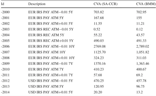
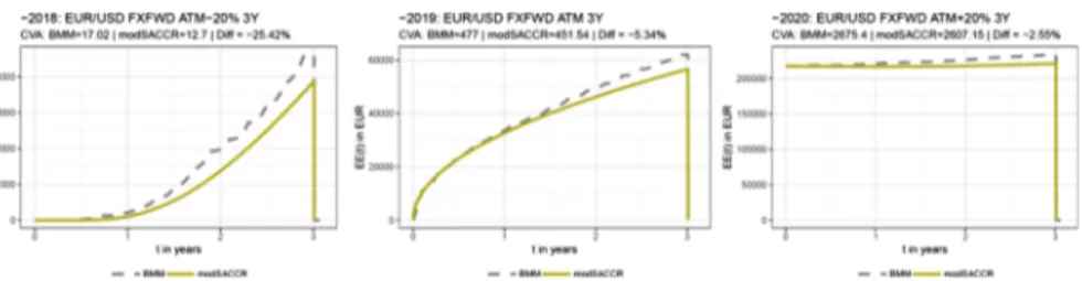
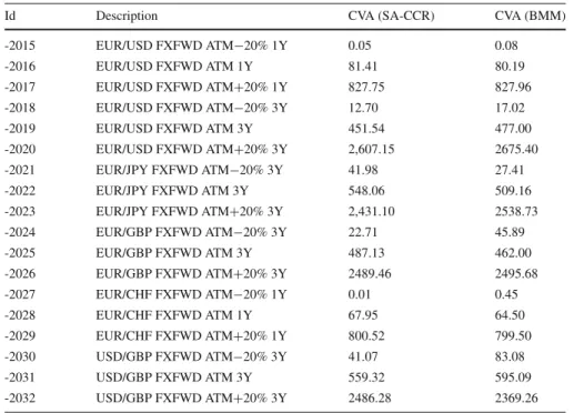
Our paper provides the following contributions. Firstly, we develop a fast and simple semi-analytical method for exposure calculation, which is a modified version of the new supervisory standardized approach for measuring counterparty credit risk exposures (SA-CCR). We derive the necessary adjustments to the regulatory SA-CCR in order to ensure consistency with IFRS 13. The approach has a flexible structure and is able to capture risk mitigating effects from margining and collateralization. Secondly, we show that our approach is applicable to multiple asset classes and on a single- transaction as well as a netting set level. To ensure the usability of our approach, we compare our results with an advanced model approach for an illustrative set of interest rate and foreign exchange derivatives.

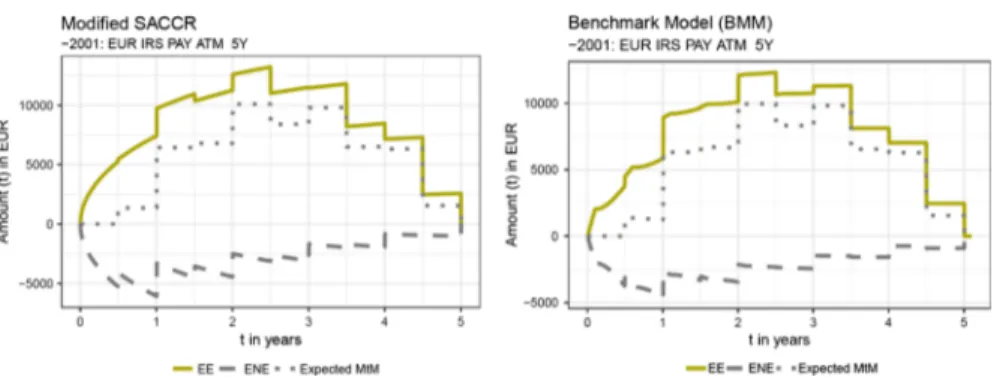
We find that our modified SA-CCR approach is able to produce expected exposure profiles capturing the main exposure dynamics of interest rate and foreign exchange positions. Hence, we are able to mirror exposure profiles generated by advanced methods, which might serve as input for CVA calculation. As we maintain the key building blocks and methodological assumptions of the supervisory SA-CCR, we offer a flexible and consistent approach to calibration based on market-implied volatilities, yet simple enough to be adopted by smaller institutions with limited personal resources.

The remainder of the paper is structured as follows. Section2provides an overview and categorization of existing methods for exposure quantification. In Sect.3we derive the necessary adjustments to the SA-CCR based on central model foundations. The calibration of the modified SA-CCR is lined out in Sect.4. The methodology and results of the empirical analysis are presented in Sect. 5. Section6 concludes this paper.

1 IFRS 13 also requires the inclusion of an entity’s own credit risk in the fair value measurement via the calculation of Debit Valuation Adjustments (DVA). In this paper we focus solely on the calculation of CVA based on the expected positive exposure. It is possible to adapt our approach for calculation of further xVAs.

(3)

2 Methods for exposure quantification

Calculation of xVAs requires the quantification of the expected exposure at timet. The lack of clear guidance from accountants and supervisors as well as the need for complex and simpler methods have led to the development of a wide range of approaches.

According to Gregory (2015), these methods can be divided into advanced, parametric and semi-analytical approaches. Using advanced approaches is the most sophisticated way to quantify CCR exposures, and there is plenty of academic literature on their application (see Pykhtin and Zhu2007; Pricso and Rosen2005; Picoult2004; Can- abarro and Duffie 2003; Picoult 2004). An advanced approach provides the most realistic risk assessment, but requires in-depth quantitative knowledge, a multitude of input data and a powerful infrastructure. Especially the simulation of potential market scenarios and the valuation of transactions for each scenario and viewpoint are complex and laborious tasks. Developing and maintaining an advanced model is complex and associated with high costs. While advanced approaches are usually applied in larger financial institutions, small and medium-sized market participants often do not have the capabilities to operate a complex exposure simulation model. Thompson and Dahinden (2013) find that even banks applying advanced models are often unable to cover all asset classes and products within these models. Therefore, we are certainly justified in saying that there is a need for alternative, less sophisticated approaches. To avoid an operational burdensome simulation model, various semi-analytical methods have been developed. These approaches are based on assumptions with respect to the development of risk factors driving the market value of a product or netting set. One prominent example for semi-analytical methods is the swaption approach introduced by Sorensen and Bollier (1994). They measure the exposure of an interest rate swap by valuing a series of swaptions, which a party would theoretically enter into in case of the counterparty’s default. There are several other semi-analytical methods for interest rate swaps and other derivative products (such as Leung and Kwok2005for credit default swaps). In the past years, there has been a lot of work on the development and enhancement of reduced-form and structural models for CVA calculation (e.g.

Kao2016; Hull and White2012; Cherubini 2013). While semi-analytical methods are considered the best choice for modelling CCR exposure on transaction level, their application is limited. Semi-analytical methods are generally suited for a limited number of products and designed for a specific asset class. Hence, it is difficult to apply these methods for products with multiple underlying risk factors (e.g. cross-currency- swaps) and multi-dimensional netting sets. In general, CCR exposures are calculated on netting set/counterparty level and require an aggregation of product-specific exposure profiles, which is something most of these semi-analytical methods are not able to provide. Most semi-analytical approaches ignore diversification and effects from collateralization, netting and margining. Even extensions are only able to recognize these effects in a very limited way. For example, Brigo and Masetti (2005) develop an analytical approach for interest rate portfolios in a single currency.

Parametric approachesare considered to be the most simplistic way of quantify- ing CCR exposures. They provide an approximation based on a limited number of simple parameters. Most parametric approaches calculate the exposure as the sum of current exposure (C E) and an add-on for potential future exposure (P F E). By

(4)

calibrating the aforementioned simple parameters to more complex methods, the out- come of parametric approaches is aligned with the results from more sophisticated models. Especially regulatory standardized approaches are based on the idea of sim- plification and calibration. When calculating the exposure at default (E A D) for the assessment of minimum regulatory capital requirements, banks currently have the option to choose between using an advanced Internal Model Method (IMM) or one of two standardized approaches (Standardized Method (SM), Current Exposure Method (CEM)).²According to EBA (2016) the Current Exposure Method (CEM) is the most widespread approach for calculating CCR exposures in the European banking sec- tor for regulatory purposes. This method was introduced by the Basel Committee on Banking Supervision (BCBS) (1996) and is still valid after it was adjusted in the course of Basel II (2005). A majority of financial institutions uses methods based on the CEM for accounting and pricing purposes. These approaches are often referred to as “mark-to-market plus add-on” methods. In the past, especially the CEM was criticized for several reasons. From the perspective of BCBS (2014c) the main issues are (1) the lack of risk sensitivity, (2) the outdated calibration of risk weights, (3) the missing ability to recognize credit risk mitigation techniques (in particular margining) as well as (4) a too simplistic attempt to capture netting effects.³

Driven by this criticism, the financial crisis and the increasing importance of bilateral margining in OTC derivatives markets,⁴a new regulatory standardized approach was developed by the BCBS (2014c). The SA-CCR will replace the existing standardized approaches (SM and CEM). With the development of the SA-CCR, the BCBS was striving for a holistic approach applicable to a variety of derivative products. Further- more, the SA-CCR was intended to overcome the weaknesses of existing approaches while keeping complexity on a reasonable level.

The SA-CCR can be classified as a semi-analytic method. It uses a rule based calculation scheme and simple parameters. Nevertheless, the derivation of the approach is based on detailed assumptions with respect to the distribution of market values and model based aggregation algorithms. The SA-CCR has several major advantages compared to its predecessors. First, the SA-CCR is able to distinguish between margined and unmargined netting sets. Effects of margining are considered in the current and potential future exposure component. This is an important feature in light of the rising importance of bilateral margining and central clearing. As stated in BCBS (2014c) the SA-CCR is also able to cope with complex situations (e.g. several netting sets are covered by one margin agreement). Second, the SA-CCR applies a more sophisticated approach to netting and diversification. This adds additional complexity, but should lead to higher risk sensitivity in the approximation of exposures (BCBS2014c). The

2 Institutions with very limited trading business have the possibility to use an even simpler method, the Original Exposure Method (OEM), for the purpose of calculating minimum regulatory capital requirements.

3 For a comprehensive discussion of critique of CEM, please refer to Fleck and Schmidt (2005) and Pykhtin (2014).

4 As a result of the global financial crises, regulators all over the world set regulations for reducing risk in the financial industry, especially in the OTC market, and to protect counterparties from the risk of a potential default of the other counterparty. These are the obligation to clear certain derivative products as well as the obligation to reduce the risk of non-cleared OTC derivative contracts by exchanging collateral in form of initial and variation margin (BCBS, IOSCO2015; ESAs2016).

(5)

structure of the calculation of potential future exposure is flexible and allows to add or delete elements where necessary.⁵Third, the SA-CCR takes over-collateralization, moneyness of transactions and the netting set into account. As excess collateral and transactions with negative values guard against rising exposures, this should lead to more realistic results. Overall, the SA-CCR is more complex compared to the popular CEM, but financial institutions might be able to leverage on the improved risk sensitivity and flexibility. The SA-CCR provides a consistent exposure calculation framework for all asset classes, while accounting for specific aspects of different financial products (such as equity options, swaptions, etc.). Considering these facts alongside the aforementioned improvements and the transparency with respect to its model foundations, the application of SA-CCR for CVA pricing and accounting purposes is an interesting option for all kinds of entities involved in derivatives trading.

According to Marquart (2016) the application of regulatory approaches (foremost CEM) is considered best practice when calculating exposures for CVA pricing. She analysed the impact on accounting CVA when switching from CEM to SA-CCR, under the assumption of using a simple CVA formulaC V A= P D·L G D·E A D, where E A Dis defined as the Effective Expected Positive Exposure (E E P E) resulting from SA-CCR, or CEM respectively. The application of the supervisory SA-CCR for CVA pricing compasses several issues. First, the SA-CCR aims for an approximation of the exposure at default (E A D) under the Internal Model Method (IMM). Under IMM, the E A Dis defined as the product of the Effective Expected Positive Exposure (E E P E) and a factor (α = 1.4), which is used to convert the E E P E into a loan equivalent exposure.⁶For CVA pricing, a time dependent expected exposure profile E E(t)is required. Hence, the target measure of the supervisory SA-CCR is not appropriate.

Second, the SA-CCR is calculated for a risk horizon of up to one year for unmargined netting sets. For the purpose of CVA pricing, an exposure profile for the life-time of a netting set is required. Using theE E P E orE A Das a scalar when calculating CVA would ignore the time dependency of exposure. Third, the SA-CCR is calibrated to a period of stress. This means resulting exposures are calculated under the real-world measure. According to IFRS 13, the calculation of CVA needs to be conform to the expectations of market participants. This requires a calibration under the risk-neutral measure. Additionally, the SA-CCR contains a set of conservative elements which should not be applied when calculating exposure for CVA pricing. In conclusion, we find that the SA-CCR in its supervisory form does not conform to IFRS 13. Hence, modifications to the regulatory SA-CCR are required to deploy the approach for CVA pricing and accounting purposes.

3 Derivation of the modified SA-CCR

This paper aims to define modifications to the supervisory SA-CCR to derive an approach for the calculation of expected exposure profiles. As stated above, the adjust-

5 There are discussions to give national competent authorities the option to adjust the add-on structure for institutions with complex commodity trading activities.

6 For information on the calibration and theoretical background ofα, please refer to ISDA, TBMA, LIBA (2003), Lynch (2014) and Gregory (2015).

(6)

ments are necessary in order to calculate exposure values suitable for CVA calculations.

While adjusting the SA-CCR, we aim to retain the basic structure and main building blocks. This allows the application of a consistent approach across asset classes and enables financial institutions to leverage on future implementations of the supervisory SA-CCR. The following presentation of the SA-CCR methodology and the derivation of its adjustments is based on the content and structure of BCBS (2014b).

The calculation of CVA requires an expected exposure profile as the main input. In the absence of collateral, the expected exposure of a netting set (k) is defined as the expected positive value of the netting set’s market value (Vk) at a future point in time (t):

E Ek(t)=IE^Q[max(Vk(t),0)] (1) In its supervisory form, the target measure of the SA-CCR is a conservative Effective Expected Positive Exposure (E E P E) on netting set level under the real-world measure (calibrated to historic stressed volatilities). Hence, the main adjustment when deriving our approach is the change of target measure to an E Ek(t)under the risk-neutral measure. To retain the general structure of the SA-CCR, we define E Ek(t)as the combination of replacement costs (RCk(t)) and potential future exposure (P F Ek(t)):

E Ek(t)=RCk(t)+P F Ek(t) (2) Please note that both components of the modified SA-CCR are a function of time (t).

Following our approach,RCk(t)captures the deterministic component, while potential future exposure quantifies the stochastic component ofE Ek(t). In the following sections, we derive the modified formulas for calculation of these components on netting set level. Finally, we transfer our results to the SA-CCR specific parameters for exposure calculation.

3.1 Replacement costs

For the derivation of the replacement costs formula, we first introduce the following assumptions.(A1)A transaction’s market value follows a driftless brownian motion.

For the formulation of replacement costs, we set the volatility to zero. (A2) We assume no cash flows between (t0,t). (A3) Furthermore, the transaction’s netting set is unmargined and therefore not supported by a margin process.⁷These assumptions are used implicitly by BCBS (2014b) for the derivation of RC for unmargined netting sets.

Under these assumptions, the future market value of a transaction (Vi) at a specific point in time (t) is defined as:

Vi(t)=Vi(t0)+σi(t)·√

t·Xi (3)

7 A netting set is considered to be unmargined if there is no exchange of variation margin (V M). Never- theless, other types of collateral (such as initial margin (I M)) might be present.

(7)

where Vi(t0)represents today’s market value and Xi is a standard normal random variable (Xi ∼ N(0,1)).σi(t)represents the volatility of the transaction’s market value at timet. Applying assumptionA1, the expected future market value is equal to today’s market value as the second term of Eq. (3) becomes zero. As stated above, RC(t)should capture the deterministic movements of a transaction’s market value. In particular, interest rate and credit default swaps involve regular payments resulting in a change of the transaction’s market value over time. In order to cover these deterministic effects, we relax assumption A2. Given assumptionA1, the future market value of a transaction is deterministic and can be calculated based on the transaction’s future cash flows. This may generally be written as:

Vˆi(t)= T

j=t

C FR EC(tj)·D F(t,tj)− T

j=t

C FP AY(tj)·D F(t,tj) (4)

where C FR EC(tj)is the cash flow received at timetj,C FP AY(tj)equals the cash flow paid at timetj andD F(t,tj)represents the discount factor from timetj to time t.

For more complex derivatives or in case no information regarding future cash flows is available, we introduce a time-dependent and product specific scaling factor (si) to provide an approximation of the future market value of a transaction (Vˆi(t)).

Vˆi(t)=Vi(t0)·si(t) (5) For interest rate or credit default swaps, this scaling factor might be based on a sim- plified duration measure for the respective product:

si(t)= Di(t)

Di(t0)·1_{Mi≥t} (6) where 1_{Mi≥t}is an indicator variable which has the value of 1 if the transaction has not expired att (i.e., maturity Mi is greater or equal thant). The duration measure Di(t)is defined as:⁸

Di(t)= exp(−r·max(Si,t))−exp(−r·Ei)

r (7)

where Si is the start date of the transaction and Ei its end date.r is defined as the current interest rate level. For simple products in other asset classes,s_i⁽^a⁾ could be represented by the indicator variable. Nevertheless, our approach offers the flexibility to define a transaction specific scaling factor for all kinds of (exotic) products. This allows a recognition of deterministic developments of the transaction’s market value in a flexible and consistent setting.

Within a legally enforceable netting set (k), the offsetting between transactions with positive and negative market values (Vˆi(t)) is allowed. Hence, a netting set’s market value at timetis defined as:

8 For the derivation ofD_i(t)please refer to “AppendixA.3.3”.

(8)

Vˆk(t)=

i∈k

Vˆi(t) (8)

As stated above, replacement costs do not involve stochastic elements. Thus, the expectation of the future market value is solely driven by deterministic movements and hence represented byVˆk(t). This leads to the following formulation of replacement costs for unmargined and uncollateralized netting sets:

RCk(t)=IE^Q[max(Vk(t),0)]=max

Vˆk(t),0

(9) In the presence of collateral, the market value of the netting set is reduced by the cash-equivalent value of net collateral received (CC E(t)). Under assumptionA3, all collateral posted or received has the form of independent collateral. Given the lack of a margin process, no adjustment to the notional amount of collateral posted/received is required. The time dependency of the collateral value is limited to the volatility of the collateral value itself. In accordance with the supervisory SA-CCR, we calculate cash- equivalent values of collateral (CC E(t)) using collateral haircuts. There are two main adjustments to the supervisory approach. Firstly, we do not use a fixed time horizon, but calculate the cash-equivalent value for specific points in time (t). Secondly, we do not apply regulatory prescribed haircuts, but values based on institutions’ own volatility estimates. Given these adjustments,CC E(t)is defined as:

CC E(t)=

c∈k

V_c^{r ec}(t0)·(1−hc(t))−

c∈k

Vc^post^,^unseg(t0)·(1+hc(t)) (10)

where Vc equals the market value of a received (V_c^{r ec}(t0)) or unsegregated posted (Vc^post^,^unseg(t0)) collateral position at timet=t0. The haircut applicable to a specific collateral position is represented byhc(t). Please note that segregated posted collateral is not relevant for the calculation of replacement costs, as it is placed in a bankruptcy remote account and will therefore not increase exposure to the relevant counterparty.

Including collateral positions in the calculation of replacements costs for unmargined netting sets leads to:

RCk(t)=max

Vˆk(t)−CC E(t),0

(11) In order to derive a formulation for margined netting sets, we need to relax assumption A3. Within the modified SA-CCR, we introduce the possibility to model collateral dynamics directly. We calculate the future expected market value of each transaction at each point in timetbased on known cash flows using Eq. (4) or by applying a scaling factor (see Eq. (5)). Hence, we know the expected future market value of the netting set (Vˆk(t)) at eacht. Based on this information, we are able to derive an expected collateral path including the consideration of margin parameters like threshold (T H) and Minimum Transfer Amount (M T A). In case of (T H = 0) collateral is only exchanged, when the threshold is exceeded. This implies that the incremental amount above the threshold is exchanged in form of collateral. We define the amount above

(9)

the threshold as the collateral demand (CˆD(t)). If (M T A = 0), collateral is only exchanged, when the absolute difference between the current collateral position (Cˆ(t)) and the collateral demand exceeds the M T A. Under the assumption of symmetric M T AandT H, absence of rounding, daily margining and instantaneous processing of collateral exchange, the expected collateral position attjis defined as:⁹

C(tˆ j)= ˆC(tj−1)+max

max

CˆD(tj)− ˆC(tj−1),0

−M T A,0 +mi n

mi n

CˆD(tj)− ˆC(tj−1),0

+M T A,0

(12) where the collateral demand (CˆD(t)) is defined as:

CˆD(tj)=max

max

Vˆ(tj),0

−T H,0 +mi n

mi n

Vˆ(tj),0

+T H,0

(13) Based on this definition, the replacement costs for a margined netting set at t are defined as:¹⁰

RC_k^{mar gi n}(t)=max

Vˆk(t)− ˆC(t)+N I C A,0

(14) whereN I C Arepresents the Net Independent Collateral Amount defined as:

N I C A=I Mr ec−I M^unseg_post (15) In addition to modelling collateral dynamics directly, we introduce an optional (alternative), more simplistic approximation for the recognition of collateral in margined netting sets. This conservative approximation follows the methodology described in BCBS (2014b). We assume that the latest exchange of variation margin is not known at timet. Hence, we estimateRC(t)of margined netting sets as the maximum of replacement costs of an equivalent unmargined netting set, the highest exposure amount which would not trigger a margin call and zero. In general, a margin call is triggered if the uncollateralized market value is equal to the sum ofT H andM T A. This amount is reduced by the net independent collateral amount (N I C A).¹¹

Under a margin agreement, changes in the netting set’s market value will lead to changes in the amount of variation margin posted or received. Therefore, we introduce a time-dependent adjustment for variation margin (V M) based on the change of the market value of the netting set. Based on this adjustment, we arrive at the following

9 Please note that our approach offers the possibility to integrate additional collateral parameters, such as independent amounts, rounding or other re-margining periods.

10 Please note that the application of haircuts is also required for margined netting sets. In case of a margined netting set, the risk horizon for the application of haircuts is set to the MPOR.

11 In this caseN I C Ahas to include differential of the independent amounts used as parameters within the calculation of variation margin amounts.

(10)

approximation of replacement costs for margined netting sets:

RC_k^{mar gi n}(t)≈max

Vˆk(t)− ˆCC E(t),T H+M T A−N I C A,0

(16) whereCˆC E(t)is defined as:

CˆC E(t)=

c∈k

V_c^{V M}(t0)·(1±hc(M P O R))

· Vˆk(t)

Vk(t0)+N I C A (17) where V_c^{V M}(t0)is defined as today’s market value of a variation margin collateral position.¹²In general we cap the expected exposure of a margined netting set at the expected exposure of an equivalent netting set without any form of margin agreement.

This is equal to the assumption that a netting set is treated as unmargined as long as no collateral is exchanged (e.g. the sum of MTA and TH is not exceeded).. This procedure is required to avoid overly conservative results due to high thresholds and minimum transfer amounts.

3.2 Potential future exposure

In line with BCBS (2014b) we define the potential future exposure (P F E) as the product of a multiplier (mk) and an aggregated add-on (Add Onk) for each netting set (k):

P F Ek(t)=mk(t)·Add Onk(t) (18) wheremk(t)is a function ofCˆC E(t),Vˆk(t)as well as the calculated aggregated add-on (Add Onk(t)) of the respective netting set (k). In our approach, the aggregated add- on represents an analytical approximation of E Ek(t)on netting set level, assuming a market value of zero and the absence of collateral. The multiplier is introduced to account for market value and collateral amounts different from zero. The regulatory SA-CCR approach reflects the benefit of excess collateral and negative market values, as only these are mitigants against potential future exposure. Please note that the multiplier as well as the aggregated add-on are a function of time (t). In the subsequent paragraphs we provide the derivation of add-ons as well as the multiplier formula.

3.2.1 Add-ons for unmargined netting sets

The netting set level add-on for unmargined netting sets represents an estimate of the expected exposure (E E) at timet. The assumptions of the regulatory SA-CCR presented in BCBS (2014b) are maintained in order to build a consistent and integrated framework. Hence, our approach is based on the following main assumptions:

12 Please note that a change in sign ofVˆ_k(t)will also lead to a change in sign of variation margin. In case of posted VM, segregated collateral needs to be eliminated from the calculation ofCˆ_{C E}(t). Hence, assumptions on the properties of potentially posted and received variation margin are required.

(11)

– AO1:The market value of all transactions is zero (Vi(t)=0). This assumption implies that the market value of the netting set is zero (Vk(t)=0).

– AO2:There is neither received nor posted collateral (CC E(t)=0).

– AO3:There are no cash-flows within the time period(t0,t)

– AO4:The evolution of each transaction’s market value follows an arithmetic brownian motion with zero drift.

Under these assumptions, the expected exposure of a netting set at timet is defined as:¹³

E Ek(t)=IE^Q[max(Vk(t),0)]=IE^Q

max(σk(t)·√

t·Y,0)

(19) withσk(t)representing the annualized volatility of the netting set’s market value att.

AsY is a standard normal variable, we can calculateE Ek(t)analytically. Hence, the expected exposure solves for:¹⁴

E Ek(t)=σk(t)·√

t·φ(0) (20)

whereφ(0)is defined as the standard normal probability density:φ(0)= 1/√ 2π.

According to BCBS (2014b) and in line with the above foundations, we are able to restate this equation at trade level in order to calculate an expected exposure at trade levelE Ei(t).

Add Oni(t)=E Ei(t)=σi(t)·√

t·φ(0) (21)

Please note that contrary to BCBS (2014b) the volatility of the market value on trade level (σi(t)) is a function oftas we estimate the volatility of each transaction’s market value as a function oft. Nevertheless, we are generally able to use the same structure and aggregation methodology for the calculation of add-ons as proposed by BCBS (2014b).¹⁵

3.2.2 Add-ons for margined netting sets

The add-on for margined netting sets aims to estimate the expected increase of exposure between time of default (τ = t) and the final close-out of positions (t+M P O R).

Given assumptionsAO1,AO2andAO3and in accordance with the argumentation of BCBS (2014b), the calculation of this amount on netting set level can be reduced to:

Add On^{mar gi n}_k (t)=E E^{mar gi n}_k (t)=σk(t)·φ(0)·√

M P O R (22)

13 For detailed derivation of Eq. (19), please refer to “AppendixA.1”.

14 For the respective derivation of the analytical formulation ofE E_k(t), please refer to “AppendixA.1”.

15 The validity of this assumption under the new target measureE E(t)is proven in “AppendixA.2”.

(12)

For a netting set with only one trade, we can restate formula (22) and arrive at the formulation for the trade-level add-on for transactions in a margined netting set.¹⁶

Add On^{mar gi n}_i (t)=σi(t)·φ(0)·√

M P O R (23)

3.2.3 Structure of add-on calculations

The regulatory SA-CCR has a specific structure for the calculation of PFE add-ons.

Aggregation procedures are used to calculate netting set level add-ons from trade- level add-ons. These aggregation rules are based on the central idea that add-ons can be aggregated like standard deviations. While deriving our modified approach for add- on calculation, we apply similar assumptions as used for developing the regulatory SA-CCR. We have shown that the general principles of the SA-CCR are still valid under the new target measure (E E(t)). Hence, we are generally able to apply the same basic structure and methodology for aggregation as provided by the regulatory SA-CCR.

The first step for calculating the aggregated add-on on netting set level is the determination of an add-on at trade-level. In line with the regulatory SA-CCR, the calculation of trade-level add-ons is asset class specific, but has common features for all derivative transactions. Hence, each transaction is allocated to at least one of five asset classes based on the primary risk factor.¹⁷ For products with more than one material risk factor, the assignment to multiple asset classes is required.¹⁸

Following the supervisory SA-CCR, we operate with simple trade-level parameters instead of trade-level volatilities (σi(t)) directly. Hence, we define a transaction’s add- on at timet as the product of an exposure factor (E Fi), the adjusted notional amount (di), its delta (δi) and a scaling factor with respect to time (√

t or√

M P O R).¹⁹ Add Oni(t)=E Fi·di(t)·δi(t)·√

t (24)

Add On^{mar gi n}_i (t)=E Fi·di(t)·δi(t)·√

M P O R (25)

By inserting Eq. (21) into Eq. (24) and solving forσi(t), we arrive at the following approximation for the volatility of the transaction’s market value att:

σi(t)= E Fi

φ(0)·di(t)· |δi(t)| (26)

16 As shown in “AppendixA.2”, the aggregation of trade-level add-ons also holds true when aggregating margined trade-level add-ons.

17 Within this paper we share the number and set-up of asset classes and hedging sets proposed by the Basel Committee. Nevertheless, the general structure of our approach allows for further modification with respect to the amount and definition of asset classes, hedging and subsets.

18 Details with respect to this requirement are still under discussion. A first discussion paper has been published by EBA (2017).

19 The maturity factor (M F_i) used in the supervisory SA-CCR is applied as correction for trades maturing within the risk horizon of 1 year for unmargined netting sets. Under the target measureE E(t), this is not necessary, as no averaging over a dedicated risk horizon is applied. Hence, a maturity factor is not required.

(13)

In accordance with BCBS (2014b) the ratio ofE Fi andφ(0)can be interpreted as the annualized standard deviation of the transaction’s primary risk factor (σ_i⁽^{R F}⁾):

σ_i⁽^{R F}⁾= E Fi

φ(0) (27)

Please note that the volatility of the risk factor (σ_i⁽^{R F}⁾) is assumed to be constant over time. Hence, the time dependence of the volatility of the transaction’s market value is solely resulting fromdi(t)andδi(t). The exposure factor (E Fi) can be interpreted as an approximation of the expected exposure of a netting set with one directional trade, which has the size of one unit adjusted notional att =1year.

E Fi =σ_i⁽^{R F}⁾·φ(0) (28) This relationship allows a calibration ofE Fi based on the (implied) volatility of the transaction’s primary risk factor (σ_i⁽^{R F}⁾). The supervisory SA-CCR provides supervisory factors (S Fi) on subclass level.²⁰We introduce a more granular approach to the calibration of the exposure factor in Sect.4.

Thedelta parameter(δi) is a function of the direction of the trade with respect to the primary risk factor (long / short). For products with a non-linear relationship to the primary risk factor,δi serves as a scaling factor with respect to the moneyness of the product.²¹For plain vanilla options we use a delta formula based on the formula provided by the supervisory SA-CCR (BCBS2014c):

δi(t)=ψ·N

⎛

⎜⎝ω·ln(P(t)/Kˆ )+0.5·

σ_i⁽^{i mpl}⁾2

·(T −t) σ_i⁽^{i mpl}⁾

·√ (T −t)

⎞

⎟⎠ (29)

whereKrepresents the strike price andσ_i⁽^{i mpl}⁾the (implied) volatility of the underlying of the option.Tis defined as the amount of time (in years) between today and the expiry date of the option.²² P(tˆ )equals an estimation of the spot price of the underlying at timet.²³ If an estimation of P(t)via the forward price is not possible, we assume P(t) = P(t0). The parametersψ andωare required to cover all combinations of bought/sold and call/put options.²⁴

For more complex and exotic options Eq. (29) might not be appropriate as a lot of these products are path-dependent. Asδi(t)is defined on trade-level, our approach

20 Such as rating categories within asset class credit.

21 Please note that supervisory approach is offering a specific delta formula for CDOs which uses detach- ment and attachment points as inputs for the calculation of the delta parameter.

22 For options with multiple exercise dates, one might only assume the latest exercise date.

23 Example: For FX options, we are able to estimate the forward price at timetbased on the interest rate curves of the involved currencies.

24 ψequals(−1)where the transaction is a sold call option or a bought put option and sign(+1)where the transaction is a bought call option or sold put option.ωequals(−1)for put and(+1)for call options.