Cointegrating Polynomial Regressions: Fully Modified OLS Estimation and Inference

IHS Economics Series Working Paper 264

March 2011

Cointegrating Polynomial Regressions: Fully Modified OLS Estimation and Inference

Seung Hyun Hong

Martin Wagner

Impressum Author(s):

Seung Hyun Hong, Martin Wagner Title:

Cointegrating Polynomial Regressions: Fully Modified OLS Estimation and Inference ISSN: Unspecified

2011 Institut für Höhere Studien - Institute for Advanced Studies (IHS) Josefstädter Straße 39, A-1080 Wien

E-Mail: o ce@ihs.ac.at ffi Web: ww w .ihs.ac. a t

All IHS Working Papers are available online: http://irihs. ihs. ac.at/view/ihs_series/

This paper is available for download without charge at:

https://irihs.ihs.ac.at/id/eprint/2047/

Cointegrating Polynomial Regressions:

Fully Modified OLS Estimation and Inference

Seung Hyun Hong, Martin Wagner

264

Reihe Ökonomie

Economics Series

264 Reihe Ökonomie Economics Series

Cointegrating Polynomial Regressions:

Fully Modified OLS Estimation and Inference

Seung Hyun Hong, Martin Wagner March 2011

Institut für Höhere Studien (IHS), Wien

Institute for Advanced Studies, Vienna

Contact:

Seung Hyun Hong

Korea Institute of Public Finance Seoul, Korea

Martin Wagner

Department of Economics and Finance Institute for Advanced Studies Stumpergasse 56

1060 Vienna, Austria Vienna, Austria

: +43/1/599 91-150 fax: +43/1/599 91-555 email: mawagner@ihs.ac.at and

Frisch Centre for Economic Research Oslo, Norway

Founded in 1963 by two prominent Austrians living in exile – the sociologist Paul F. Lazarsfeld and the economist Oskar Morgenstern – with the financial support from the Ford Foundation, the Austrian Federal Ministry of Education and the City of Vienna, the Institute for Advanced Studies (IHS) is the first institution for postgraduate education and research in economics and the social sciences in Austria. The Economics Series presents research done at the Department of Economics and Finance and aims to share “work in progress” in a timely way before formal publication. As usual, authors bear full responsibility for the content of their contributions.

Das Institut für Höhere Studien (IHS) wurde im Jahr 1963 von zwei prominenten Exilösterreichern –

dem Soziologen Paul F. Lazarsfeld und dem Ökonomen Oskar Morgenstern – mit Hilfe der Ford-

Stiftung, des Österreichischen Bundesministeriums für Unterricht und der Stadt Wien gegründet und ist

somit die erste nachuniversitäre Lehr- und Forschungsstätte für die Sozial- und Wirtschafts-

wissenschaften in Österreich. Die Reihe Ökonomie bietet Einblick in die Forschungsarbeit der

Abteilung für Ökonomie und Finanzwirtschaft und verfolgt das Ziel, abteilungsinterne

Diskussionsbeiträge einer breiteren fachinternen Öffentlichkeit zugänglich zu machen. Die inhaltliche

Verantwortung für die veröffentlichten Beiträge liegt bei den Autoren und Autorinnen.

Abstract

This paper develops a fully modified OLS estimator for cointegrating polynomial regressions, i.e. for regressions including deterministic variables, integrated processes and powers of integrated processes as explanatory variables and stationary errors. The errors are allowed to be serially correlated and the regressors are allowed to be endogenous. The paper thus extends the fully modified approach developed in Phillips and Hansen (1990). The FM-OLS estimator has a zero mean Gaussian mixture limiting distribution, which is the basis for standard asymptotic inference. In addition Wald and LM tests for specification as well as a KPSS-type test for cointegration are derived. The theoretical analysis is complemented by a simulation study which shows that the developed FM-OLS estimator and tests based upon it perform well in the sense that the performance advantages over OLS are by and large similar to the performance advantages of FM-OLS over OLS in cointegrating regressions.

Keywords

Cointegrating polynomial regression, fully modified OLS estimation, integrated process, testing

JEL Classification

C12, C13, C32

Comments

The helpful comments of Peter Boswijk, Robert Kunst, Benedikt M. Pötscher, Martin Stürmer, Timothy

J. Vogelsang, of seminar participants at Helmut Schmidt University Hamburg, University of Linz,

University of Innsbruck, Universitat Autònoma Barcelona, University of Tübingen, Tinbergen Institute

Amsterdam, Korea Institute of Public Finance, Bank of Korea, Korea Institute for International

Economic Policy, Korea Securities Research Institute, Korea Insurance Research Institute, Michigan

State University, Institute for Advanced Studies and of conference participants at the 2nd International

Workshop in Computational and Financial Econometrics in Neuchâtel, an ETSERN Workshop in

Copenhagen, the 3rd Italian Congress of Econometrics and Empirical Economics in Ancona, the

Econometric Study Group Meeting of the German Economic Association, the Econometric Society

European Meeting in Barcelona, the Meeting of the German Economic Association in Magdeburg and

the Statistische Woche in Nuernberg are gratefully acknowledged. Furthermore, we would like to thank

in particular the co-editor, the associate editor and two anonymous referees for their extremely valuable

comments and suggestions. The usual disclaimer applies.

Contents

1 Introduction 1

2 Theory 4

2.1 Setup and Assumptions ... 4

2.2 Fully Modified OLS Estimation ... 8

2.3 Specification Testing based on Augmented and Auxiliary Regressions ... 11

2.4 KPSS Type Test for Cointegration ... 15

3 Simulation Performance 17

4 Summary and Conclusions 26

References 28

Appendix A: Proofs 33

Appendix B: Modified Bonferroni Bound Tests, the Minimum Volatility Rule and Critical Values for CS Test

(Supplementary Material) 39 Appendix C: Additional Simulation Results

(Supplementary Material) 41

1 Introduction

This paper develops a fully modified OLS (FM-OLS) estimator for cointegrating polynomial regres- sions (CPRs), i.e. for regressions including deterministic variables, integrated processes and integer powers of integrated processes as explanatory variables and stationary errors. As in the standard cointegration literature the errors are allowed to be serially correlated and the regressors are allowed to be endogenous.

Thus, the paper extends the FM-OLS estimator of Phillips and Hansen (1990) from cointegrating (linear) regressions to cointegrating polynomial regressions. A major advantage of considering regressions of the considered form is that they are linear in parameters, which implies that linear least squares based estimation methods can be developed and that it is not necessary to consider nonlinear estimation techniques that require numerical optimization procedures. Clearly, the considered class of functions is restrictive, despite the fact that polynomials can be used to approximate more general nonlinear functions, but clearly this restriction is the price to be paid for having a simple linear least squares based estimation technique available (see Section 2.1 for further discussion). Additionally also specification and cointegration tests are developed. With respect to specification testing amongst other things this paper extends the work of Hong and Phillips (2010), who consider LM-type specification testing based on residuals of cointegrating linear relationships, in several aspects (see Section 2.3). With respect to asymptotic theory our work relies upon im- portant contributions of Chang, Park, and Phillips (2001), Park and Phillips (1999, 2001) and Ibragimov and Phillips (2008).

One motivation for considering CPRs is given by the so-called environmental Kuznets curve (EKC) hypothesis, which postulates an inverse U-shaped relationship between measures of economic ac- tivity (typically proxied by per capita GDP) and pollution. The term EKC refers by analogy to the inverted U-shaped relationship between the level of economic development and the degree of income inequality postulated by Kuznets (1955) in his 1954 presidential address to the Ameri- can Economic Association. Since the seminal work of Grossmann and Krueger (1995) more than one-hundred refereed publications (as counted already several years ago by Yandle, Bjattarai, and Vijayaraghavan, 2004) perform econometric analysis of EKCs.

Many of these empirical studies use unit root and cointegration techniques and include as regressors powers of per capita GDP (in

1

The theory is developed to allow also for predetermined stationary regressors, which are neglected from the discussion here for the sake of brevity. They are included in the discussion in Hong and Wagner (2008).

2

In addition to the vast empirical literature there is also a large theoretical literature exploring different mechanisms

leading to EKC type relationships, see e.g. the survey Brock and Taylor (2005).

order to allow to for U- or inverted U-shaped relationships). This literature neglects throughout that powers, as special cases of nonlinear functions, of integrated processes are not themselves in- tegrated processes, which invalidates the use of standard unit root and cointegration techniques.

Such relationships – in our terminology cointegrating polynomial relationships – necessitate the development of appropriate estimation and inference tools, which is done in this paper. For a more detailed discussion of the empirical EKC literature, its problems as well as a detailed analysis using the methods developed in this paper see Hong and Wagner (2008, 2010). A second strand of the empirical literature that can benefit from the theory developed in this paper is the so-called inten- sity of use literature that investigates the potentially also inverted U-shaped relationship between GDP and energy or metals use (see e.g. Labson and Crompton, 1993).

As in standard cointegrating regressions, the OLS estimator is consistent also in CPRs. Also as in the standard case, its limiting distribution is contaminated by so-called second order bias terms in case of error serial correlation and/or endogeneity of regressors (see the original work of Phillips and Hansen, 1990). This renders valid inference difficult. Consequently, we develop an FM-OLS estimator, which extends the FM-OLS estimator of Phillips and Hansen (1990) to CPRs, that has a zero mean Gaussian mixture limiting distribution and thus allows for standard asymptotic chi- square inference. The zero mean Gaussian mixture limiting distribution of the FM-OLS estimator also forms the basis for specification testing based on augmented (Wald tests) respectively auxiliary (LM tests) regressions. On top of these specification tests we also consider a KPSS-type test as a direct test for nonlinear cointegration of the considered form. The asymptotic distribution of this test depends on the specification of the deterministic components as well as the number and powers of integrated regressors included. This test extends the cointegration test of Shin (1994) from cointegrating to cointegrating polynomial regressions. We furthermore follow Choi and Saikkonen (2010) and consider also a sub-sample test that can be used in conjunction with the Bonferroni bound and which has a limiting distribution independent of the specification.

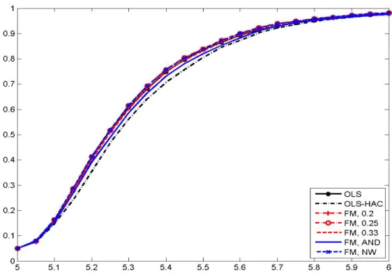
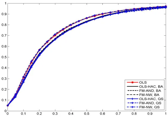
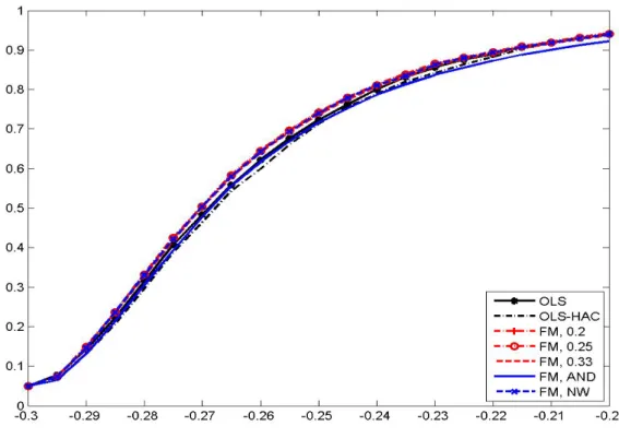
The theoretical analysis of the paper is complemented by a simulation study to assess the perfor-

mance of the estimator and tests, with the performance being benchmark against results obtained

by applying OLS. Many of the findings with respect to both estimator performance (measured in

terms of bias and RMSE) as well as the performance of the coefficient tests (size distortions, size

corrected power) are similar as for FM-OLS in standard cointegrating relationships. Summarized

in one sentence: the larger the extent of serial correlation and/or regressor endogeneity, the bigger

are the performance advantages of the FM-OLS estimator and test statistics based upon it. For

sizeable serial correlation and endogeneity the bias can be reduced by about 50% when using the FM-OLS instead of the OLS estimates and the over-rejections that occur for the FM-OLS based tests are less than half as big as for OLS based statistics. The choice of kernel and bandwidth is of relatively minor importance. With respect to the specification tests it turns out that the Wald tests are outperformed by the LM tests, since the latter have essentially the same, or for small sample sizes slightly lower, size corrected power but much smaller over-rejections under the null hypothesis than the former. The simulations also show that using as additional regressors both higher order deterministic trends (originally considered in a unit root and cointegration test context by Park and Choi, 1988; Park, 1990) together with higher polynomial powers of integrated regressors leads to highest power against the variety of alternatives considered. In the simulations the performance of the KPSS-type tests is rather poor. As is well known for KPSS-type tests, their performance is detrimentally affected by the presence of serial correlation, which is also confirmed by our simula- tions. The sub-sample test suffers additionally from the conservativeness of the Bonferroni bound and performs worse than the full sample test.

The paper is organized as follows. In Section 2 we derive the asymptotic results for the estimators and tests. Section 3 contains a small simulation study to assess the finite sample performance of the proposed methods and Section 4 briefly summarizes and concludes. The proofs of all propositions are relegated to the appendix. Available supplementary material contains further results in relation to the sub-sample KPSS-type test as well as additional simulation results.

We use the following notation: Definitional equality is signified by := and ⇒ denotes weak conver- gence. Brownian motions, with covariance matrices specified in the context, are denoted with B(r) or B . For integrals of the form ∫

0

B (s)ds and ∫

0

B(s)dB(s) we use short-hand notation ∫

B and

∫ BdB. For notational simplicity we also often drop function arguments. With ⌊ x ⌋ we denote the integer part of x ∈ R and diag(·) denotes a diagonal matrix with the entries specified throughout.

For a square matrix A we denote its determinant with | A | , for a vector x = (x

) we denote by

|| x ||

= ∑

i

x

and for a matrix M we denote by || M || = sup

. E denotes the expected value

and L denotes the backward-shift operator, i.e. L { x

}

= { x

}

.

2 Theory

2.1 Setup and Assumptions

We consider the following equation including a constant and polynomial time trends up to power q (see the discussion below), integer powers of integrated regressors x

, j = 1, . . . , m up to degrees p

and a stationary error term u

:

y

= D

θ

+

∑

X

θ

+ u

, for t = 1, . . . , T, (1) with D

:= [1, t, t

, . . . , t

]

, x

:= [x

, . . . , x

]

, X

:= [x

, x

, . . . , x

]

and the parameter vectors θ

∈ R

and θ

∈ R

. Furthermore define for later use X

:= [X

, . . . , X

]

, Z

:= [D

, X

]

and p := ∑

j=1

p

. In a more compact way we can rewrite (1) as

y = Dθ

+ Xθ

+ u (2)

= Zθ + u,

with y := [y

, . . . , y

]

, u := [u

, . . . , u

]

, Z := [D X] and θ = [θ

θ

]

∈ R

and

D :=



  D

.. . D



  ∈ R

, X :=



  X

.. . X



  ∈ R

.

Equation (1) is referred to as cointegrating polynomial regression (CPR). Clearly it is a special case of a nonlinear cointegrating relationship as considered in the literature (for recent examples see e.g. Karlsen, Myklebust, and Tjostheim, 2007; Wang and Phillips, 2009) where typically any relationship of the form y

= f(x

, θ) + u

, with x

an integrated process, u

stationary and f ( · , · ) a nonlinear function, is considered to be a nonlinear cointegrating relationship between y

and x

.

The econometric literature has not yet provided definite answers to the problem of how to extend the concepts of integrated and cointegrated processes, which are concepts inherently related to linear processes, to the nonlinear world. In the formulation just given, e.g. a minimum requirement for a useful extension of the concept clearly is to exclude cointegration in x

, since otherwise (this example

3

Any such formulation by construction treats

and

asymmetrically, with the former being a function (up

to

) of the latter which is assumed to be integrated in the ‘usual’ sense of the word. In the linear cointegration

framework, under the assumption that there is no cointegration between the components of

, this implies that in a

triangular system of the form

=

+

,

=

+v

also

is integrated and thus this asymmetric formulation

is innocuous. In a nonlinear framework the stochastic properties of

are in general unclear, when

is generated

by

=

(x

,

=

+

.

is taken from Choi and Saikkonen, 2010) a nonlinear function of the form f (x

, θ) = x

θ + (x

θ)

, with θ a cointegrating vector of x

, would lead to meaningless forms of nonlinear cointegration (some simple examples are also discussed in Granger and Hallman, 1991). The appeal of certain types of nonlinear functions to be used in nonlinear cointegration analysis, stems from the implied stochastic properties of f(x

, θ) and consequently of y

. In this respect the use of integer powers of integrated processes is appealing since due to the simplicity of this formulation the stochastic properties of f (x

, θ) can be understood to a certain extent. Polynomial transformations of integrated processes are (see the discussion in Ermini and Granger, 1993, Section 3) in many ways from an empirical perspective similar to random walks with trend components. E.g. their sample autocorrelations decay very slowly, i.e. there is high persistence, which makes it difficult to distinguish them from unit root processes in samples typically available. However, they are not integrated processes according to any of the usual definitions, since no difference of any order is a covariance stationary process.

Under the assumption that the elements of x

are not cointegrated, also ∑

j=1

X

θ

– and thus y

as given by (1) – behaves like a polynomial transformation of an integrated process, i.e. is empirically hard to distinguish from a random walk with a trend component.

This ability of CPRs to generate variables that appear very similar to random walks with trend components makes CPRs in our view a useful and simple framework for nonlinear cointegration analysis.

Let us now state the assumptions concerning the regressors and the error processes:

Assumption 1 The processes { ∆x

}

and { u

}

are generated as

∆x

= v

= C

(L)ε

=

∑

c

ε

u

= C

(L)ζ

=

∑

c

ζ

,

with the conditions

det(C

(1)) ̸ = 0,

∑

j || c

|| < ∞ ,

∑

j | c

| < ∞ .

4

For the simple case of the square of a random walk this is e.g. discussed in Granger (1995, Example 2). Various attempts have been made to generalize the concept of integration beyond the usual framework that is essentially based on sums of linear processes. One of them is the concept of extended memory processes of Granger (1995) and another example is given by the so-called summability index of Berenguer-Rico and Gonzalez (2010), which is defined (for our setup) as the rate of divergence of stochastic processes. It holds that

t=1x^p_t

, for

a scalar I(1) process, converges. The summability index of

, i.e. the divergence order of

tx^p_t

, is therefore

.

5

In the words of Berenguer-Rico and Gonzalez (2010), the summability index of

j=1X_jt^′ θXj

and by construction also of

is equal to max

p_j+1 2

.

Furthermore we assume that the process { ξ

}

= { [ε

, ζ

]

}

is a stationary and ergodic mar- tingale difference sequence with natural filtration F

= σ (

{ ξ

}

)

and denote the (conditional) covariance matrix by

Σ

=

[ Σ

Σ

Σ

σ

]

:= E (ξ

(ξ

)

|F

) > 0.

In addition we assume that sup

E ( ∥ ξ

∥

|F

) < ∞ a.s. for some r > 4.

Assumptions similar to the ones used above have been used in several places in the literature with all of these assumptions geared towards establishing an invariance principle for (in our case of cointegrating polynomial regressions) terms like T

∑

t=1

x

u

. Our assumptions are most closely related to those of Chang, Park, and Phillips (2001), Park and Phillips (1999, 2001) and Hong and Phillips (2010).

Alternatively we could refer to the martingale theory framework of Ibragimov and Phillips (2008, Theorem 3.1 and Remark 3.3) to establish convergence of the cross-product just given above. Their assumptions are cast in terms of linear processes with moment conditions related in our context to the order of the polynomial considered. Yet a different route has been taken by de Jong (2002, Assumptions 1 and 2) who resorts in his assumptions on the underlying processes to the concept of near epoch dependent sequences and some moment conditions. For the present paper essentially any set of assumptions that leads to the required invariance principle is fine and it is not the purpose of this paper to provide a new set of conditions. The assumption det(C

(1)) ̸= 0 together with positive definiteness of Σ

implies that x

is an integrated but not cointegrated process.

Clearly the stated assumption is strong enough to allow for an invariance principle to hold for { ξ

}

= { [v

, u

]

}

using the Beveridge-Nelson decomposition (compare Phillips and Solo, 1992)

√ 1 T

⌊

∑

ξ

⇒ B (r) =

[ B

(r) B

(r)

]

. (3)

Note here that it holds that B(r) = Ω

W (r) with the long-run covariance matrix Ω := ∑

h=−∞

E (ξ

ξ

).

We also define the one-sided long-run covariance ∆ := ∑

h=0

E (ξ

ξ

) and both covariance matrices are partitioned according to the partitioning of ξ

, i.e.:

Ω =

[ Ω

Ω

Ω

ω

]

, ∆ =

[ ∆

∆

∆

∆

] .

6

The main difference to the assumptions of Chang, Park, and Phillips (2001) is, using the notation of this paper,

that they assume

=

and they also assume that all regressors are predetermined, i.e. in our notation they assume

that

[ε

]

is a stationary and ergodic martingale difference sequence.

When referring to quantities corresponding to only one of the nonstationary regressors and its powers, e.g. X

, we use the according notation, e.g. B

(r) or ∆

.

To study the asymptotic behavior of the estimators, we next introduce appropriate weighting matrices, whose entries reflect the divergence rates of the corresponding variables. Thus, denote with G(T ) = diag { G

(T ), G

(T ) } , where for notational brevity we often use G := G(T ). The two diagonal sub-matrices are given by G

(T ) := diag(T

, . . . , T

) ∈ R

and G

(T ) := diag(G

, . . . , G

) ∈ R

with G

:= diag(T

, . . . , T

+1

2

) ∈ R

.

Using these weighting matrices, we can define the following limits of the major building blocks. For t such that lim

t/T = r the following results hold:

T

lim

√ T G

(T )D

= lim

T→∞



  1

. ..

T



 



  1

.. . t



  =



  1

.. . r



  =: D(r)

T

lim

√ T G

(T )X

= lim

T→∞



  T

. ..

T



 



  x

.. . x



  =



  B

.. . B



  =: B

(r),

separating here the coordinates of v

= [v

, . . . , v

]

corresponding to the different variables x

. The first result is immediate and the second follows e.g. from Chang, Park, and Phillips (2001, Lemma 5). The stacked vector of the scaled polynomial transformations of the integrated processes is denoted as B

(r) := [B

(r)

, . . . , B

(r)

]

. We are confident that D as defined in (2) is not confused with D(r) defined above even when the latter is used in abbreviated form D in integrals.

More general deterministic components can be included with the necessary condition being that the correspondingly defined limit quantity satisfies ∫

DD

> 0, i.e. that the considered functions are linearly independent in L

[0, 1]. This allows in addition to the polynomial trends on which we focus in this paper e.g. also to include time dummies, broken trends or trigonometric functions of time (compare the discussion in Park, 1992). As has been mentioned, the working paper Hong and Wagner (2008) extends the considered regression model by additionally including predetermined stationary regressors, similarly to the model considered in Chang, Park, and Phillips (2001). For brevity we do not include these components here but refer the reader to the mentioned working paper. Note also that the available code allows for stationary regressors.

Furthermore note that the results in this paper extend to triangular systems with multivariate

y

, as considered in the linear case in Phillips and Hansen (1990), with the required changes to assumptions, expressions and results being straightforward.

2.2 Fully Modified OLS Estimation

As in a (standard) linear cointegrating regression (see Phillips and Hansen, 1990) also in the consid- ered cointegrating polynomial regression situation the usual OLS estimator ˆ θ := (Z

Z)

Z

y of θ is consistent, but its limiting distribution is contaminated by second order bias terms (as shown in the proof of Proposition 1 in the appendix). The presence of these second order bias terms invalidates standard inference and consequently we consider an appropriate fully modified OLS (FM-OLS) estimator. The principle is like in the linear cointegration case, i.e. the fully modified estimator is based on two modifications to the OLS estimator: (i) the dependent variable y

is replaced by a suitably constructed variable y

and (ii) additive correction factors are employed.

The dependent variable is modified in the same way as in Phillips and Hansen (1990), i.e. y

:=

y

− v

Ω ˆ

Ω ˆ

and y

:= [y

, . . . , y

]

.

Note that for notational brevity in the remainder of the paper we simply assume here that v

is available. In an application, with x

, . . . , x

available, only v

, . . . , v

can be actually computed. Thus, in applications FM-OLS computations are typically performed on the sample t = 2, . . . , T .

Assuming for the purpose of this paper that v

is available saves us from introducing throughout additional, cumbersome notation for data matrices comprising observations only from t = 2, . . . , T rather than from t = 1, . . . , T .

The additive correction factors are different than in the linear case and are given by

M

:=



  M

.. . M



  , M

:= ˆ ∆



 

  T 2 ∑

x

.. . p

∑

x



 

  , (4)

In both the definition of y

and the correction factors we rely upon consistent estimators of the required long-run variances, ˆ Ω

, ˆ Ω

, ˆ ∆

and ˆ ∆

:= ˆ ∆

− Ω ˆ

Ω ˆ

∆ ˆ

.

The OLS estimator is consistent, despite the fact that its limiting distribution is contaminated by second order bias terms. This result is important, given that the OLS residuals are used for long- run variance estimation. For our setup, the results of Jansson (2002, Corollary 3) apply, because

7

Note that here and throughout we ignore for notational simplicity the dependence of e.g.

upon the specific consistent long-run covariance estimator chosen.

8

Sometimes also the assumption

= 0 is made, which also gives an actual sample of size

. Asymptotically none

of these choices has an effect.

the OLS estimator converges sufficiently fast. Thus, the assumptions with respect to kernel (A3) and bandwidth choice (A4) formulated in Jansson have to be taken into account. For more explicit calculations with respect to long-run variance estimation in a context related to this paper see also Hong and Phillips (2010). For the remainder of the paper we assume from now on that long-run variance estimation is performed consistently.

With the necessary notation collected, the following Proposition 1 gives the result for the FM-OLS estimator (where as mentioned the limiting distribution of the OLS estimator is also given in the proof contained in the appendix).

Proposition 1 Let y

be generated by (1) with the regressors Z

and errors u

satisfying Assump- tion 1. Define the FM-OLS estimator of θ as

θ ˆ

:= (Z

Z)

(

Z

y

− A

) ,

with

A

:=

[ 0

M

] ,

with M

as given in (4) and with consistent estimators of the required long-run (co)variances. Then θ ˆ

is consistent and its asymptotic distribution is given by

G

( θ ˆ

− θ ) ⇒

(∫

J J

)

∫

J dB

, (5)

with J(r) := [D(r)

B

(r)

]

and B

(r) := B

(r) − B

(r)

Ω

Ω

.

This limiting distribution is free of second order bias terms and is a zero mean Gaussian mixture.

This stems from the fact that B

is by construction independent of the vector B

, being inde- pendent of B

. This in turn implies that conditional upon B

, the above limiting distribution is actually a normal distribution with (conditional) covariance matrix

V

= ω

(∫

J J

)

. (6)

By definition of B

it holds that ω

:= ω

− Ω

Ω

Ω

. Clearly, when using a consistent estimator ˆ ω

= ˆ ω

− Ω ˆ

Ω ˆ

Ω ˆ

, a consistent estimator of this conditional covariance matrix is given by ˆ V

= ˆ ω

(GZ

ZG)

.

Sometimes it is convenient to have separate explicit expressions for the coefficients corresponding

to the deterministic components on the one hand and the stochastic regressors on the other (for

details see the derivations in the working paper Hong and Wagner, 2008). Such an expression obviously follows using partitioned matrix inversion of (∫

J J

)

, and is given by

G

( θ ˆ

− θ )

=

[ G

(ˆ θ

− θ

) G

(ˆ θ

− θ

)

]

⇒





[∫ D ˜ D ˜

]

∫ DdB ˜

[∫ B ˜

B ˜

]

∫ B ˜

dB



 , (7)

with

D ˜ := D −

∫ DB

(∫

B

B

)

B

,

B ˜

:= B

−

∫ B

D

(∫

DD

)

D.

The zero mean Gaussian mixture limiting distribution given in (5) forms the basis for asymptotic chi-square inference, as discussed in Phillips and Hansen (1990, Theorem 5.1 and the discussion on p. 106). Since in the considered regression the convergence rates differ across coefficients, not all hypothesis can be tested, as is well known (compare Phillips and Hansen, 1990; Sims, Stock and Watson, 1990; Vogelsang and Wagner, 2010). We here merely state a sufficient condition on the constraint matrix R ∈ R

under which the Wald statistics have chi-square limiting distributions. We assume that there exists a nonsingular scaling matrix G

∈ R

such that

T

lim

G

RG = R

, (8)

where R

∈ R

has rank s. Clearly, this covers as a special case testing of multiple hypotheses, where in none of the hypotheses coefficients with different convergence rates are mixed (e.g. t-tests or testing the significance of several parameters jointly) but allows for more general hypotheses.

Proposition 2 Let y

be generated by (1) with the regressors Z

and errors u

satisfying Assump- tion 1. Consider s linearly independent restrictions collected in

H

: Rθ = r,

with R ∈ R

with row full rank s and r ∈ R

and suppose that there exists a matrix G

such that (8) is fulfilled. Furthermore let ω ˆ

denote a consistent estimator of ω

. Then it holds that the Wald statistic

W :=

(

R θ ˆ

− r )

[

ˆ ω

R (

Z

Z )

R

]

(

R θ ˆ

− r

) → χ

(9)

under the null hypothesis.

The above result implies, as mentioned, that for instance the appropriate t-statistic for an individual coefficient θ

, given by t

:=

+

√ i

ˆ

ωu.v(Z^′Z)⁻_[i,i]¹

, is asymptotically standard normally distributed.

Note that analogously to the Wald test also a corresponding Lagrange Multiplier (LM) test statis- tics can be derived. For brevity we consider the LM test only in the following subsection, when dealing with specification testing based on an augmented respectively auxiliary regression (see Proposition 4).

2.3 Specification Testing based on Augmented and Auxiliary Regressions

Testing the correct specification of equation (1) is clearly an important issue. In this respect we are particularly interested in the prevalence of cointegration, i.e. stationarity of u

. Absence of cointegration can be due to several reasons. First, there is no cointegrating relationship of any functional form between y

and x

. Second, y

and x

are nonlinearly cointegrated but the functional relationship is different than postulated by equation (1). This case covers the possibilities of missing higher order deterministic components or higher order polynomial terms or of cointegration with an entirely different functional form. Third, the absence of cointegration is due to missing explanatory variables in equation (1).

In a general formulation all the above possibilities can be cast into a testing problem within the augmented regression

y

= Z

θ + F ( ¯ D

, x

, q

, θ

) + ϕ

, (10) where F is such that F ( ¯ D

, x

, q

, 0) = 0, where ¯ D

denotes the set of deterministic variables considered (like e.g. higher order time trends) and q

denotes additional integrated regressors. If cointegration prevails in (1) then θ

= 0 and ϕ

= u

in (10)

In many cases the researcher will not have a specific parametric formulation in mind for the function F ( · ), which implies that typically the unknown F ( · ) is replaced by a partial sum approximation.

This approach has a long tradition in specification testing in a stationary setup, see Ramsey (1969),

Phillips (1983), Lee, White, and Granger (1993) or de Benedictis and Giles (1998). Given our FM-

OLS results it appears convenient to replace the unknown F ( · ) by using the additional deterministic

variables and additional powers of the integrated regressors. The latter in the most general case

include both higher order powers larger than p

for the components x

of x

as well as powers

larger or equal than 1 for the additional integrated regressors q

.

Of course this simple approach is also subject to the discussion in the introduction that a simple functional form is considered. However, for specification analysis the advantage of a parsimonious setup may outweigh the potential disadvantages of considering only univariate polynomials since a test based on such a formulation will also have power against alternatives where e.g. products terms are present. Clearly, the power properties of tests based on univariate polynomials depend upon the unknown alternative F ( · ) and will be the more favorable the more F ( · ) ‘resembles’ univariate polynomials. This trade-off is exactly the same as in the stationary case, as also discussed in Hong and Phillips (2010).

To be concrete denote with ¯ D

:= [t

, . . . , t

]

, ¯ X

:= [x

, x

, . . . , x

]

for j = 1, . . . , m, Q

:= [q

, q

, . . . , q

]

for i = 1, . . . , k, F

:= [ ¯ D

, X ¯

, . . . , X ¯

, Q

, . . . , Q

]

and F :=

[F

, . . . , F

]

. Using this notation the augmented polynomial regression including higher order de- terministic trends ¯ D

, higher order polynomial powers of the regressors x

and polynomial powers of additional integrated regressors q

can be written as

y = Zθ + F θ

+ ϕ, (11)

with ϕ := [ϕ

, . . . , ϕ

]

. If equation (11) is well specified the parameters can be estimated consis- tently by FM-OLS according to Proposition 1 if the additional regressors q

fulfill the necessary assumptions stated in Section 2.1 which are now modified to accommodate the additional regressors.

Assumption 2 When considering additional regressors q

and their polynomial powers define

˜

v

:= [v

, (v

)

]

= [∆x

, ∆q

]

, with v

= ∆q

and q

= [q

, . . . , q

]

. Assumption 1 is extended such that it is fulfilled for the extended process v ˜

generated by C

(L)˜ ε

, with C

(L) and ε ˜

also extended accordingly.

Note that equation (11) can be well-specified for different reasons. The first is that (1) is a cor- rectly specified cointegrating relationship, in which case consistently estimated coefficients ˆ θ

will converge to their true value equal to 0. The second possibility is that (1) is misspecified, but the extended equation (11) is well-specified. In this case at least some entries of ˆ θ

will converge to their non-zero true values. In case that both (11) and (1) are misspecified and ϕ

is not stationary, spurious regression results similar to the linear case that lead to non-zero limit coefficients apply.

Consequently, a specification test based on H

: θ

= 0 is consistent against the three discussed

forms of misspecification of (1) discussed in the beginning of the sub-section.

Testing the restriction θ

= 0 in (11) can be done in several ways. One is given by FM-OLS estimation of the augmented regression (11) and performing a Wald test on the estimated coefficients using Proposition 2. Another possibility is to use the FM-OLS residuals of the original equation (2) and to perform a Lagrange Multiplier RESET type test in an auxiliary regression. Note here that the original RESET test of Ramsey (1969) as well as similar tests by Keenan (1985) and Tsay (1986) use powers of the fitted values, whereas Thursby and Schmidt (1977) use polynomials of the regressors and it is this approach that we also follow since this leads to simpler test statistics.

Before turning to the LM specification test we first discuss the Wald specification test.

Proposition 3 Let y

be generated by (1) with the regressors Z

, Q

and errors u

satisfying Assumptions 1 and 2. Denote with θ ˆ

the FM-OLS estimator of θ

in equation (11), with F ˜ := F − Z(Z

Z)

Z

F and let ω ˆ

be a consistent estimator of ω

. Then it holds that the Wald test statistic for the null hypothesis H

: θ

= 0 in equation (11), given by

T

:= θ ˆ

( ˜ F

F ˜ )ˆ θ

ˆ ω

, (12)

is under the null hypothesis asymptotically χ

distributed, with b := n + ∑

j=1

r

+ ∑

j=1

s

.

Note that the used variance and covariance estimators in Proposition 3 are all based on the (m +k)- dimensional process ˜ v

. The result given in Proposition 3 follows as a special case from Proposi- tions 1 and 2 using the specific format of the corresponding restriction matrix R.

The basis of the Lagrange Multiplier (LM) test are the FM-OLS residuals ˆ u

of (2), which are regressed on ˜ F in the auxiliary regression

ˆ

u

= ˜ F θ

+ ψ

, (13)

with ˆ u

= [ˆ u

, . . . , u ˆ

]

. To allow for asymptotic standard inference the coefficients θ

in general have to be estimated with a suitable FM-OLS type estimator to achieve a zero mean Gaussian mixture limiting distribution. This is necessary becasue the limiting distribution of the OLS es- timator of θ

in (13) also depends upon second order bias terms (see the proof of Proposition 4 in the appendix for details). The FM-OLS estimator as well as the test statistic for testing the hypothesis θ

= 0 are presented in the following proposition for the case that (1) is well specified.

Consistency of the tests against the above-discussed forms of misspecification of (1) follows from

the same arguments as for the Wald test.

Proposition 4 Let y

be generated by (1) with the regressors X

, Q

and errors u

satisfying Assumptions 1 and 2. Define the fully modified OLS estimator of θ

in equation (13) as

θ ˆ

F

:=

( F ˜

F ˜ )

(

F ˜

u ˆ

− O

− A

+ k

A

)

, (14)

with

O

:= ˜ F

v ˜ Ω ˆ

Ω ˆ

− F ˜

v Ω ˆ

Ω ˆ

, where v = [v

, . . . , v

]

, v ˜ = [˜ v

, . . . , v ˜

]

and A

:= [0

, M

1

, . . . , M

m

, M

1

, . . . , M

k

]

, where

M

= ˆ ∆



 

(p

+ 1) ∑ x

.. . (p

+ r

) ∑

x



  , M

= ˆ ∆



 

  T 2 ∑

q

.. . s

∑

q



 

  ,

k

= F

Z(Z

Z)

, ∆ ˆ

and A

as defined above in Proposition 1 and ∆ ˆ

iu

:= ˆ ∆

iu

− Ω ˆ

Ω ˆ

∆ ˆ

i

. Then it holds that under the null hypothesis that θ

= 0 the FM-OLS estimator defined in (14) has the limiting distribution

G

θ ˆ

F

⇒

(∫

J ˜

J ˜

)

∫

J ˜

dB

, (15)

with

J ˜

(r) := J

−

∫ J

J

(∫

J J

)

J (r), (16)

with B

(r) := B

(r) − B ˜

(r)

Ω

Ω

and and J

and G

defined in the proof in the appendix.

Consequently, the LM test statistic for the null hypothesis H

: θ

= 0 in (13) T

:=

θ ˆ

F

( ˜ F

F ˜ )ˆ θ

F

ˆ ω

, (17)

is under the null hypothesis asymptotically distributed as χ

, with b = n + ∑

j=1

r

+ ∑

j=1

s

.

Proposition 4 can be seen as a generalization of the modified RESET test considered in Hong

and Phillips (2010, Theorem 3), who consider a related test in a bivariate linear cointegrating

relationship with only one I(1) regressor and without deterministic variables, i.e. they consider the

case q = 0, m = 1 and p = 1. A second difference to our result is that Hong and Phillips use the

OLS residuals ˆ u

of the linear cointegrating relationship in the auxiliary regression, which leads to

different bias correction terms than ours based on the FM-OLS residuals ˆ u

. In principle also an

extension of the Hong and Phillips (2010) test using the OLS residuals of the original regression is possible.

In case that for specification analysis in F

only higher order polynomial trends are included, we arrive at a test that extends those of Park and Choi (1988) and Park (1990). These authors propose tests for linear cointegration based on adding superfluous higher order deterministic trend terms. This approach is nested within ours.

Clearly, any selection of higher order polynomial terms can be chosen as additional regressors and one need not choose, as done for simplicity in the formulation of the test, a set of consecutive powers ranging from e.g. p

+ 1 to p

+ r

. Also, similarly to the discussion at the end of Section 2.1, more general deterministic variables can be included in ¯ D

. The two above propositions continue to hold with obvious modifications.

2.4 KPSS-Type Test for Cointegration

In this section we discuss a residual based ‘direct’ test for nonlinear cointegration which prevails in (1) if the error process {u

}

is stationary. To test this null hypothesis directly we present a Kwiatkowski, Phillips, Schmidt, and Shin (1992), in short KPSS, type test statistic based on the FM-OLS residuals ˆ u

of (1). The KPSS test is a variance-ratio test, comparing estimated short- and long-run variances, that converges towards a well defined distribution under stationarity but diverges under the unit root alternative. Note that this as well as other related tests can be interpreted to a certain extent as specification tests as well, since persistent nonstationary errors also prevail if e.g. relevant I(1) regressors are omitted in (1). The test statistic is given by

CT := 1 T ω ˆ

∑



 1

√ T

∑

ˆ u





2

, (18)

with ˆ ω

a consistent estimator of the long-run variance ω

of ˆ u

. The asymptotic distribution of this test statistic is considered in the following proposition.

Proposition 5 Let y

be generated by (1) with the regressors Z

and errors u

satisfying Assump- tion 1 and let ω ˆ

be a consistent estimator of ω

, then the asymptotic distribution of the test statistic (18) defined above is

CT ⇒

∫

(W

)

,

9

One can also perform the LM test using

rather than ˜

. The results are similar in structure to those given in

Proposition 4 but of course the precise form of the correction factors is different.