Monitoring Cointegrating Polynomial Regressions: Theory and Application to the Environmental Kuznets Curves for Carbon and Sulfur Dioxide Emissions

IHS Working Paper 27

December 2020

Monitoring Cointegrating Polynomial Regressions: Theory and Application to the Environmental Kuznets Curves for Carbon and Sulfur Dioxide Emissions

Fabian Knorre

Martin Wagner

Maximilian Grupe

Author(s)

Fabian Knorre, Martin Wagner, Maximilian Grupe Editor(s)

Robert M. Kunst Title

Monitoring Cointegrating Polynomial Regressions: Theory and Application to the Environmental Kuznets Curves for Carbon and Sulfur Dioxide Emissions

Institut für Höhere Studien - Institute for Advanced Studies (IHS) Josefstädter Straße 39, A-1080 Wien

T +43 1 59991-0 F +43 1 59991-555 www.ihs.ac.at ZVR: 066207973

License

„Monitoring Cointegrating Polynomial Regressions: Theory and Application to the Environmental Kuznets Curves for Carbon and Sulfur Dioxide Emissions“ by Fabian Knorre, Martin Wagner, Maximilian Grupe is licensed under the Creative Commons:

Attribution 4.0 License (http://creativecommons.org/licenses/by/4.0/)

All contents are without guarantee. Any liability of the contributors of the IHS from the content of this work is excluded.

All IHS Working Papers are available online:

https://irihs.ihs.ac.at/view/ihs_series/ser=5Fihswps.html

This paper is available for download without charge at: https://irihs.ihs.ac.at/id/eprint/5586/

Monitoring Cointegrating Polynomial Regressions: Theory and Application to the Environmental Kuznets Curves for Carbon and

Sulfur Dioxide Emissions

Fabian Knorre

Department of Statistics TU Dortmund University

Dortmund, Germany

&

Ruhr Graduate School in Economics Essen, Germany

Martin Wagner

Department of Economics University of Klagenfurt

Klagenfurt, Austria

&

Bank of Slovenia Ljubljana, Slovenia

&

Institute for Advanced Studies Vienna, Austria

Maximilian Grupe

Department of Statistics TU Dortmund University Dortmund, Germany

December 29, 2020

Abstract

This paper develops residual-based monitoring procedures for cointegrating polynomial regres- sions, i. e. , regression models including deterministic variables, integrated processes as well as integer powers of integrated processes as regressors. The regressors are allowed to be endoge- nous and the stationary errors are allowed to be serially correlated. We consider five variants of monitoring statistics and develop the results for three modified least squares estimators for the parameters of the CPRs. The simulations show that using the combination of self-normalization and a moving window leads to the best performance. We use the developed monitoring statistics to assess the structural stability of environmental Kuznets curves (EKCs) for both CO₂and SO₂ emissions for twelve industrialized country since the first oil price shock.

JEL Classification: C22, C52, Q56

Keywords: Cointegrating Polynomial Regression, Environmental Kuznets Curve, Monitoring, Structural Change

1 Introduction

This paper develops residual-based monitoring procedures for structural change in cointegrating polynomial regressions (CPRs), using the terminology of Wagner and Hong (2016). CPRs are regression models that include as explanatory variables deterministic terms, integrated processes and integer powers of integrated processes. The regressors are allowed to be endogenous and the stationary errors are allowed to be serially correlated. Structural change – at an unknown point in time – can occur in two facets: First, the relationship may turn into a spurious relationship.

Second, the parameters of the relationship may change. The developed monitoring statistics extend those of Wagner and Wied (2017) in two dimensions. First, a variety of monitoring statistics is considered, including self-normalized versions and moving window detectors.

Second, the approach is extended from cointegrating linear to cointegrating polynomial regressions.

All considered monitoring statistics are based on parameter estimation for the CPR relationship over a calibration period known to be – or at least assumed to be – free of structural change, an approach to monitoring inspired by Chu et al. (1996). With regressors that are potentially en- dogenous and errors that are potentially serially correlated, appropriately modified least squares estimators have to be employed to allow for the construction of nuisance parameter free limiting distributions of the detectors obtained by scaling out a scalar long-run variance parameter. We consider the CPR-versions of three well-known estimators: Fully Modified OLS (FM-OLS) consid- ered in the CPR context in, e. g. , Wagner and Hong (2016), Dynamic OLS (D-OLS) considered for more general functions in Choi and Saikkonen (2010), and IM-OLS considered in Vogelsang and Wagner (2014b).

In the general CPR case, however, even the usage of the mentioned modified least squares estimators is not sufficient for nuisance parameter free limiting distributions and the assumption of full design, using the terminology of Vogelsang and Wagner (2014b), is required.

Full design means that the limiting distributions of the modified estimators can be written as the product of a regular non-random matrix and a functional of standard Brownian motions and

1In the CPR setting the concept of spurious regression has to be interpreted a bit wider than in cointegrating linear regression settings. If, e. g. , the polynomial degree of a CPR relationship increases at a certain point in time but one continues to consider a CPR relationship with an unchanged polynomial degree, then the error term of this spurious relationshipcontains higher order powers of an integrated process and is thus not integrated, as in the usual form of spuriousness considered in linear cointegration.

2Some of these possibilities have been mentioned in Wagner and Wied (2017, Footnote 4), but have not been explored in full detail and systematically.

3The settings considered in Choi and Saikkonen (2010) and Vogelsang and Wagner (2014b) are discussed in a bit more detail in Footnote 11.

deterministic components. This allows to construct monitoring statistics, based on the residual limit processes, which are proportional up to a scalar long-run variance to functionals of standard Brownian motions and deterministic components. Scaling out the long-run variance, either by self- normalization or by standardization, then leads to nuisance parameter free limiting distributions of the monitoring statistics. Note that full design, albeit not generally prevalent in the CPR case, holds in a variety of empirically relevant settings, including cointegrating linear regressions, coin- tegrating polynomial regressions where only one of the integrated regressors occurs as regressor also with higher order powers, and Translog-type relationships (see, e. g. Christensen et al., 1971).

Environmental Kuznets curves (EKCs), which are the focus of our paper, typically include only one integrated regressor and its power and are, therefore, of full design.

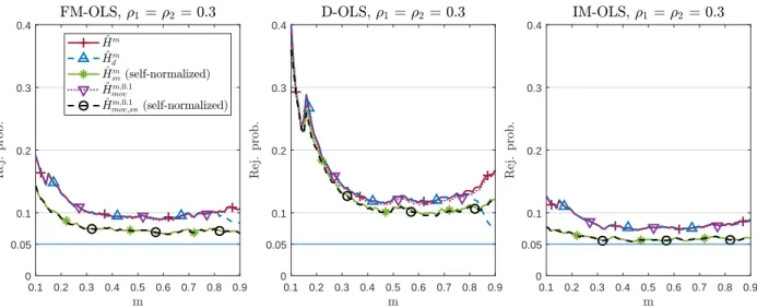
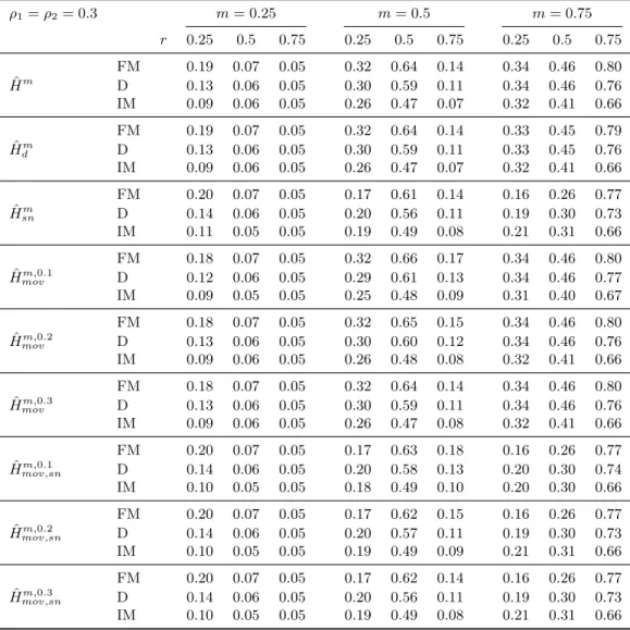
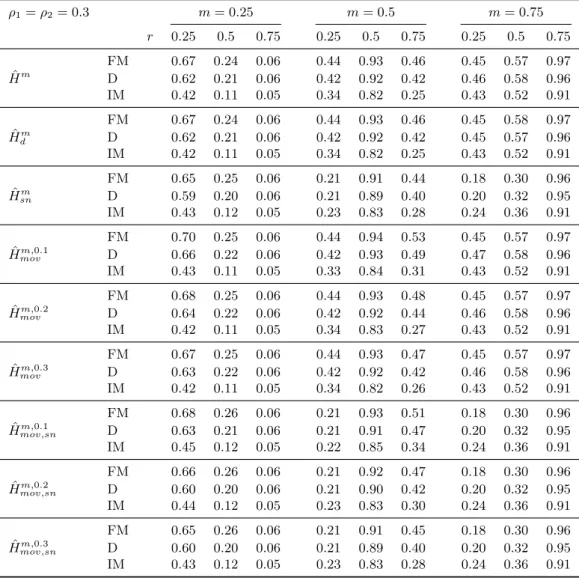
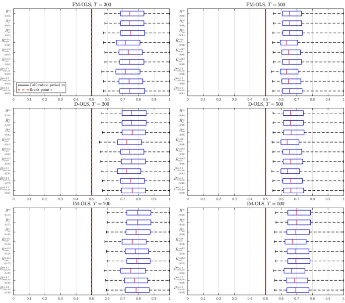
We perform a detailed simulation study of the five considered variants of the monitoring proce- dure in combination with the three mentioned parameter estimation methods. The performance dimensions considered include null rejection probabilities, (empirical) size-corrected power as well as detection delays. It turns out that the combination of self-normalization and a moving window leads almost throughout to the best performance in terms of lowest over-rejections, whilst exhibit- ing very favorable size-corrected power properties and short delays. The choice of the estimator, FM-, D-, or IM-OLS, affects the results in particular for small samples. IM-OLS mostly leads to smaller over-rejections under the null hypothesis than FM-OLS, which in turn outperforms D-OLS.

With respect to size-corrected power IM-OLS is outperformed, as expected, by both FM-OLS and D-OLS. Also, the delays are often a bit smaller for FM-OLS than for IM-OLS. Since the differences are often relatively small, there is no clear choice between IM-OLS and FM-OLS.

We use the developed monitoring tools to assess the stability of environmental Kuznets curves (EKCs) for CO

and SO

emissions for twelve countries using a calibration period 1946–1973 and a monitoring period 1974–2016. The EKC hypothesis postulates an inverted U-shaped relationship between the level of economic development and pollution or emissions.

Brock and Taylor (2005) or Kijima et al. (2010) provide survey discussions of the links between economic activity or growth

4The term EKC refers by analogy to the inverted U-shaped relationship between the level of economic development and the degree of income inequality postulated by Kuznets (1955) in his 1954 presidential address to the American Economic Association. Since the seminal contributions of, e. g. , Grossman and Krueger (1991; 1993; 1995) or Shafik and Bandyopadhyay (1992), the literature – both theoretical as well as empirical – has become voluminous and continues to grow rapidly. Already early survey papers like Yandle et al. (2004) count more than 100 refereed publications on the subject.

and the environment.

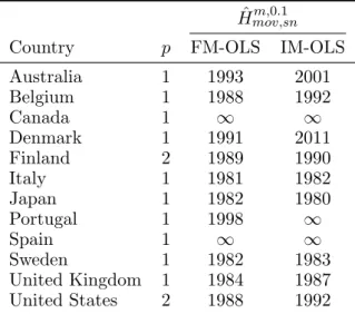
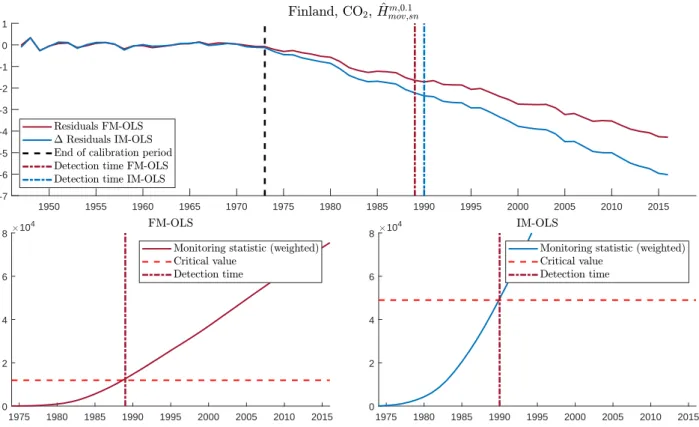
We thus use our monitoring tools to assess whether and if so when the relationship between emissions and economic activity has changed after the first oil price shock, which has led to fundamental changes in economic activity triggered not least by changing energy prices, but also by changes in environmental legislation that has been put in place in the 1970s.

Taking into account that the polynomial functional form should probably be interpreted more as an approximation to an underlying relationship of unknown form rather than as a true relationship, of course, implies a trade-off (at least in-sample) between finding structural breaks and approximation with a higher polynomial degree.

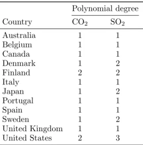
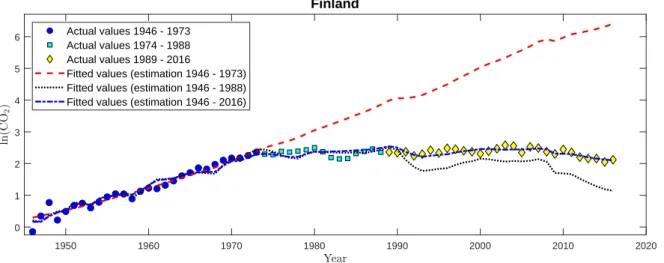
Against this background it may be interesting to use monitoring tools to study whether and at which point in time, the EKC relationship needs to be modelled with more curvature: Over the calibration period 1946–1973 for most countries (as minimum polynomial degree) a cointegrating linear relationship prevails.

This is not a too big surprise, since about until the mid 1970s, economic activity expanded roughly in line with emissions in many countries. Only thereafter and triggered – as mentioned – by price, technical and legislative changes the economic activity and pollution start to be decoupled to a certain extent. From a CPR perspective this could mean either a structural change in the parameters of a relationship of given degree or a change to a relationship with a higher polynomial degree, e. g. , from a linear to a quadratic relationship. For both CO

and SO

emissions for nine of the twelve countries structural breaks are detected. The detected break points are in some cases quite late, which most likely reflects the delays inherent in monitoring procedures. The evidence, when considering also the full sample, is mixed with respect to structural change in the parameters but unchanged polynomial degree or structural change also with respect to the polynomial degree. The monitoring decisions lead to, as a simple empirical cross-check, good results in the following sense: For those country-pollutant combinations where no structural break is detected, using the specification and parameter values from the calibration period leads to good fit also for the full period until 2016, with obviously even better fit when

5The long list of theory contributions presenting specific models that lead to EKC-type behavior under certain assumptions includes Andreoni and Levinson (2001), Arrowet al. (1995), Brock and Taylor (2010), Cropper and Griffiths (1994), Jones and Manuelli (2001), Selden and Song (1995) or Stokey (1998).

6This means that we use our monitoring tools for an ex-post analysis rather than “true” online monitoring.

7This is obvious, since one can achieve perfect fit with a polynomial of degree sample size minus one. There is an ongoing discussion in the EKC literature concerning appropriate functional form and estimation strategies (see, e. g. Bertinelli and Strobl, 2005; Millimet et al., 2003; Schmalenseeet al., 1998). Inverted U-shaped relationships are also considered, e. g. , in the intensity-of-use intensity of use or material Kuznets curve (MKC) literature that investigates the potentially inverted U-shaped relationship between GDP and energy or metals use per unit of GDP (see, e. g. Grabarczyket al., 2018; Guzm´anet al., 2005; Labson and Crompton, 1993; Stuermer, 2018) for which the tools developed in this paper may also be useful.

8A cointegrating linear relationship implies tautologically that CPRs with higher polynomial degrees are also present, albeit with (theoretically) zero coefficients to the higher order powers.

re-estimating the relationship over the full sample.

The paper is organized as follows: Section 2 contains the setting, assumptions, monitoring statis- tics and asymptotic results. Section 3 discusses finite sample simulation results. Section 4 presents the monitoring application to CO

and SO

emissions data. Section 5 briefly summarizes and concludes. Appendix A contains all proofs. In addition, four supplementary appendices are avail- able: Supplementary Appendix B discusses local asymptotic power properties. Supplementary Appendix C contains additional finite sample simulation results and Supplementary Appendix D presents additional empirical results. Supplementary Appendix E includes tables with critical val- ues for the detectors for a broad variety of specifications relevant for EKC-type analysis. MATLAB code – including the critical values for the mentioned variety of specifications – for the monitoring statistics developed in this paper is available upon request.

We use the following notation: Definitional equality is signified by := and ⇒ denotes weak convergence. bxc denotes the integer part of x ∈ R and diag(·) denotes a diagonal matrix. For a vector x ∈ R

we use kxk

= P

i=1

x

and for a matrix M ∈ R

we use kM k = sup

. E (·) denotes the expected value and L is the backward-shift operator, i. e. , L{x

}

= {x

}

. The first-difference operator is denoted with ∆ := 1 − L. We denote the k-dimensional identity matrix with I

. A Brownian motion with covariance matrix specified in the context is denoted by B(r) and W (r) denotes a standard Brownian motion.

2 Theory

2.1 Model, Assumptions and Parameter Estimation

We consider monitoring – using the terminology of Wagner and Hong (2016) – a cointegrating polynomial regression (CPR), i. e. , a regression of the form:

y

=

( D

θ

+ X

θ

+ u

, t = 1, . . . , brT c,

D

θ

+ X

θ

+ u

, t = brT c + 1, . . . , T, (1)

x

= x

+ v

, t = 1, . . . , T, (2)

with x

:= [x

, . . . , x

]

∈ R

and X

:= [x

, x

, . . . , x

]

∈ R

with p = k−1+p

, the deterministic trend function D

∈ R

, the parameter vectors θ

, θ

∈ R

and θ

, θ

∈ R

. Furthermore we define the combined parameter vectors θ := [θ

, θ

]

, θ

:= [θ

, θ

]

∈ R

.

9TheMATLAB code can be straightforwardly modified to other specifications to obtain additional critical values;

under the assumption of full design.

Under the null hypothesis no structural change occurs, that is θ

= θ and {u

}

is an I(0) process, with detailed assumptions specified below, throughout. Under the alternative hypothesis, either some parameters change or the relation turns spurious, i. e. , {u

}

turns into an I(1) process for every θ ∈ R

, or both at a sample fraction brT c that has to be – as discussed in the introduction – larger than bmT c for some 0 < m < 1.

In formal terms:

H

:

( θ

= θ ∀ r ∈ [m, 1) and u

is I (0) for t = 1, . . . , T

H

:



 



 



∃ r ∈ [m, 1) : θ

6= θ or

∃ r ∈ [m, 1) : u

, t = 1, . . . , brT c is I (0) and u

, t = brT c + 1, . . . , T, is I (1).

Remark 1 Note that the regression model given in (1) is a special case of the CPR model con- sidered in Wagner and Hong (2016), since only one of the integrated regressors, w.l.o.g. x

, is allowed to enter the regression model with powers larger than one. Whilst this is, obviously, re- strictive compared to the case where higher order powers of all elements of x

can be present as regressors, this special case covers environmental and material Kuznets curves and similar applica- tions. The mathematical reason for considering this special case is that it allows for – potentially up to a scalar nuisance parameter that can be consistently estimated and scaled out – nuisance parameter free limiting distributions of the considered detectors that can be simulated. In the ter- minology of Vogelsang and Wagner (2014b) a cointegrating polynomial regression needs to exhibit full design to allow for asymptotic standard inference by scaling out a scalar long-run variance.

This is the case for EKC-type relationships with only one integrated regressor present with powers larger than one, but also for some other economically relevant more general cases of CPRs, e. g. , Translog functions (see, e. g. Christensen et al., 1971). Given our focus on EKCs we abstain from formulating the results here in the most general form; the required extensions are straightforward.

For even more general specifications that do not exhibit full design, a sub-sampling approach may be considered relying upon similar arguments as discussed in Wagner and Hong (2016, Proposition 6).

The performance of sub-sampling based procedures, however, suffers particularly from short sample periods; as also illustrated by the simulations reported in Wagner and Hong (2016). Consequently, a sub-sampling based approach cannot be expected to perform well in a monitoring context.

10Effectively,{ut}t∈Zbeing an I(0) process in this paper means that it satisfies Assumption 2. An I(1) process is a process that does not fulfill Assumption 2, but where the first difference does.

The results developed below rest upon the following assumptions:

Assumption 1 There exists a sequence of q ×q scaling matrices G

(T ) and a q-dimensional vector of functions D(z), with R

0

D(z)D(z)

ds < ∞ for 0 ≤ s ≤ 1, such that for 0 ≤ s ≤ 1 it holds that:

T

lim

√

T G

(T )D

= D(s). (3)

If, e. g. , D

:= (1, t, t

, . . . , t

)

, then G

(T ) := diag(T

, T

, T

, . . . , T

) and D(z) = (1, z, z

, . . . , z

)

. In relation to the integrated regressors and the powers we need a scaling matrix G

(T ) := diag(T × I

, T

, . . . , T

) later.

Assumption 2 The process {η

}

:= {[u

, v

]

}

is generated under the null hypothesis as:

η

= C(L)ξ

=

∞

X

j=0

C

ξ

, t ∈ Z, (4)

with C

∈ R

, j = 0, 1, . . . , and the conditions:

det(C(1)) 6= 0,

∞

X

j=0

jkC

k < ∞ and kC

k < ∞. (5) Furthermore, we assume that the process {ξ

}

is a strictly stationary and ergodic martingale difference sequence with natural filtration F

= σ({ξ

}

), E(ξ

ξ

|F

) = Σ

> 0 with in addition sup

E (kξ

k

|F

) < ∞ a.s. for some a > 4.

The assumptions on the deterministic components, the regressors and error terms are similar to the assumptions used in Wagner and Hong (2016) and, more implicitly, in Wagner and Wied (2017). In particular Assumption 2 is sufficient for a functional central limit theorem to hold for {η

}

:

√ 1 T

bsTc

X

t=1

η

⇒ B (s) =

B

(s) B

(s)

= Ω

W (s), 0 ≤ s ≤ 1, (6)

with the positive definite long-run covariance matrix Ω := P

j=−∞

E (η

η

) and W (s) := [W

(s), W

(s)

]

a (k + 1)-dimensional vector of standard Brownian motions. We also define the half long-run co- variance matrix ∆ := P

j=0

E (η

η

). The matrices Ω and ∆ are partitioned according to the partitioning of B(s), i. e. ,

Ω =

Ω

Ω

Ω

Ω

, ∆ =

∆

∆

∆

∆

. (7)

Using, e. g. , the Cholesky decomposition of Ω yields:

Ω

=

"

ω

λ

0 Ω

#

, (8)

where ω

:= Ω

− Ω

Ω

Ω

and λ

:= Ω

(Ω

)

. The conditional long-run variance ω

is a key quantity that needs to be estimated for all but the two self-normalized detectors.

Where needed, consistent long-run covariance estimation is performed non-parametrically, re- quiring the choice of both a kernel function and a bandwidth parameter. The inputs in the non- parametric estimation are the OLS residuals from estimating (1) over the calibration period and the first difference of x

over the same period. For consistent long-run covariance estimation it suffices to assume (following, e. g. , Jansson, 2002):

Assumption 3 The kernel function k(·) satisfies:

(i) k(0) = 1, k(·) is continuous at 0 and k(0) := sup ¯

|k(x)| < ∞, (ii) R

0

¯ k(x)dx < ∞, where k(x) = sup ¯

|k(y)|.

Assumption 4 The bandwidth parameter M

⊆ (0, ∞) satisfies lim

(M

+ T

M

) = 0.

All our monitoring statistics discussed in the following subsection are based on consistent pa- rameter estimators that are required to lead to limiting distributions that are nuisance parameter free up to a scalar parameter, the conditional long-run variance ω

, that can (asymptotically) be scaled out, either by scaling by a consistent estimator, which we refer to later as standardized, or by self-normalization.

As indicated, estimation takes place on the calibration sample t = 1, . . . , bmT c for some 0 < m <

1 that is known to be generated under the null hypothesis. This approach to monitoring, based on parameter estimation on a calibration sample known to be – or at least assumed to be – free of structural change has been popularized in the econometrics community by the seminal work of Chu et al. (1996).

The cointegration literature provides a variety of modified ordinary least squares estimators of θ

with the required asymptotic properties, see, e. g. , Wagner (2018) for a survey. All these estimators

commence from the fact that the OLS estimator of θ is consistent with – in case of regressor

endogeneity and error serial correlation – a limiting distribution that is contaminated by second

order bias terms. These second order bias terms are removed, one way or another, by the various modifications of OLS. In this paper we consider three modified OLS estimators: Fully Modified OLS (FM-OLS), Dynamic OLS (D-OLS) and Integrated Modified OLS (IM-OLS). These three estimators have originally been developed for cointegrating linear regressions: FM-OLS in Phillips and Hansen (1990), D-OLS in Saikkonen (1991), Phillips and Loretan (1991) or Stock and Watson (1993) and IM-OLS in Vogelsang and Wagner (2014a). The extensions to the CPR setting are discussed for FM-OLS in Wagner and Hong (2016), for D-OLS in Choi and Saikkonen (2010) and for IM-OLS in Vogelsang and Wagner (2014b).

Our brief discussion of the three estimators first necessitates the definition of a few more quan- tities, i. e. , Z

:= [D

, X

]

and y

:= y

− ∆x

Ω ˆ

Ω ˆ

, with the second subscript m indicating that estimation of the long-run covariances is – as mentioned – also based on the calibration sample t = 1, . . . , bmT c. Furthermore, define:

A

:=





0

bmT c ∆ ˆ

M



 , M

:= ˆ ∆

ku,m







2 P

x

.. . p

P

t=1

x





 , (9) with ˆ ∆

:= ˆ ∆

Ω ˆ

∆ ˆ

and ˆ ∆

:= ˆ ∆

Ω ˆ

∆ ˆ

.

Long-run covariance estimation uses the OLS residuals of (1) from estimation over the calibration period t = 1, . . . , bmT c in conjunction with the first differences of the integrated regressors, i.e., ˆ

η

:= [ˆ u

, v

]

, with ˆ u

denoting the OLS residuals here:

∆ ˆ

:= 1 bmT c

bmTc−1

X

h=0

k h

M

X

t=1

ˆ

η

η ˆ

, (10)

Σ ˆ

:= 1 bmT c

bmTc

X

t=1

ˆ

η

η ˆ

, (11)

Ω ˆ

:= ˆ ∆

+ ˆ ∆

− Σ ˆ

. (12)

In both the finite sample simulations as well as the application we use for long-run covariance estimation, in line with Assumptions 3 and 4, the Bartlett kernel with bandwidth chosen according to Newey and West (1994).

11To be precise, Choi and Saikkonen (2010) propose an extension of the dynamic regression approach, adding leads and lags of the first differences of the integrated regressors, to a more general setting than CPRs. Given that the CPR model is linear in parameters, D-OLS can be extended relatively straightforwardly, without the need to resort to modified nonlinear least squares type estimators. Vogelsang and Wagner (2014b) consider an extension of IM-OLS to general multivariate polynomials allowing also for arbitrary cross-products of powers of integrated regressors. Stypka and Wagner (2020) extend the FM-OLS estimation principle to this more general polynomial-type setting.

With all required quantities defined, the FM-OLS estimator computed over the calibration sample is given by:

θ ˆ

:=





bmTc

X

t=1

Z

Z





−1





bmTc

X

t=1

Z

y

− A



 . (13) While FM-OLS is based on a two-part nonparametric transformation to remove endogeneity and serial correlation related bias terms from the limiting distribution of the OLS estimator, D- OLS is based on a more “classical projection and orthogonalization” argument by performing OLS estimation in an augmented version of the CPR regression (1), with leads and lags of the first differences of x

added as regressors to “clean the limiting distribution”. The D-OLS regression – estimated by OLS over the calibration sample – is given by:

y

= Z

θ +

d2

X

j=−d1

∆x

Θ

+ u

, (14)

with the number of leads (d

) and lags (d

) chosen to ensure consistent parameter estimation of θ with a limiting distribution that is – up to a scalar – nuisance parameter free. In general this requires that d

, d

→ ∞ at suitable rates. More specifically, in our finite sample simulations and the application, we choose leads and lags using the AIC-type criterion of Choi and Kurozumi (2012). The resultant OLS estimators of θ and ˆ Θ

from (14) estimated over the calibration sample are referred to as ˆ θ

and ˆ Θ

, respectively.

The third estimation principle addresses endogeneity correction by partial summation. Define for a sequence z

, t = 1, . . . , T the partial summed variable by S

:= P

j=1

z

, t = 1, . . . , T . Then the IM-OLS regression – estimated by OLS over the calibration sample – is given by:

S

= S

θ + x

ϕ + S

. (15) The OLS estimators of θ and ϕ from (15) estimated over the calibration sample are referred to as ˆ θ

and ˆ ϕ

, respectively. Note that endogeneity correction in the IM-OLS estimator does not require any leads-lags or kernel-bandwidth choices, as it suffices to simply add the original integrated regressor vector x

to the partial summed regression.

The key input for the monitoring statistics discussed in the following subsection are the resid-

ual (processes) obtained with these three estimators. In particular, the asymptotic null behav-

ior of the residual (partial sum) processes is the key ingredient to derive asymptotic properties

of any of our variance-ratio type monitoring statistics. This result is formalized in the follow- ing lemma, whose formulation requires to define some additional (asymptotic) quantities first, i. e. , W

(s) := [W

(s), W

(s), . . . , W

(s), W

k

(s), . . . , W

(s)]

, J (s) := [D(s)

, W

(s)

]

, f (s) :=

[ R

0

D(z)

dz, R

0

W

(z)

dz, W

(s)

]

and F (s) := R

0

f(z)dz.

Lemma 1 Let the data be generated according to (1) and (2) with Assumptions 1 and 2 in place.

Furthermore, let long-run covariance estimation be performed under Assumptions 3 and 4 and let lead-lag choices be made as discussed in Choi and Kurozumi (2012).

Based on estimation over the calibration period t = 1, . . . , bmT c – with the estimators θ ˆ

, θ ˆ

and θ ˆ

as discussed before – denote the FM-OLS residuals by:

ˆ

u

:= y

− Z

θ ˆ

, (16) the D-OLS residuals by:

ˆ

u

:= y

− Z

θ ˆ

−

d2

X

j=−d1

∆x

Θ ˆ

(17)

and the IM-OLS residuals by:

S ˆ

:= S

− S

θ ˆ

− x

ϕ ˆ

. (18)

For T → ∞ it holds under the null hypothesis for m ≤ s ≤ 1 that:

√ 1 T

S ˆ

:= 1

√ T

bsTc

X

t=2

ˆ

u

⇒ ω

W

(s) − Z

0

J (z)

dz Z

0

J (z)J (z)

dz

Z

J(z)dW

(z)

!

=: ω

W f

(s) (19)

√ 1 T

S ˆ

:= 1

√ T

min{bsTc,T−d1}

X

t=d2+2

ˆ

u

⇒ ω

W f

(s) (20)

√ 1 T

S ˆ

:= 1

√ T

bsTc

X

t=2

∆ ˆ S

⇒ ω

W

(s) − f (s)

Z

0

f(z)f(z)

dz

Z

[F (m) − F (z)]dW

(z)

!

=: ω

P e

(s). (21)

12For the asymptotic results the lower bounds of the summations could all be set equal tot= 1. We, however, start the sums with the first residual actually available for computations, at the expense of potentially making matters appear overly complicated, at least in terms of notation, but replicable for implementation by the reader.

The lemma shows that indeed all three partial sum processes of the residuals converge to processes that are (i) functionals of standard Brownian motions, W

(r) and W

(r), and (ii) proportional to ω

, a scalar nuisance parameter that can be consistently estimated and hence scaled out from the limit processes or that can be eliminated by self-normalization. The limiting null distributions of test statistics based on the (normalized) limit processes consequently can be obtained by simulating the corresponding functionals of standard Brownian motions. Note that the FM-OLS and D-OLS residual partial sum processes converge to the same limiting process, which is a consequence of these two estimators having identical limiting distributions.

2.2 The Monitoring Statistics

Similarly to Wagner and Wied (2017) the starting point of our monitoring statistics is to combine the approach of Chu et al. (1996) with variance-ratio statistics that diverge under the alternative.

More specifically, the underlying variance-ratio (full sample) statistic motivating the construction of our monitoring statistics is the Kwiatkowski et al. (1992) stationarity test, respectively the related Shin (1994) cointegration test.

Using our notation, the (full sample) Shin-statistic is given by:

T

:= 1 ˆ ω



 1 T

T

X

t=1

√ 1 T

t

X

i=1

ˆ u

!



 (22)

= 1

ˆ ω

1 T

T

X

t=1

1

√ T

S ˆ

!

,

with ˆ u

denoting the residuals from (full sample) estimation with, e. g. , FM-OLS or D-OLS. In case that IM-OLS is used for estimation, the resultant residuals are already partial summed quantities, i. e. , one immediately obtains (by construction) quantities to insert into the expression in the second line of (22). The test statistic given above converges under the null hypothesis to a functional of standard Brownian motions, which is as expected when considering (22), where convergence to the squared integral of a standard Brownian motion follows immediately from our assumptions if instead of ˆ u

the errors u

were used (and scaling would take place by a consistent estimator of ω

). Using ˆ u

instead of u

leads to a similar result, but with a different (specification dependent) functional of standard Brownian motions after scaling out ω

rather than ω

. To be precise, when

13For completeness note that the Shin (1994) test has been considered in the CPR setting in Wagner and Hong (2016). In principle, of course, also other variance-ratio type statistics for the null hypothesis of stationarity – or cointegration – could serve as building blocks, e. g. , the test statistic of Busetti and Taylor (2004) or Kim (2000) more or less directly leads, when extended and considered for monitoring, to a self-normalized detector similar to Hˆ_sn^m.

using FM-OLS or D-OLS for parameter estimation the limiting null distribution will be a function of W f

(r). When using IM-OLS for parameter estimation the limiting null distribution will be a function of P e

(r), see Proposition 1 below.

The above test statistic (22) can be easily seen to diverge under the alternative hypothesis of a structural break occurring after the calibration period. Consider, e. g. , the FM-OLS residuals (with the argument entirely analogous for all estimators) using our already established notation:

ˆ

u

:= y

− Z

θ ˆ

(23)

= u

− v

Ω ˆ

Ω ˆ

− D

(ˆ θ

− θ

) − X

(ˆ θ

− θ

)

√ 1 T

bsTc

X

t=2

ˆ

u

= 1

√ T

bsTc

X

t=2

u

− 1

√ T

bsTc

X

t=2

v

Ω ˆ

Ω ˆ

− 1

√ T

bsTc

X

t=2

D

(ˆ θ

− θ

) (24)

− 1

√ T

bsTc

X

t=2

X

(ˆ θ

− θ

)

Now, suppose that at some time point brT c > bmT c a structural change occurs. If, e. g. , {u

}

turns from being I(0) to I(1), then the first term in (24) diverges for s > r. Similarly, the third or fourth term (or both) diverge in case of change in the parameter vector, i. e. , when θ

6= θ, as of course ˆ θ

→ θ, because of parameter estimation on the calibration sample.

We consider for each of the three considered estimators – neglecting for notational brevity the dependence of the residuals and thus the test statistics on the estimation method – five monitoring statistics:

H ˆ

(s) := 1 ˆ ω



 1 T

bsTc

X

i=bmTc+1

1

√ T

S ˆ



 (25)

H ˆ

(s) := 1 ˆ ω



 1 T

bsTc

X

i=bmTc+1

1

√ T S ˆ

− 1 T

bmTc

X

i=1

1

√ T S ˆ



 (26)

H ˆ

(s) :=

P

S ˆ

P

S ˆ

(27) H ˆ

(s) := 1

ˆ ω



 1 T

bsTc

X

i=max{1,bsTc−bnTc+1}

1

√ T

S ˆ



 (28)

H ˆ

(s) :=

P

i=max{1,bsTc−bnTc+1}

S ˆ

P

S ˆ

(29)

The monitoring statistic ˆ H

(s) given in (25) is of the same form as the monitoring statistic used in Wagner and Wied (2017) considered here in the CPR context. The monitoring statistic ˆ H

(s) given in (26) – with a term calculated only over the calibration sample subtracted – is of a similar form as used in Chu et al. (1996). The third variant ˆ H

(s) given in (27) is a self-normalized statistic, for which under the null hypothesis both the numerator and denominator converge (appropriately scaled) to functionals of standard Brownian motions proportional to ω

, which is hence scaled out in the ratio. Long-run covariance estimation is known to be a notoriously problematic aspect in unit root and cointegration analysis and therefore test statistics that do not require this step may exhibit better performance. The fourth considered variant is a moving window statistic ˆ H

given in (28) with n denoting the moving window (sample fraction or) length. The key difference between the moving window detector and the expanding window detectors is that ˆ H

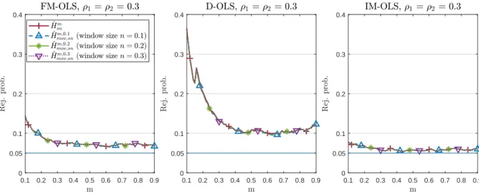
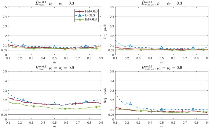
is based on a constant number of residual partial sums for all values of s. This construction increases, under the alternative hypothesis, the impact of post-break residuals on the test statistic, which is ex ante expected to lead to faster detection of structural breaks. The performance of the fourth variant will depend on the length of the moving window, to be chosen in applications. Finally, the fifth monitoring statistic H

given in (29) combines self-normalization and moving window estimation, with the performance as for the fourth variant expected to depend upon the moving window length.

The following proposition summarizes the asymptotic behavior of the monitoring statistics under the null hypothesis.

Proposition 1 Let the data be generated according to (1) and (2) with Assumptions 1 and 2 in place. Furthermore, let long-run covariance estimation be performed under Assumptions 3 and 4 and let lead-lag choices be made as discussed in Choi and Kurozumi (2012).

In case parameter estimation is performed with FM-OLS or D-OLS the limiting process Q e

(s) below equals W f

(s) and in case parameter estimation is performed by IM-OLS it equals P e

(s).

The defined monitoring statistics converge under the null hypothesis for T → ∞, in particular it

14To be precise, only when using ˆHsn^m(s) or ˆHmov,sn^m,n (s) in conjunction with D-OLS or IM-OLS no long-run co- variance estimators are required, whereas estimated long-run covariances are required for FM-OLS estimation. For D-OLS still lead-lag length choices have to be made and only when using ˆHsn^m(s) or ˆHmov,sn^m,n (s) in conjunction with the IM-OLS estimator no kernel/bandwidth or lead-lag choices have to be made. In this case, the only choice to still be made when using ˆHsn^m(s) is the length of the calibration sample, a choice required throughout. In case of Hˆ_mov,sn^m,n (s) both the calibration sample lengthmand the moving window lengthnhave to be chosen.

holds that:

H ˆ

(s) ⇒ Z

m

Q e

(z)dz =: H

( Q e

, s) (30) H ˆ

(s) ⇒

Z

Q e

(z)dz − Z

0

Q e

(z)dz =: H

( Q e

, s) (31) H ˆ

(s) ⇒

R

m

Q e

(z)dz R

0

Q e

(z)dz =: H

( Q e

, s) (32) H ˆ

(s) ⇒

Z

max{0,s−n}

Q e

(z)dz =: H

( Q e

, s) (33) H ˆ

(s) ⇒

R

max{0,s−n}

Q e

(z)dz R

0

Q e

(z)dz =: H

( Q e

, s) (34) It is widely-used practice in monitoring to base the decision not on monitoring statistics as just defined, but on monitoring statistics divided by a weighting function, g(s) say. For chosen weighting function g(s) – with 0 < g(s) < ∞ – the null hypothesis is rejected, if the weighted monitoring statistic

H(s)ˆ g(s)

is larger than a critical value c for the first time. We denote this point in time as detection time τ

, i.e.:

τ

:= min

s:bmTc+1≤bsTc≤T

(

H(s) ˆ g(s)

> c )

, (35)

with ˆ H(s) short-hand notation for any of the considered detectors. In case no structural change is detected, i. e. ,

Hˆ(s) g(s)

≤ c for all m ≤ s ≤ 1, we set τ

= ∞. A finite value of τ

not only indicates a structural break but also contains information about the location of the potential break point.

Weighting function and critical value have to be chosen so that under the null hypothesis it holds that:

T

lim

P (τ

< ∞) = lim

T→∞

P min

s:[mT]+1≤[sT]≤T

(

H(s) ˆ g(s)

> c )

< ∞

!

= lim

T→∞

P sup

s:[mT]+1≤[sT]≤T

H(s) ˆ g(s)

> c

!

(36)

= P

sup

m≤s≤1

H(s) g(s)

> c

= α,

with α denoting the chosen significance level, and H(s) short-hand notation for the limit corre-

sponding to the considered monitoring statistic. Considering only positive and bounded weighting

functions, see also Aue et al. (2012, Assumption 3.6), allows to derive the required result given above

based on the developed asymptotic null behavior of the monitoring statistics and the continuous

mapping theorem.

Proposition 2 Let the data be generated according to (1) and (2) with Assumptions 1 and 2 in place. Furthermore, let long-run covariance estimation be performed under Assumptions 3 and 4 and let lead-lag choices be made as discussed in Choi and Kurozumi (2012). In addition assume that the weighting function g(s) is continuous and bounded. Then there exist critical values c = c(α, g, m, n) such that for any 0 < α < 1 it holds that:

T

lim

P

τ

( ˆ H(s), g(s), c) < ∞

= α (37)

Clearly, the choice of a weighting function g(s) impacts the performance of monitoring procedures and has to combine two opposing goals: (i) small size distortions under the null hypothesis and (ii) small delays under the alternative hypothesis, that is, detection of a break as soon as possible after the break. The discussion in Chu et al. (1996, Section 3) makes clear that it is in general, even in more standard regression models, impossible to derive analytically tractable optimal weighting functions (from a certain class of functions), e. g. , with respect to minimal expected delay.

Given the lack of analytical results concerning optimal choices of weighting functions we have performed a large number of preliminary simulations using a range of candidate weighting func- tions.

The starting point of these considerations is Wagner and Wied (2017), who choose the weighting function in relation to the expected value of the monitoring statistics, resulting in g(s) = s

in case D

= 1 (intercept only) and g(s) = s

in case D

= [1, t]

(intercept and linear trend). In case of a linear trend we have in addition experimented with g(s) ∈ {1, s

, s

, s

, √

m(1 +

),

}, with the last two functions inspired by Horv´ ath et al. (2004).

It turns out that no weighting, i. e. , g(s) = 1 does not lead to favorable performance compared to g(s) = s

or s

. The function s

is chosen by “extrapolation” of the fact that s

works better than s

= 1. The idea of the third and fourth functions is – merely the result of some experimentation and heuristics – to make the detector more sensitive by increasing the value of the statistic whilst at the same leaving the critical values effectively unchanged. The effects are

15Aueet al.(2009) derive the limiting distributions of the delay time for a one-time parameter change in a linear regression model with stationary errors for a simple class of weighting functions depending only upon a single (tuning) parameter. The situation is much more involved in our context and any result concerning asymptotic distributions of delay times will depend upon intricate crossing-probability calculations involving complicated functions of Brownian motions. Results in this direction therefore appear to be very hard to obtain, for us at least.

16We have performed the type of simulations reported in Section 3 investigating the performance with respect to null rejection probabilities, size corrected power and detection times for all weighing functions discussed here. The simulations in Section 3 report the results based on the overall best performing weighting function,s³(intercept only) ands⁵ (intercept and linear trend).

17In the intercept only specification the set of functions considered is given by{1, s⁶, s^3(0.5+m), s^3(0.85+m)2,√ m(1 +

s−m

m ),^√s_m ^s−m_s 1/2

}. The observations are similar for both specifications of the deterministic component.

to a certain extent as expected, without, however, leading to overall better performance. Taking s

= (s

)

or s

= (s

)

as weighting functions does indeed lead, e. g. , to earlier detection times, however, often also to detections in cases when there is no structural change, i. e. , these functions lead to larger over-rejections under the null hypothesis. The two functions s

, s

, where we have also experimented with other powers and values, try to strike a balance between earlier rejections and size distortions. Altogether, however, the simple functions s

and s

perform most stably over a variety of configurations, in terms of comparably low size distortions under the null as first priority and short delays in the detection times.

Finally, the two functions inspired by Horv´ ath et al. (2004), where we have also experimented with different powers, lead to essentially the same null rejection probabilities and size corrected power as, e. g. , s

or s

, but lead to partly substantially bigger delays than the other weighting functions. Therefore, we stick to the weighting functions already used also in Wagner and Wied (2017), i. e. , the end point of the considerations is the starting point. As mentioned, it remains an open challenge to make progress on finding optimal weighting functions for the monitoring problem and detectors considered in this paper, or more generally when monitoring cointegrating relationships.

It remains to characterize the asymptotic behavior of the proposed monitoring procedures under the relevant alternatives in our setting: First, the error process {u

}

changes its behavior from I(0) to I(1), i. e. , it changes to being an integrated process and second, there are breaks in (some of) the parameter values. For both cases we consider the asymptotic behavior against fixed and local alternatives, with the local alternatives having to be specified, as always, in line with the convergence rates of parameter estimation.

Proposition 3 Let the data be generated for t = 1, . . . , brT c according to (1) and (2) with As- sumptions 1 and 2 in place. Furthermore, let long-run covariance estimation be performed under Assumptions 3 and 4 and let lead-lag choices be made as discussed in Choi and Kurozumi (2012). In addition assume that the weighting function g(s) is continuous, positive and bounded. Furthermore, H(s) ˆ denotes again any of the considered monitoring statistics.

(a) Let

(i) {u

}

be an I (1) process from brT c + 1 onwards, or

18More specifically, the simpler functions lead to the lowest over-rejections almost throughout, the “race” in terms of size-corrected power is relatively even, and in some cases the more complicated weighting functions, in particular s^3(0.85+m)2 ors^5(0.85+m)2 lead to slightly smaller delays.