The Asymptotic Validity of "Standard" Fully Modified OLS Estimation and Inference in Cointegrating Polynomial Regressions

IHS Economics Series Working Paper 333

October 2017

The Asymptotic Validity of

"Standard" Fully Modified OLS Estimation and Inference in Cointegrating Polynomial Regressions

Oliver Stypka

Martin Wagner

Peter Grabarczyk

Rafael Kawka

Impressum Author(s):

Oliver Stypka, Martin Wagner, Peter Grabarczyk, Rafael Kawka Title:

The Asymptotic Validity of "Standard" Fully Modified OLS Estimation and Inference in Cointegrating Polynomial Regressions

ISSN: 1605-7996

2017 Institut für Höhere Studien - Institute for Advanced Studies (IHS) Josefstädter Straße 39, A-1080 Wien

E-Mail: o ce@ihs.ac.atffi Web: ww w .ihs.ac. a t

All IHS Working Papers are available online: http://irihs. ihs. ac.at/view/ihs_series/

The Asymptotic Validity of “Standard”

Fully Modified OLS Estimation and Inference in Cointegrating Polynomial

Regressions

Oliver Stypka

, Martin Wagner

, Peter Grabarczyk

and Rafael Kawka

1Faculty of Statistics, Technical University Dortmund

2Institute for Advanced Studies, Vienna

3Bank of Slovenia, Ljubljana

Proposed running head:

“Standard” FM-OLS in CPRs

Corresponding author:

Martin Wagner Faculty of Statistics Technical University Dortmund

Vogelpothsweg 87 44227 Dortmund, Germany

Tel: +49 231 755 3174

Email: mwagner@statistik.tu-dortmund.de

Abstract

The paper considers estimation and inference in cointegrating polynomial regres- sions, i. e., regressions that include deterministic variables, integrated processes and their powers as explanatory variables. The stationary errors are allowed to be se- rially correlated and the regressors are allowed to be endogenous. The main result shows that estimating such relationships using the Phillips and Hansen (1990) fully modified OLS approach developed for linear cointegrating relationships by incor- rectly considering all integrated regressors and their powers as integrated regressors leads to the same limiting distribution as the Wagner and Hong (2016) fully modified type estimator developed for cointegrating polynomial regressions. A key ingredi- ent for the main result are novel limit results for kernel weighted sums of properly scaled nonstationary processes involving scaled powers of integrated processes. Even though the simulation results indicate performance advantages of the Wagner and Hong (2016) estimator that are partly present even in large samples, the results of the paper drastically enlarge the useability of the Phillips and Hansen (1990) esti- mator as implemented in many software packages.

JEL Classification: C13, C32

Keywords: Cointegrating Polynomial Regression, Cointegration Test, Environmen- tal Kuznets Curve, Fully Modified OLS Estimation, Integrated Process, Nonlinearity

1. Introduction

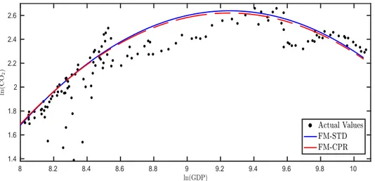
One motivation to consider cointegrating polynomial regressions (CPRs), using the ter- minology of Wagner and Hong (2016), is the environmental Kuznets curve (EKC) lit- erature that investigates a potentially inverted U-shaped relationship between measures of economic development (typically proxied by GDP per capita) and pollution. This literature grows at rapid pace since the seminal work of Grossman and Krueger (1995).¹ Early survey papers, like Yandle et al. (2004), count more than 100 refereed publica- tions already more than a decade ago. As an example of the relationship considered in this literature consider the scatterplot between the logarithm of GDP per capita and the logarithm of CO₂ emissions per capita in Belgium over the period 1870–2009 in Figure 1.

The estimation results also shown in this figure are obtained from estimating the rela- tionship:

ln(CO₂)_t=c+δt+β₁ln(GDP)_t+β₂ln(GDP)²_t +u_t, (1) where the logarithm of Belgian GDP per capita is well-described as an integrated pro- cess of order one, compare Wagner (2015). With a stationary error term, the above relationship is a CPR relationship. An integrated process and its square cannot both be integrated processes of order one (see, e. g., Wagner, 2012) and obviously there is an exact deterministic relationship between the logarithm of GDP per capita and its square. These basic observations lead Wagner and Hong (2016) to a reconsideration and extension of the fully modified OLS (FM-OLS) estimator of Phillips and Hansen (1990) from the linear cointegration setting to the CPR setting.² The corresponding

1The term EKC refers by analogy to the inverted U-shaped relationship between the level of economic development and the degree of income inequality postulated by Simon Kuznets (1955) in his 1954 presidential address to the American Economic Association.

Inverted U-shaped relationships are also prominent in other areas, including the so-called intensity- of-use literature investigating the relationship between energy or material intensity and GDP per capita, see, e. g., Malenbaum (1978) or Labson and Crompton (1993).

2As discussed in Wagner and Hong (2016), similar results are or could also be obtained under alternative assumptions that partly need to be augmented to accommodate powers of integrated regressors, see, e. g., Chan and Wang (2015), Changet al.(2001), de Jong (2002), Ibragimov and Phillips (2008) or Lianget al.(2016). A key difference between the results here and those of, e. g., Changet al.(2001) is that{ut}t∈Z is allowed to be serially correlated, in an MDS setting in Wagner and Hong (2016) and in a linear process setting in this paper. Wang (2015) is an excellent monograph on asymptotic theory for nonlinear cointegration in a regression framework.

8 8.2 8.4 8.6 8.8 9 9.2 9.4 9.6 9.8 10 1.4

1.6 1.8 2 2.2 2.4 2.6

Figure 1: Estimated EKC for CO₂ emissions for Belgium over the period 1870–2009;

variables in logarithms of per capita quantities. The curves result from inserting 140 equidistantly spaced observations from the sample range of ln(GDP), with trend values given by t = 1, . . . ,140, in the estimated relationship (1). The solid line corresponds to the FM-STD coefficient estimates and the dashed line to the FM-CPR coefficient estimates.

estimation results, referred to as FM-CPR in this paper are displayed as the dashed line in Figure 1.

The solid line also displayed in Figure 1 corresponds to how cointegration methods are routinely used in the EKC literature: The estimates are derived from treating (1) as if it were a linear cointegrating relationship with two integrated regressors, estimated using, e. g., the FM-OLS estimator of Phillips and Hansen (1990). Both, log GDP per capita and its square are thereby considered as integrated processes of order one that are furthermore assumed to be not cointegrated. This estimator is referred to as FM-STD estimator in this paper.

Given the differences between a linear cointegration relationship and a cointegrating polynomial relationship it appears to be misguided to use the FM-STD estimator in a cointegrating polynomial regression. However, the figure displays that the results are very similar, an observation also made with data for 19 countries in Wagner (2015). This paper provides an asymptotic explanation for such similar findings: The two estimators, FM-CPR and FM-STD, have the same asymptotic distribution in the CPR case. This result holds true for the general CPR case considered in Wagner and Hong (2016), with multiple integrated regressors, arbitrary polynomial powers and general deterministic components. A practical implication of this result is that one can use standard soft-

ware package implementations of FM-OLS of Phillips and Hansen (1990) for estimation and inference in cointegrating polynomial relationships by “formally” (for the software) considering all integrated regressors and their powers as integrated regressors.³ The only restriction for the result to hold is that the estimated relationship includes the first powers of all integrated regressors. This restriction is directly related to the following main observation, discussed in detail in Section 2.3: A key step in FM-OLS-type estima- tion is an asymptotic orthogonalization of two Brownian motions to obtain a zero mean Gaussian mixture limiting distribution. Given that Brownian motions are by definition Gaussian, achieving independence is equivalent to achieving uncorrelatedness. The latter is obtained by the first-step modification of the dependent variable not only of FM-CPR, but also by the first-step modification of FM-STD, if the first powers of the integrated regressors are all included in the regression. In a sense made precise below, FM-STD thus contains and calculates superfluous quantities in the orthogonalization step (and also in the bias correction step).

The second key ingredient, of independent interest also in other contexts, are weak convergence results for kernel weighted sums (“long-run covariance estimators”) of – properly scaled – processes involving powers of integrated processes. These arise in both transformations that the FM estimation principle is based upon, in the modification of the dependent variable and in the additive bias correction. Turning back to our example equation (1), with full details and all definitions contained in Section 2.3, the dependent variable, logarithm of CO₂ emission per capita, y_t for brevity, is changed to

y_t⁺⁺=yt−[∆xt,∆x²_t] ˆΩ⁻¹_wwΩˆwu (2)

=yt−[∆xt,2xt∆xt−(∆xt)²] ˆΩ⁻¹_wwΩˆwu

withx_t denoting the logarithm of GDP per capita. Usingw_t= [∆x_t,2x_t∆x_t−(∆x_t)²]⁰, the above transformation involves “long-run covariance” estimators involving (in the quadratic case) not only a stationary process, ∆xt, but also xt∆xt. In this paper we derive the weak limits of this type of “long-run covariance” estimators (after proper scaling of the involved quantities). The limits obtained for this type of quantity exhibit exactly the structure that is key for establishing asymptotic equivalence of FM-STD and FM-CPR.

3For notational brevity we focus in the main text on the single integrated regressor case, which facilitates reading and suffices to see all elements required for the results “in action”. In Appendix C we outline the changes and modifications necessary for the multiple integrated regressor case.

The asymptotic equivalence of the estimators implies asymptotic equivalence also of residual based cointegration test like, e. g., the Shin (1994) test. This test has been extended to CPRs in Wagner and Hong (2016) and Wagner (2013), with critical val- ues depending as usual in the cointegration literature upon the specification of the cointegrating polynomial relationship. The EKC literature uses the FM-STD residu- als (which is asymptotically valid), but in conjunction with the original Shin (1994) critical values. This combination results in asymptotically invalid inference, as discussed in Section 2.4.

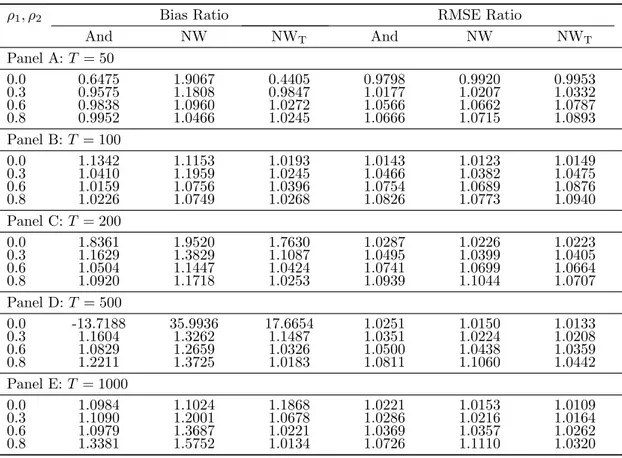
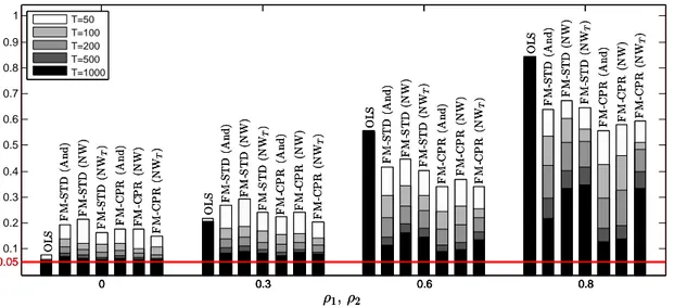
The simulation results indicate that FM-CPR outperforms FM-STD in case of large endogeneity and serial correlation of the errors despite asymptotic equivalence even in large samples like T = 1000. In these cases the calculation of superfluous quantities alluded to above and explained in more detail in Section 2.3 impacts the performance of FM-STD detrimentally. The performance advantages occur in all considered dimensions, estimator bias and RMSE, performance of parameter hypothesis tests, and performance of cointegration tests. In case of data with little or no endogeneity and serial correlation the differences between the estimators more or less vanish for the larger sample sizes considered. Big differences occur for cointegration testing, even when the cointegration test calculated from the FM-STD residuals is used in conjunction with the correct rather than the Shin (1994) critical values.

The paper is organized as follows: In Section 2 we present the setting, the assump- tions and the theoretical results. Section 3 contains a small selection of results from a simulation study assessing the finite sample differences between the two asymptotically equivalent estimators and test statistics based upon them. Section 4 briefly summarizes and concludes. Three appendices follow the main text: Appendix A contains some aux- iliary lemmata, Appendix B contains the proofs of the main results and Appendix C illustrates how to modify the main arguments of the proofs to cover the general, multi- ple integrated regressor case. Supplementary material available upon request contains additional simulation results.

We use the following notation: Definitional equality is signified by :=, equality in distri- bution by=, weak convergence by^d ⇒and convergence in probability by→. We use^P O_P(1) to denote boundedness in probability. Witho_P(1) ando_a.s.(1) we denote convergence to zero in probability and almost surely respectively. The integer part of x ∈ R is given by bxc and a diagonal matrix with entries specified throughout by diag(·). For a vector x= (x_i)_i=1,...,n we denote its Euclidean norm withkxk:= P_n

i=1x²_i1/2

. For a matrix A

the (i, j)-element is denoted withA_(i,j), itsj-th column is labeled byA_(·,j), 0m×ndenotes an (m×n)-matrix with all entries equal to zero andeⁿ_m denotes them-th unit vector in Rⁿ. The Kronecker product is denoted by ⊗. We use Eto denote expectation and L is the backward-shift operator, i. e., L{x_t}_t∈Z={x_t−1}_t∈Z. The first-difference operator is denoted with ∆, i. e., ∆ := 1−L. Brownian motions, with covariance matrices specified in the context, are denoted byB(r). Standard Brownian motion is denoted byW(r).

2. Theory

2.1. Setup and Assumptions

As mentioned in the introduction, it suffices to consider a cointegrating polynomial regression with only one integrated regressor and its powers:⁴

y_t=D⁰_tδ+X_t⁰β+u_t, for t= 1, . . . , T, (3) x_t=xt−1+v_t,

where yt is a scalar process, Dt ∈ R^q is a deterministic component, xt is a scalar I(1) process and X_t := [x_t, x²_t, . . . , x^p_t]⁰ ∈ R^p. Denoting with Z_t := [D⁰_t, X_t⁰]⁰ ∈ R^q+p the stacked regressor vector and withθ:= [δ⁰, β⁰]⁰ ∈R^q+p the parameter vector, equation (3) can be rewritten more compactly as:

y_t=Z_t⁰θ+u_t, fort= 1, . . . , T. (4) Assumption 1. For the deterministic component we assume that there exists a sequence of q×q scaling matrices GD =GD(T) and a q-dimensional vector of c`adl`ag functions D(s), with 0 < Rs

0 D(z)D(z)⁰dz < ∞ for 0 < s ≤ 1, such that for 0 ≤ s ≤ 1 it holds that:

Tlim→∞T^1/2G_DD_bsTc=D(s). (5)

4Clearly, not all consecutive powers ofxt need to be included and in the multiple integrated regressor case the included powers may differ across integrated variables. These changes only complicate “book- keeping”. What is, however, important for asymptotic equivalence is that the integrated variablext

itself is included in the regression, as discussed in detail at the end of Section 2.3. The initial value x0is allowed to be any well-definedO_P(1) random variable.

For the leading case of polynomial time trends, i. e., D_t = [1, t, t², . . . , t^q−1]⁰, clearly G_D = diag(T^−1/2, T^−3/2, T^−5/2, . . . , T^−(q−1/2)) andD(s) = [1, s, s², . . . , s^q−1]⁰.⁵

The precise assumptions concerning the error process and the regressor are as follows:

Assumption 2. The processes {u_t}t∈Z and {∆x_t}t∈Z={v_t}t∈Z are generated as:

u_t=C_u(L)ζ_t=

∞

X

j=0

c_ujζt−j, (6)

∆x_t=v_t=C_v(L)ε_t=

∞

X

j=0

c_vjεt−j, (7)

with P∞

j=0j|c_uj|<∞, P∞

j=0j|c_vj| <∞ and Cv(1)6= 0. Furthermore, we assume that the process {ξ_t⁰}_t∈Z := {[ζ_t, ε_t]⁰}_t∈Z is independently and identically distributed with E(kξ⁰_tk^l) < ∞ for some l > max(8,4/(1−2b)) with 0 < b < 1/3 and positive definite covariance matrix Σ_ξ⁰_ξ⁰.

The above Assumption 2 is stronger than the corresponding assumption in Wagner and Hong (2016). To draw upon some of the results of Kasparis (2008) we replace the mar- tingale difference sequence assumption of Wagner and Hong (2016) with a linear process assumption and the moment assumption of Kasparis (2008).⁶ For univariate {x_t}t∈Z

the assumption C_v(1) 6= 0 excludes stationary {x_t}_t∈Z, and has to be modified in the multivariate case to det(Cv(1))6= 0, i. e., in the multivariate case (e. g. in the discussion in Appendix C) the vector process{x_t}t∈Z is assumed to be non-cointegrated.

For long-run covariance estimation we closely follow Jansson (2002) with respect to our assumptions concerning kernel and bandwidth:

Assumption 3. The kernel functionk(·) satisfies:

1. k(0) = 1, k(·) is continuous at 0 and ¯k(0) := sup_x≥0|k(x)|<∞ 2. R∞

0 ¯k(x)dx <∞, where ¯k(x) = sup_y≥x|k(y)|

5In the EKC literature the deterministic component typically consists of an intercept and a linear trend;

with the latter intended to capture autonomous energy efficiency increases.

6Note that Kasparis (2008, Assumption 1(b), p. 1376) posits the conditionl >min(8,4/(1−2b)). In the proof of his Lemma A1, however, at different places moments of order 4/(1−2b) (p. 1391) and order 8 (p. 1395) are needed. Thus, we believe that the minimum should be replaced by the maximum.

Since we rely upon similar arguments in the proofs of our Lemma 4 we require moments of order max(8,4/(1−2b)).

Assumption 4. The bandwidth parameter M_T → ∞ fulfills M_T = O(T^b), with the same parameterb as in Assumption 2.

The bandwidth Assumption 4 implies limT→∞(M_T⁻¹+T^−1/3MT) = 0, whereas Jansson (2002) assumes lim_T→∞(M_T⁻¹+T^−1/2M_T) = 0, which corresponds toM_T =O(T^b), with 0 < b < 1/2. Thus, we require a tighter upper bound on the bandwidth. This stems from the fact that in the asymptotic analysis of the FM-STD estimator kernel “long-run covariance” estimators involving (properly scaled) powers of integrated processes need to be analyzed. For these quantities we establish weak convergence results under the more restrictive Assumption 4 on the bandwidth. In order to have uniform notation we formally define:

Definition 1. For two sequences {a_t}_t=1,...,T and {b_t}_t=1,...,T we define:⁷

∆ˆab:=

MT

X

h=0

k h

MT

1 T

T−h

X

t=1

atb⁰_t+h, (8)

neglecting the dependence on k(·), M_T and the sample range 1, . . . , T for brevity. Fur- thermore,

Ωˆ_ab:= ˆ∆_ab+ ˆ∆⁰_ab−Σˆ_ab, (9) withΣˆ_ab := _T¹ PT

t=1atb⁰_t.

Based on these quantities we furthermore define ∆ˆ⁺_ab := ˆ∆_ab−∆ˆ_aaΩˆ⁻¹_aaΩˆ_ab and ωˆ_a·b :=

Ωˆ_aa−Ωˆ_abΩˆ⁻¹_bb Ωˆ_ba.

In case that{a_t}_t∈Zand{b_t}_t∈Zare jointly stationary processes with finite half long-run covariance ∆ab :=P∞

h=0E(a0b⁰_h), then under appropriate assumptions ˆ∆abis a consistent estimator of ∆_ab, with a similar result holding for Σ_ab := E(a₀b⁰₀) and a fortiori for Ω_ab:=P∞

h=−∞E(a0b⁰_h).

Remark 1. Note that in our definition of ˆ∆_ab in (8) we use the bandwidth M_T (like, e. g., Phillips, 1995) rather than T−1 (like, e. g., Jansson, 2002) as upper bound of the summation over the index h. For truncated kernels, with k(x) = 0 for |x| > 1, this is of course inconsequential. It can also be shown (based on, e. g., Jansson, 2002) that for “standard” long-run covariance estimation problems, consistency is not affected by

7The standard notation for half long-run covariances is ∆ and therefore we also use this letter. We are confident that no confusion with the first difference operator, also labeled ∆, arises.

the summation index choice, M_T or T −1, for untruncated kernels like the Quadratic Spectral kernel either. In our setting, where the asymptotic behavior of ˆ∆-quantities is analyzed for (properly scaled) nonstationary processes (in Theorem 1 and Corollary 1), the summation bound is important. A key result of this paper, given in Theorem 1 below, hinges upon summation only up to M_T. More specifically, we rely upon the summation bound MT in the proof of Lemma 4, which is related to Kasparis (2008, Lemma A1, p. 1394–1396), where the summation bound M_T is also used (in a slightly different context).

Assumption 2 implies that the process{ξ_t}_t∈Z:={[u_t, vt]⁰}_t∈Zfulfills a functional central limit theorem of the form:

1 T^1/2

brTc

X

t=1

ξ_t⇒B(r) =

"

Bu(r) Bv(r)

#

= Ω^1/2_ξξ W(r), r∈[0,1], (10) with the covariance matrix Ω_ξξ of B(r) given by the long-run covariance matrix of {ξ_t}_t∈Z, i. e.,

Ω_ξξ :=

"

Ωuu Ωuv

Ω_vu Ω_vv

#

=

∞

X

h=−∞

E(ξ₀ξ_h⁰). (11) Later we will also need the corresponding half (or one-sided) long-run covariance matrix

∆_ξξ :=P∞

h=0E(ξ₀ξ_h⁰) partitioned similarly as Ω_ξξ. As is well-known, for FM-type esti- mation, estimates of the half long-run and long-run covariances ∆ and Ω are required.

With (9) holding by definition, we focus below on the estimation of ∆ and Σ. For actual calculations furthermore the unobserved errors u_t are replaced by the OLS residuals ˆu_t from (3), defining ˆξ_t:= [ˆu_t, v_t]⁰.⁸

2.2. Fully Modified OLS Estimation

Wagner and Hong (2016) extend the fully modified OLS (FM-OLS) estimator of Phillips and Hansen (1990) from the linear cointegration to the cointegrating polynomial regres- sion (CPR) case. This estimator, briefly described next, is referred to as FM-CPR in this paper.

8We keep using, e. g., ˆΩξξwhen using the observable ˆutinstead ofutin long-run covariance estimation.

Infeasible estimation involving the unobserved errorsutis labeled with a tilde-symbol, e. g., ˜Ωξξ, see Theorem 1 below.

As in the linear cointegration case, FM-type estimation entails two modifications. The first modification is exactly as in the linear case, with the dependent variabley_treplaced by

y⁺_t :=y_t−∆x_tΩˆ⁻¹_vvΩˆ_vu. (12) This transformation dynamically orthogonalizes the limit partial sum process of the modified errors u⁺_t := ut−vtΩˆ⁻¹_vvΩˆvu, i. e., Bu·v(r) defined below, from the limiting process corresponding to x_t, i. e., B_v(r). In case of Gaussian limits, uncorrelatedness is equivalent to independence, thusBu·v(r) is “automatically” also independent of powers of B_v(r), also occurring in the asymptotic distributions in the CPR case. Consequently, the modification to orthogonalize regressors and errors need not be changed when considering FM-OLS estimation in the CPR setting rather than in the linear cointegration setting;

orthogonalization with respect toB_v(r) suffices.

The second modification, correcting for additive bias terms, depends upon the precise form of the model considered. For specification (3) the bias correction term is given by:

A^∗ := ˆ∆⁺_vu



















0q×1

T 2PT

t=1x_t ... pPT

t=1x^p−1_t



















, (13)

with ˆ∆⁺_vu := ˆ∆_vu−∆ˆ_vvΩˆ⁻¹_vvΩˆ_vu. Defining y⁺ := [y⁺₁, . . . , y_T⁺]⁰ and Z := [Z₁, . . . , Z_T]⁰, leads to the FM-CPR estimator ofθ given by:

θˆ⁺:= (Z⁰Z)⁻¹(Z⁰y⁺−A^∗). (14) To state the asymptotic distribution of ˆθ⁺ define

G=G(T) := diag(GD(T), GX(T)), (15) with G_X(T) := diag(T⁻¹, T^−3/2, . . . , T^−(p+1)/2) and J(r) := [D(r)⁰, B_v(r)⁰]⁰, where Bv(r) := [Bv(r), B_v²(r), . . . , Bv^p(r)]⁰.

Wagner and Hong (2016, Proposition 1) show, as discussed under slightly weaker as- sumptions than considered in this paper, that:

G⁻¹(ˆθ⁺−θ)⇒ Z 1

0

J(r)J(r)⁰dr

−1Z 1 0

J(r)dBu·v(r), (16) withBu·v(r) :=B_u(r)−B_v(r)Ω⁻¹_vvΩ_vu. The zero mean Gaussian mixture limiting distri- bution given in (16) forms the basis for asymptotically valid standard (standard normal or chi-squared) inference.

2.3. “Standard” Fully Modified OLS Estimation

We now turn to the “standard” approach outlined in the introduction and referred to as FM-STD in this paper. Considering (3) “formally” as a standard linear cointegrating regression withp integrated regressors we arrive at:

yt=D⁰_tδ+X_t⁰β+ut, X_t=Xt−1+w_t, which defines

w_t:= ∆X_t=













∆x_t

∆x²_t ...

∆x^p_t













=













v_t 2x_tv_t−v_t²

...

−Pp k=1

p k

x^p−k_t (−v_t)^k













, (17)

i. e., thej-th component of the vectorwtis given bywt,j =−Pj k=1

j k

x^j−k_t (−v_t)^k. The correspondingly modified dependent variable is given by:

y_t⁺⁺:=y_t−∆X_t⁰Ωˆ⁻¹_wwΩˆ_wu, (18) with ˆΩww and ˆΩwu to be interpreted in the sense of Definition 1. The correction term for FM-STD is given by:

A^∗∗:=

"

0q×1

T∆ˆ⁺_wu

#

=

"

0q×1

T( ˆ∆wu−∆ˆwwΩˆ⁻¹_wwΩˆwu)

#

(19)

with ˆ∆_ww, ˆ∆_wu and ˆ∆⁺_wu also interpreted in the sense of Definition 1. Having defined all necessary quantities leads to the FM-STD estimator:

θˆ⁺⁺ := (Z⁰Z)⁻¹(Z⁰y⁺⁺−A^∗∗), (20) with y⁺⁺ := [y₁⁺⁺, . . . , y⁺⁺_T ]⁰. Denoting with ˆu⁺⁺ := [ˆu⁺⁺₁ , . . . ,uˆ⁺⁺_T ]⁰, where ˆu⁺⁺_t :=

ut−w_t⁰Ωˆ⁻¹_wwΩˆwu, the centered and scaled FM-STD estimator can be written as:

G⁻¹(ˆθ⁺⁺−θ) = GZ⁰ZG−1

GZ⁰u⁺⁺−GA^∗∗

, (21)

with the scaling matrixG defined in (15).

It is clear that the first term, (GZ⁰ZG)⁻¹, is exactly the same for FM-CPR and FM-STD (as well as for OLS). Thus, establishing the asymptotic behavior of FM-STD requires to understand the quantities composing the second term in (21). DefiningGW :=GW(T) = diag(1, T^−1/2, . . . , T^−(p−1)/2) leads to:

GZ⁰u⁺⁺=GZ⁰(u−WΩˆ⁻¹_wwΩˆwu) (22)

=GZ⁰u−GZ⁰WΩˆ⁻¹_wwΩˆ_wu

=GZ⁰u−GZ⁰W G_WG⁻¹_WΩˆ⁻¹_wwG⁻¹_WG_WΩˆ_wu

=GZ⁰u−GZ⁰W˜Ωˆ⁻¹_w˜w˜Ωˆ_wu˜ ,

withW := [w1, . . . , wT]⁰, ˜W = [ ˜w1, . . . ,w˜T]⁰ :=W GW, where ˜wt:= [vt,_T^∆x1/2^t, . . . , ^∆x

p t

T^p−12 ]⁰. In the above expression the first term, GZ⁰u, is a well-understood component of the centered and scaled OLS estimator (see, e. g., (A.3) in the proof of Proposition 1 in Wagner and Hong, 2016). The re-scaling with GW leads to well-defined limits, derived below, ofGZ⁰W˜, ˆΩ_w˜w˜ and ˆΩ_wu˜ .

The final term, GA^∗∗, can be rewritten as:

GA^∗∗=

"

GD 0 0 G_X

# "

0q×1

T∆ˆ⁺_wu

#

=

"

0q×1

G_W∆ˆ⁺_wu

#

=

"

0q×1

∆ˆ⁺_wu˜

#

, (23)

using G_XT =G_W.

A key result for deriving the asymptotic behavior of the FM-STD estimator is the asymp- totic behavior of the “long-run covariance” estimators ˆΩ_w˜w˜, ˆΩ_wu˜ and their half coun- terparts ˆ∆w˜w˜, ˆ∆wu˜ . The analysis proceeds in two steps. First, the results are shown

for η_t := [u_t,w˜⁰_t]⁰ (Theorem 1) and then it is shown that the same limits also hold for ˆ

η_t:= [ˆu_t,w˜⁰_t]⁰ (Corollary 1), with ˆu_t the OLS residuals from (3).

Theorem 1. Under Assumptions 2 to 4 it holds for T → ∞ that

∆˜ηη:=

MT

X

h=0

k h

M_T 1

T

T−h

X

t=1

ηtη_t+h⁰ ⇒∆ηη :=







∆_uu ∆_uv ∆_uvB⁰

∆vu ∆vv ∆vvB⁰

∆_vuB ∆_vvB ∆_vvBe





, (24) with

B:=

2

Z 1 0

B_v(r)dr, . . . , p Z 1

0

B_v^p−1(r)dr ⁰

(25) and

Be_(i,j):= (1 +i)(1 +j) Z 1

0

B_v^i+j(r)dr (26)

for i, j= 1, . . . , p−1.

Furthermore, it holds for T → ∞ that:

Σ˜ηη := 1 T

T

X

t=1

ηtη_t⁰ ⇒Σηη :=







Σuu Σuv ΣuvB⁰ Σvu Σvv ΣvvB⁰ Σ_vuB Σ_vvB Σ_vvBe





. (27) The above two results lead to:

Ω˜_ηη:= ˜∆_ηη+ ˜∆⁰_ηη−Σ˜_ηη ⇒∆_ηη+ ∆⁰_ηη−Σ_ηη =: Ω_ηη, (28) with

Ω_ηη =







Ω_uu Ω_uv Ω_uvB⁰ Ω_vu Ω_vv Ω_vvB⁰ ΩvuB ΩvvB ΩvvBe





. (29) Corollary 1. Let the data be generated by (3)under Assumptions 1 and 2 and let long- run covariance estimation be performed under Assumptions 3 and 4. Then the results of Theorem 1 also hold for ηˆ_t in place of η_t, i. e., as T → ∞:

∆ˆηη :=

MT

X

h=0

k h

MT

1 T

T−h

X

t=1

ˆ

ηtηˆ_t+h⁰ ⇒∆ηη (30) Σˆηη := 1

T

T

X

t=1

ˆ

ηtηˆ_t⁰ ⇒Σηη (31)

Ωˆηη := ˆ∆ηη+ ˆ∆⁰_ηη−Σˆηη ⇒Ωηη (32) Remark 2. In light of Remark 1 we continue to use standard notation for the limits, i. e., Σ_ηη, ∆_ηη and Ω_ηη, but these are not long-run covariances of underlying stationary processes. Only, by construction, the upper 2×2 blocks of these limits correspond to the covariance matrix, half long-run and long-run covariance of {ξ_t}_t∈Z.

It remains to characterize the asymptotic behavior ofGZ⁰W˜.⁹

Lemma 1. Under Assumptions 1 and 2 it holds for the components of

GZ⁰W˜ = G_DD⁰W˜ GXX⁰W˜

!

(33) for T → ∞ that:

GD T

X

t=1

Dtw_t⁰GW

!

(·,1)

⇒ Z 1

0

D(r)dBv(r), (34)

G_D

T

X

t=1

D_tw⁰_tG_W

!

(·,j)

⇒ j Z 1

0

D(r)B_v^j−1(r)dB_v(r) +j(j−1)∆_vv Z 1

0

D(r)B_v^j−2(r)dr

− j

2

Σ_vv Z 1

0

D(r)B_v^j−2(r)dr, (35)

9Note that the first column, corresponding to the componentvtof ˜wt, of the limiting expression derived in this lemma is well-known, compare Wagner and Hong (2016).

for j= 2, . . . , pand G_X

T

X

t=1

X_tw⁰_tG_W

!

(i,j)

⇒ j Z 1

0

B_v^i+j−1(r)dB_v(r) +j(i+j−1)∆_vv Z 1

0

B_v^i+j−2(r)dr (36)

− j

2

Σ_vv Z 1

0

B^i+j−2_v (r)dr, for i, j= 1, . . . , p.

Combining the results of Theorem 1, Corollary 1 and Lemma 1 allows to establish the main result of this paper by exploiting the structure of the “long-run covariance” limits (see the proof of the following Theorem 2 and Appendix C for the general case):

Theorem 2. Let the data be generated by (3) with Assumptions 1 and 2 in place. Fur- thermore, let long-run covariance estimation be performed under Assumptions 3 and 4.

Then it holds for T → ∞ that:

G⁻¹(ˆθ⁺⁺−θ)⇒ Z 1

0

J(r)J(r)⁰dr

−1Z 1 0

J(r)dBu·v(r). (37) Thus, the FM-STD and the FM-CPR estimator have the same limiting distribution.

The above result implies that all hypothesis test statistics based on either of the two estimators have the same asymptotic null distribution. This includes, of course, Wald- type parameter hypothesis tests, but also the Wald- and LM-type specification tests considered in Wagner and Hong (2016, Propositions 3 and 4).

The equivalence result of Theorem 2 hinges crucially upon the presence of x_t in the regression. To see (with some vagueness here, but with the details in the proofs) what is going on, it is convenient to go back to the centered version of (12):

u⁺_t :=ut−∆xtΩˆ⁻¹_vvΩˆvu (38)

=u_t−v_tΩˆ⁻¹_vvΩˆ_vu.

With consistent long-run covariance estimation, the limit partial sum process version of the above relation is given by

Bu·v(r) =Bu(r)−Bv(r)Ω⁻¹_vvΩvu, (39)

indicating in the notation, Bu·v(r) rather than, e. g., B_u+(r), that this transformation leads (due to Gaussianity) to the conditional process and subsequently to independence betweenBu·v(r) andBv(r). An alternative take on (39) is to recognize it as the popula- tion equation for the regression error of the least squares regression ofB_u(r) on B_v(r), with the population regression coefficient, of course, given – with zero mean variables – by covariance between dependent variable and regressor divided by regressor variance, i. e., by Ω⁻¹_vvΩ_vu.¹⁰

Now consider the transformation (18) performed in FM-STD from a similar perspec- tive:

u⁺⁺_t =ut−∆X_t⁰Ωˆ⁻¹_wwΩˆwu (40)

=u_t−

v_t,∆x²_t, . . . ,∆x^p_tΩˆ⁻¹_wwΩˆ_wu

≈u_t−

"

v_t,2x_tv_t−v²_t

T^1/2 , . . . ,px^p−1_t v_t−^p(p−1)₂ x^p−2_t v²_t T^p−12

#

Ωˆ⁻¹_w˜w˜Ωˆ_wu˜ ,

withv_t included only if x_t is included in the regression and where for ∆x^j_t,j = 2, . . . , p only the two (asymptotically relevant) leading terms are considered, compare (17).

This corresponds in the limit partial sum process form (with details in the proofs) and using Itˆo’s Lemma (see, e. g., Theorem 3.3., p. 149 in Karatzas and Shreve, 1991) to:¹¹

Bu·v(r) =B_u(r)−

B_v(r),2 Z r

0

B_v(s)dB_v(s) +rΩ_vv, . . . , (41) p

Z r 0

B_v^p−1(s)dB_v(s) +p(p−1) 2 Ω_vv

Z r 0

B_v^p−2(s)ds

Ω⁻¹_w˜w˜Ω_wu˜

=Bu(r)−

Bv(r), B_v²(r), . . . , B_v^p(r)

"

Ω⁻¹_vvΩ_vu 0_(p−1)×1

#

=B_u(r)−B_v(r)Ω⁻¹_vvΩ_vu,

10This is, clearly, not a new interpretation, but the very core of the FM-OLS approach.

11We use (40) as starting point as it highlights the relevant quantities for the asymptotic results. If one is merely interested in the partial sum process and its limit it is easier to directly consider:

√1 T

brTc

X

t=1

u⁺⁺t = 1

√T

brTc

X

t=1

ut− 1

√TXbrT⁰ cGWΩˆ⁻¹_w˜w˜Ωˆwu˜

⇒Bu(r)−Bv(r)⁰Ω⁻¹_w˜w˜Ωwu˜

with Bu·v(r) again appearing on the left hand side, because Ωˆ⁻¹_w˜w˜Ωˆ_wu˜ →^P Ω⁻¹_w˜w˜Ω_wu˜ = Ω⁻¹_vvΩvue^p₁.

The interesting aspect of this result is that Ω_w˜w˜ is not the second moment matrix of Bv(r) and Ωwu˜ is not the covariance between Bv(r) and Bu(r). Nevertheless, their product still coincides with the population regression coefficient given by:

E(Bv(r)Bv(r)⁰)−1

E(Bv(r)Bu(r)) = E(Bv(r)Bv(r)⁰)−1

E(Bv(r)(Bu·v(r) (42) +B_v(r)Ω⁻¹_vvΩ_vu))

= E(B_v(r)B_v(r)⁰)−1

E(B_v(r)B_v(r))Ω⁻¹_vvΩ_vu

= Ω⁻¹_vvΩ_vue^p₁,

using independence of Bv(r) and Bu·v(r) and that the second expectation term in the second line above is exactly equal to the first column of the matrix inverted in the first expectation. This limit coincides with the limit Ω⁻¹_w˜w˜Ω_wu˜ , since for these two quantities, Ωw˜w˜ and Ωw˜˜u, an exactly similar “partial (first column) inversion” result as in (42) applies, with, however, different (random) quantities appearing in the individual limits (that cancel in the final result).

The second transformation, the additive bias correction, is also asymptotically equiva- lent for FM-STD and FM-CPR because of the asymptotic properties of the “long-run covariance” estimators. Equations (40) and (41) show that FM-STD invokes the com- putation and usage of more quantities and “long-run covariance” estimates – that are asymptotically not relevant – than FM-CPR, and thus is suffers from something like a

“degrees of freedom loss” compared to FM-CPR.

The above argument highlights why the equivalence of FM-CPR and FM-STD breaks down whenxtis not included in the regression. To see this also explicitly, consider the simple example yt = x²_tβ+ut, xt =xt−1+vt. In this case straightforward (given the results of the paper) derivations show that the FM-STD estimator does not converge to the limiting distribution given in (16) or (37), but to:¹²

12The relevant terms for the specific case of (22) and (23) for the example considered are given by GZ⁰W˜ ⇒ 2R1

0 Bv³(r)dBv(r) + 6∆vvR1

0 B²v(r)dr − ΣvvR1

0 Bv²(r)dr, Ωˆ⁻¹_w˜w˜Ωˆwu˜ ⇒

1

2Ω⁻¹vvΩvu

R1

0 B²v(r)dr −1

R1

0 Bv(r)dr andGA^∗∗⇒2∆⁺vu

R1

0 Bv(r)dr.

T^3/2( ˆβ⁺⁺−β)⇒ Z 1

0

B_v⁴(r)dr

⁻¹Z 1 0

B_v²(r)dBu·v(r) (43)

+ Z 1

0

B_v(r)drΩ⁻¹_vvΩ_vu

"

Z 1 0

B_v²(r)dB_v(r) Z 1

0

B_v(r)dr ⁻¹

− Z 1

0

B_v³(r)dB_v(r) Z 1

0

B_v²(r)dr ⁻¹

− Ω_vv 2

#!

.

The special case of the FM-CPR limit distribution (16) or (37) corresponding to this example is given by the expression in the first line of (43). The terms in the second and third line of (43) comprise the “orthogonalization” error that occurs when Bu(r) is orthogonalized with respect toB_v²(r), which is not a Gaussian process, rather than with respect to the Gaussian processB_v(r) and thus also with respect to powers of B_v(r).

2.4. Shin-Type Cointegration Testing

The asymptotic equivalence result established in Theorem 2 immediately implies that the Shin (1994)-type test of Wagner and Hong (2016, Proposition 5) for the null hypothesis of cointegration in the CPR setting can be based on the residuals of both FM-CPR or FM-STD estimation. Both test statistics have the same asymptotic null distribution given in the following corollary.

Corollary 2. Let the data be generated by (3) with Assumptions 1 and 2 in place and let long-run covariance estimation be carried out under Assumptions 3 and 4. Denote as before with uˆ⁺_t the FM-CPR and by uˆ⁺⁺_t the FM-STD residuals. Then it holds that both:

CT⁺:= 1 Tωˆu·v

T

X

t=1



 1 T^1/2

t

X

j=1

ˆ u⁺_j





2

(44)

and

CT⁺⁺:= 1 Tωˆu·w

T

X

t=1



 1 T^1/2

t

X

j=1

ˆ u⁺⁺_j





2

, (45)

withωˆu·v:= ˆΩ_uu−Ωˆ_uvΩˆ⁻¹_vvΩˆ_vu and ωˆu·w := ˆΩ_uu−Ωˆ_uwΩˆ⁻¹_wwΩˆ_wu converge forT → ∞ to Z 1

0

W_u·v^JW(r)2

dr, (46)

with

W_u·v^JW(r) :=Wu·v(r)− Z r

0

J^W(s)⁰ds Z 1

0

J^W(s)J^W(s)⁰ds

⁻¹Z 1 0

J^W(s)dWu·v(s), (47) where J^W(r) := [D(r)⁰, W_v(r), W_v²(r), . . . , W_v^p(r)]⁰. Under the stated assumptions both ˆ

ωu·v and ωˆu·w are consistent estimators of ωu·v := Ω_uu−Ω_uvΩ⁻¹_vvΩ_vu, the variance of Bu·v(r).

The limiting distribution given in (46) and (47) is nuisance parameter free since the single integrated regressor case is, in the words of Vogelsang and Wagner (2014), of full design, which allows for a bijection between functionals of Brownian motions and standard Brownian motions.

In the multiple integrated regressor CPR case, full design need not necessarily prevail. In this case the result of Corollary 2 still holds true, however, with the nuisance parameter dependent limiting distribution given in Wagner and Hong (2016, eq. (22) and (23)). For this case Wagner and Hong (2016, Proposition 6) propose a sub-sampling approach to achieve a nuisance parameter free limiting distribution. Their Proposition 6, formulated for the FM-CPR residuals, extends to the FM-STD residuals as well.

As outlined in the introduction, the EKC literature using the Shin (1994) test uses the critical values corresponding to a specification with p integrated regressors, i. e., quantiles corresponding to a limiting distribution similar to (46) and (47) in format, but with Wu·v^JWp(r) and J^Wp(r) := [D(r)⁰, W₁(r), . . . , W_p(r)]⁰, where W_i(r) are independent standard Brownian motions for i= 1, . . . , p, in place of Wu·v^JW(r) and J^W(r). In other words the limiting distribution used is a function of p independent standard Brownian motions rather than ofp powers of one standard Brownian motion. Clearly, this makes a difference, as seen in Table 1. The table illustrates that the differences become bigger when the regression model becomes more complicated, i. e., when more powers of the integrated regressor are included. Using the FM-STD residuals in conjunction with the Shin (1994) critical values leads to invalid inference.

D_t=∅ D_t= 1 D_t= [1, t]⁰

α 10% 5% 1% 10% 5% 1% 10% 5% 1%

Panel A: Two Integrated Regressors/Quadratic Specification (p= 2)

Shin 0.624 0.895 1.623 0.163 0.221 0.380 0.081 0.101 0.150 CT 0.664 0.947 1.712 0.213 0.293 0.504 0.086 0.106 0.157 Panel B: Three Integrated Regressors/Cubic Specification (p= 3)

Shin 0.475 0.682 1.305 0.121 0.159 0.271 0.069 0.085 0.126 CT 0.561 0.804 1.473 0.204 0.281 0.490 0.081 0.101 0.150 Table 1: Critical values for the Shin (1994, Table 1) test forpintegrated regressors and for theCT test for cointegration in the single integrated regressor CPR model of degreep from Wagner (2013, Table 4). The three block-columns correspond to the cases without deterministic component (Dt=∅), with intercept only (D_t= 1) and with intercept and linear trend (D_t= [1, t]⁰).

3. Finite Sample Performance

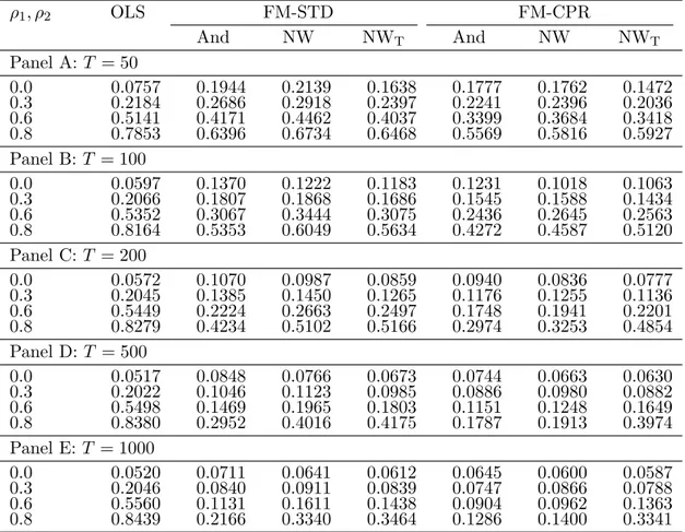
For our simulations we use exactly the same data generating processes (DGPs) as Wag- ner and Hong (2016, Section 3), i. e., we generate data for the quadratic cointegrating polynomial regression model:

y_t=c+δt+β₁x_t+β₂x²_t+u_t, (48) where the errorsut and vt= ∆xt are generated as:

u_t=ρ₁ut−1+ε_t+ρ₂e_t, u₀= 0, v_t=e_t+ 0.5et−1,

with (ε_t, e_t)⁰ ∼ N(0, I₂). The parameter ρ₁ controls the level of serial correlation in the error term ut, and ρ2 controls the extent of regressor endogeneity. The parameter values are set to c = δ = 1, β₁ = 5 and β₂ = −0.3. The values for β₁ and β₂ are based on coefficient estimates obtained by applying the FM-CPR estimator to GDP and CO2 emissions data for Austria (see Wagner, 2015). We present simulation results for T ∈ {50,100,200,500,1000} and for ρ₁ = ρ₂ ∈ {0,0.3,0.6,0.8}. The number of replications is 10,000 in all cases and all tests are carried out at the nominal 5% level.

We only report results for the Bartlett kernel, with the results for the Quadratic Spectral kernel, contained in supplementary material available upon request, qualitatively very similar. With respect to the bandwidth we report results for three choices. These are