Submarine permafrost map in the Arctic modeled
1
using 1-D transient heat flux (SuPerMAP)
2
P. P. Overduin1, T. Schneider von Deimling1, F. Miesner1, M. N. Grigoriev3,
3
C. D. Ruppel4, A. Vasiliev5, H. Lantuit1, B. Juhls6, and S. Westermann7
4
1Alfred Wegener Institute Helmholtz Centre for Polar and Marine Research (AWI), Potsdam, Germany
5
2Max Planck Institute, Hamburg, Germany
6
3Melnikov Permafrost Institute, Siberian Branch, Russian Academy of Sciences, Yakutsk, Russia
7
4U.S. Geological Survey, Woods Hole, MA, USA
8
5Earth Cryosphere Institute of Tyumen Scientific Center, Siberian Branch, Russian Academy of Sciences
9
and Tyumen State University, Tyumen, Russia
10
6Institute for Space Sciences, Freie Universit¨at Berlin, Berlin, Germany
11
7Geoscience Department, University of Oslo, Oslo, Norway
12
This is the peer reviewed version of the following article:
13
Overduin, P. P., Schneider von Deimling, T., Miesner, F.,Grigoriev, M.
14
N., Ruppel, C. D.,Vasiliev, A., et al. (2019). Submarine permafrost map
15
in the Arctic modeled using 1-D transient heat flux(SuPerMAP).
16
Journal of Geophysical Research: Oceans, 124,
17
which has been published in final form at
18
https://doi.org/10.1029/2018JC014675.
19
This article may be used for non-commercial purposes in accordance with
20
Wiley Terms and Conditions for Use of Self-Archived Versions.
21
Key Points:
22
• Submarine permafrost is modeled as 1D transient heat flux over multiple
23
glacial-interglacial cycles on the circumarctic shelf.
24
• Modeled permafrost ice content closely matches available geophysical
25
observations from the Beaufort and Kara Seas.
26
• Almost all modeled preindustrial submarine permafrost in the Arctic is
27
warming, thawing and thinning.
28
Corresponding author: P. P. Overduin,paul.overduin@awi.de
Abstract
29
Offshore permafrost plays a role in the global climate system, but observations of per-
30
mafrost thickness, state and composition are limited to specific regions. The current global
31
permafrost map shows potential offshore permafrost distribution based on bathymetry
32
and global sea level rise. As a first order estimate, we employ a heat transfer model to
33
calculate the subsurface temperature field. Our model uses dynamic upper boundary con-
34
ditions that synthesize Earth System Model air temperature, ice mass distribution and
35
thickness and global sea level reconstruction, and applies globally distributed geother-
36
mal heat flux as a lower boundary condition. Sea level reconstruction accounts for dif-
37
ferences between marine and terrestrial sedimentation history. Sediment composition and
38
pore water salinity are integrated in the model. Model runs for 450 ka for cross-shelf tran-
39
sects were used to initialize the model for circumarctic modeling for the past 50 ka. Prein-
40
dustrial submarine permafrost (i.e. cryotic sediment), modeled at 12.5 km spatial res-
41
olution, lies beneath almost 2.5×10⁶km2 of the Arctic shelf between water depths of
42
150 m bsf and 0 m bsf. Our simple modeling approach results in estimates of distribu-
43
tion of cryotic sediment that are similar to the current global map and recent seismically-
44
delineated permafrost distributions for the Beaufort and Kara seas, suggesting that sea
45
level is a first-order determinant for submarine permafrost distribution. Ice content and
46
sediment thermal conductivity are also important for determining rates of permafrost
47
thickness change. The model provides a consistent circumarctic approach to map sub-
48
marine permafrost and to estimate the dynamics of permafrost in the past.
49
1 Introduction
50
Permafrost is defined as Earth material with a perennially cryotic (<0◦C) temper-
51
ature (van Everdingen, 1998). Submarine (or subsea or offshore) permafrost is permafrost
52
overlain by a marine water column. Most submarine permafrost occurs in the Arctic (Brown
53
et al., 2001), is relict terrestrial permafrost (Romanovskii et al., 2004; Kitover et al., 2015)
54
and has been degrading since being inundated during sea level rise starting after the Last
55
Glacial Maximum (Osterkamp, 2001). Submarine permafrost may or may not contain
56
ice (i.e. be partially frozen), depending on its temperature, salt content, sediment grain
57
size and composition. While important to coastal and offshore processes and infrastruc-
58
ture (Are, 2003), recent attention has focused on its role in the global carbon cycle. Large
59
amounts of fossil organic carbon (McGuire et al., 2009) and greenhouse gases (Shakhova
60
& Semiletov, 2007) may exist intrapermafrost and/or subpermafrost. Ruppel (2015) es-
61
timates that 20 Gt C (2.7×10¹³kg CH4) may be sequestered in gas hydrates associated
62
with permafrost, mostly in Arctic Alaska and the West Siberian Basin. Methane in par-
63
ticular may be present in large amounts in gas hydrate form (e. g. Dallimore & Collett,
64
1995) and be destabilized by permafrost thaw (e. g. Frederick & Buffett, 2015), although
65
methane emissions may be oxidized before reaching the atmosphere (Overduin et al., 2015;
66
Ruppel & Kessler, 2017) or better explained by geological sources (Anisimov et al., 2014).
67
Given projected future decreases in sea ice cover, thickness and duration on the Arctic
68
shelves, water temperatures are expected to rise at an increasing rate, increasing heat
69
transfer to shelf sediments and accelerating submarine permafrost thaw. The release of
70
stabilized, contained or trapped greenhouse gases from submarine permafrost is thus a
71
potential positive feedback to future climate warming.
72
Most submarine permafrost is relict permafrost that has developed where glacia-
73
tion, climate and relative sea level fluctuation permit terrestrial permafrost to be trans-
74
gressed by rising sea level. Large warm-based glacial ice masses during cold climate pe-
75
riods prevented permafrost from forming. We thus expect submarine permafrost on the
76
continental shelf regions that were not glaciated: most of the shelves of the marginal seas
77
of Siberia (Kara, Laptev, East Siberian, Chuckhi) and the Chukchi and Beaufort Sea of
78
North America. The International Permafrost Association (IPA) permafrost map (Brown
79
et al., 2001) shows submarine permafrost based on global sea level reconstructions, mod-
80
ern bathymetry and the assumption that permafrost persists out to about the 100 m iso-
81
baths. Existing maps focus on the regional scale (Vigdorchik, 1980b,a; Nicolsky et al.,
82
2012; Romanovskii et al., 2004; Zhigarev, 1997) and are based on different combinations
83
of theoretical and empirical approaches to simulate permafrost evolution over time. Some
84
of these tend to reproduce coverage similar to the IPA map, with some combination of
85
cryotic and ice-bonded permafrost, for example for the Laptev Sea (Romanovskii et al.,
86
2004; Tipenko et al., 1999; Nicolsky et al., 2012) whereas other models produce a more
87
conservative estimate of isolated regions of near-shore ice-bonded permafrost (Zhigarev,
88
1997).
89
Nicolsky et al. (2012) and Lachenbruch (1957, 2002) demonstrate that thermokarst
90
lakes, rivers and saline sediments can form ice-poor regions within millennia after trans-
91
gression. Nonetheless, the Last Glacial period and continental climate of eastern Siberia
92
led to particularly cold and deep permafrost over a broad expanse of continental shelf,
93
permafrost that persists until today. Publicly available observational data are limited
94
to shallow boreholes drilled from ships (Kassens et al., 1999; Rekant et al., 2015) or from
95
the sea ice (S. Blasco et al., 2012; Dallimore, 1991; Winterfeld et al., 2011), a few deeper
96
scientific boreholes, geophysical records from industrial boreholes in the Beaufort Sea (e. g.
97
Hu et al., 2013) and geophysical records (e. g. Portnov et al., 2016; Rekant et al., 2015).
98
Data from boreholes deep enough to penetrate permafrost in the prodeltaic region of the
99
Mackenzie River and on the Alaskan Beaufort shelf have been published and analyzed
100
for the depth of the base of permafrost (Issler et al., 2013; Hu et al., 2013; Brothers et
101
al., 2016; Ruppel et al., 2016). Relating geophysical observations to permafrost depth,
102
lithology, cryostratigraphy or sediment temperature is not trivial. Hu et al. (2013) ex-
103
amine over 250 borehole records, including over 70 offshore boreholes, and find permafrost
104
100 to 700 m thick north of the Mackenzie Delta and eastward. Ruppel et al. (2016) and
105
Brothers et al. (2016) analyze available borehole and seismic data from the U.S. Beau-
106
fort Sea to provide a conservative representation of permafrost extent on the shelf: it is
107
restricted to waters less than 20 m deep and closer than 30 km from shore.
108
Thus, regional modeling efforts and observational studies differ, suggesting an in-
109
complete understanding of permafrost dynamics on the shelf, and observations suggest
110
significant spatial variability at the regional to circumarctic scale. Given its potential
111
role in storing methane and mitigating its emission, and given that the Arctic shelf seas
112
are undergoing unprecedentedly rapid changes, understanding of this component of the
113
global climate system is important. A globally consistent model of submarine permafrost
114
evolution may explain its distribution and vulnerability to the changes currently under-
115
way in the Arctic. Such a first-order model can be tested by evaluating whether its re-
116
sults match available observations of subsea permafrost in terms of presence vs. absence,
117
lateral and depth extents, and ice content. An evaluation of the sensitivity of these out-
118
put parameters to input data sets can provide clues as to which improvements are re-
119
quired for better predictive capacity at specific sites.
120
The objective of this study is to use available circumarctic data sets to model the
121
thermal dynamics of Arctic shelf sediments at the circumarctic scale over multiple glacial-
122
interglacial cycles using a simple first-order model. We hypothesize that submarine per-
123
mafrost is widespread wherever a lack of glaciation permitted deep and cold permafrost
124
to form during the Late Pleistocene, and that degradation since the Holocene has reduced
125
much of this once deeply frozen permafrost to ice-poor permafrost.
126
2 Method
127
2.1 Modeled domain
128
We used CryoGrid 2, a 1-D heat diffusion model introduced by Westermann et al.
129
(2013). For the purpose of simulating the thermal state of Arctic shelf regions we have
130
modified and extended the current model in various aspects that we describe in the fol-
131
lowing.
132
We focussed on the Arctic shelf between modern isobaths of 0 and 150 m below sea
133
level (m bsl) (the pink region in Figure 1). Modeling was performed on a 7000×7000
134
km grid of 560×560 equidistant points at 12.5 km spacing in the northern polar EASE
135
Grid 2.0 format (Brodzik et al., 2012, 2014). Elevation or bathymetry was averaged for
136
each 12.5 km grid cell from the International Bathymetric Chart of the Arctic Ocean (IB-
137
CAOv3.0) (Jakobsson et al., 2012). Of the resulting 313 600 grid cell centers, 43 459 (6.79×10⁶km2)
138
lay between 0 and 150 mbsl. Of these, we removed cells the Baltic, surrounding Iceland,
139
in the southern Bering Strait, in the Ob estuary and Lena River channel, and all points
140
south of 65◦N, leaving a set of 26 333 grid cells covering an area of 4.11×10⁶km2. Ther-
141
mal modeling was performed below the ground surface (corresponding to the sea bed,
142
the land surface or the sub-glacial surface) to a depth of 6000 m. Modeled locations were
143
grouped based on Arctic shelf seas as defined by the preliminary system of the Interna-
144
tional Hydrographic Organisation, modified to extend to the north pole (IHO, 2002, the
145
blue polygons shown in Figure 1 ).
146
Conductive heat flow below the Earth surface was modeled based on the continu- ity equation for internal energyE (in J m−3)
∂E
∂t + ∂
∂zFheat. (1)
We denote the time witht(in s) and the vertical coordinate withz (in m). The conduc- tive heat flux is given by
Fheat=−k(z, T)∂T
∂z, (2)
wherekdenotes the thermal conductivity (in W m−1K−1). Expanding the time deriva- tive of equation (1) as the partial derivatives ofT and introducing the water contentθw
(expressed as volume fraction), we obtain
∂E
∂t =∂E
∂T
∂T
∂t + ∂E
∂θw
∂θw
∂T
∂T
∂t. (3)
This can be further reduced with the volumetric heat capacityc= ∂E∂T and and the la- tent heat of freezing and melting of water and iceLf = ∂θ∂E
w to the one-dimensional heat equation
c(z, T) +Lf
∂θw
∂T ∂T
∂t − ∂
∂z
k(z, T)∂T
∂z
= 0. (4)
To simplify, the sensible and latent heat terms can be combined to the effective heat ca- pacityceff
ceff(z, T) =c(z, T) +Lf
∂θw
∂T , (5)
(in J m−3K−1). The modifications and additions that we introduced to the main model
152
from Westermann et al. (2013) are described in the following sections.
153
2.2 Ice content and sediment type
154
Sediment thermal properties depend on sediment grain size and porosity, temper- ature and the concentration of dissolved solids in the pore water. In our model, the lat- ter depends on whether the depositional environment is terrestrial or marine. In order to be able to solve equation (4) we need to obtain an equation for the effective heat ca- pacity and in particular solve ∂θ∂Tw. To determine the freezing temperature of the pore solution and the liquid water content, we calculate the effect of the solutes on the wa- ter potential as a function of temperature. Ma et al. (2015) give the generalized Clausius- Clapeyron equation as
1 ρw
− 1 ρi
u=Lf
T−Tf0
Tf0 , (6)
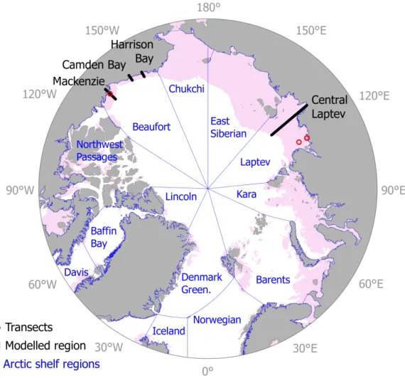
Figure 1. The modeled domain includes Arctic shelf regions with modern water depths less than 150 m (shaded pink). Black points indicate locations modeled for 450 ka runs (Figure 6).
Blue lines show the preliminary classification of the Arctic Ocean following the International Hydrographic Organisation (IHO, 2002), which has been modified to extend to the pole in order to include the entire shelf region. Sites for model sensitivity are marked as red circles.
147 148 149 150 151
whereuis pressure (in Pa),ρw andρiare the densities of liquid water and ice (in kg m−3), Lf is the latent heat of fusion for water (in J kg−1), andT andTf0are the temperature and the freezing temperature of free water (in K). This assumes the equilibrium case where u = uw = ui, withuwandui being the gauge pressures of water and ice. When so- lutes are present in the pore water, an osmotic pressure or potential term,
Π =R T C, (7)
is introduced (Loch, 1978; Bittelli et al., 2003), whereR is the universal gas constant (in 8.3144 J K−1mol) andC is the solute concentration in the pore solution (in mol m−3).
Thus, equation (6) changes to
uw−Π ρw
−ui ρi
=LfT−Tf Tf
, (8)
which describes a depression of the temperature at which freezing begins. The freezing point is
Tf =Tf0−RTf02 Lf
N (9)
whereN is the normality of the solution in equivalents per liter. N can be related to the salinity of the overlying seawater,S, via
N = 0.9141S(1.707×10⁻²+ 1.205×10⁻⁵S+ 4.058×10⁻⁹S2) (10) based on Klein & Swift (1977) or to molarity,M, of a salt solution via
N = M
feq, (11)
wherefeq is the numbers of equivalents per mole of solute. From equation (8), ignoring the difference in densities of water and ice, the resulting expression for the soil water pres- sure becomes
uw(T, θw, ns) = Lf
ρw
T−Tf
Tf
−RN T ρw
1 θsat − 1
θw
(12) forT < Tf, and is relative to solute concentration in the total pore space. We use the van Genuchten-Mualem formulation for soil water potential based on the correspondence between drying and freezing, to obtain the freezing characteristic curve as a function of temperature and solute concentration
θw(T, ns) =θsat
1 +
− α
ρwguw(T, θw) n1-nn
, (13)
whereαand n are sediment-dependent Van Genuchten parameters (Dall’Amico et al.,
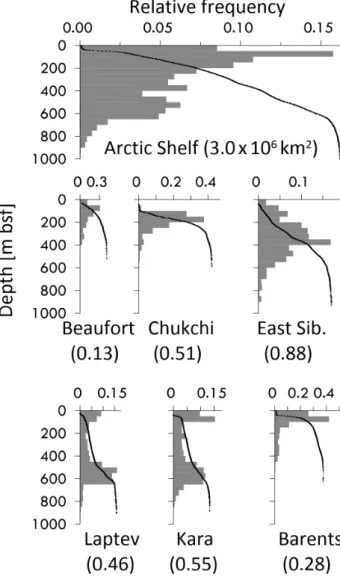
155
2011), andgis the gravitational constant. Equation (13) gives the liquid water content
156
for differing sediment types as a function of freezing temperature and salinity. Freezing
157
characteristic curves give the unfrozen water content of the sediment as a function of tem-
158
perature. A comparison of measured (Hivon & Sego, 1995; Overduin et al., 2008) and
159
modeled unfrozen water content is shown in the supporting information (Figure S1). For
160
measured values, salinity was converted to molality using the TEOS-10 toolbox (Millero
161
et al., 2008) for the valences and atomic weight of dissolved salts in seawater or NaCl.
162
2.3 Stratigraphy
163
The thickness of sedimentary deposits and their compaction determine porosity and
164
are thus important for pore space and ice content in permafrost. Global maps of total
165
sediment thickness of the oceans and marginal seas based on geophysical observations
166
are available (e.g. Whittaker et al., 2013). This data set (NGDC) demonstrates one of
167
the challenges of working in the Arctic, namely the paucity of available data: the map
168
covers everything except for the Arctic Ocean and its shelf seas. Sediment thickness along
169
the coasts varies spatially, with high thicknesses where rivers terminate and where glacial
170
outwash contributed to sedimentation (Jackson & Oakey, 1990). Submerged valleys drain-
171
ing the shelf can have locally high rates of sedimentation (Kleiber & Nissen, 2000; Bauch
172
et al., 2001). On the Arctic shelf, sedimentation associated with deglaciation also con-
173
tributes to this variability (e.g. Batchelor et al., 2013). This spatial variability implies
174
a temporal variability associated with tectonics, sea level change and glacial dynamics.
175
Rates of sedimentation are typically higher during deglaciation (Bauch et al., 2001) and
176
vary with distance from the coast (Kuptsov & Lisitzin, 1996).
177
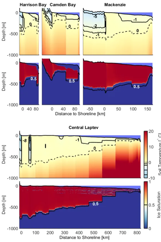
To simulate the effect of repeated transgression on stratigraphy, sediment proper-
178
ties were initialized based on parameterization for marine and terrestrial sediments. Ob-
179
served linear sedimentation rates for the Arctic shelf region are highly variable. Long term
180
mean linear sedimentations rate on the shelf are typically on the order of meters per mil-
181
lion years, within the range given by Gross (1977) for both marine and terrestrial sed-
182
imentation rates and subglacial sediment dynamics (Boulton, 1996). The range of lin-
183
ear sedimentation rates inferred from surface sediment records across the Laptev Sea shelf
184
range from near zero during the Holocene to over 2.5 cm/ka close to the shelf edge (Bauch
185
et al., 2001). Viscosi-Shirley et al. (2003) report rates based onδ14C and210Pb dating
186
of sediment cores of between 2–70 cm/ka for Laptev Sea and 200–700 cm/ka for the Chukchi
187
Sea. In both cases the origin of the sediment is over 60 % terrigenous or riverine. Kuptsov
188
& Lisitzin (1996) find sedimentation rates of 11–160 cm/ka for the inner Laptev Sea. We
189
choose transgressive and regressive sedimentation rates of 30 cm/ka and 10 cm/ka, re-
190
spectively, for the entire shelf region, for circumarctic modeling. The salinity of pore wa-
191
ter in marine sediment was set to 895 mol m−3. The resulting freezing characteristic curves
192
are shown in the supporting information (Figure S1).
193
This treatment of sediment dynamics ignored spatial variation in sedimentation rate
194
across the shelf and along the continental margin. By back-calculating sediment accu-
195
mulation during transgressive and regressive periods, onlapping marine transgression sed-
196
iment strata and disconformities were created within the model domain, which affected
197
the amount of ice frozen during sea level low-stand ground cooling. In transgressive en-
198
vironments, terrestrial strata typically terminate with an erosional marine ravinement
199
surface called a transgressive nonconformity (Forbes et al., 2015). Such alternating ter-
200
restrial and marine sediment layers are strongly suggested by the few cored and well-described
201
offshore cores on the Arctic shelf, which encounter alternating strata of saline and fresh-
202
water permafrost (e.g. S. M. Blasco et al., 1990; Rachold et al., 2007; Ponomarev, 1940,
203
1960). These alternations are not generally visible in offshore permafrost temperature
204
records, which are typically near-isothermal (Lachenbruch, 1957) but are often suggested
205
by sediment structure visible in geophysical records (e.g. Batchelor et al., 2013; Ruppel
206
et al., 2016). This representation ignores possible deeper variations in salinity due to ground-
207
water or freezing that have been assumed in other models (e.g. salinity increases to 30%
208
at 10 km depth in Hartikainen & Kouhia, 2010).
209
Coastal erosion and landward migration of the coast associated with transgressions
210
lead to an increase in the elevation of the base level for the Arctic coastal plains. The
211
sedimentary regime landward of the coast is therefore either low or negative. Although
212
differences between regressive and transgressive sediments are accommodated in Cryo-
213
Grid 2, the model does not yet account for erosion, which, under subaerial conditions,
214
can include denudation and thermokarst processes, prior to transgression.
215
In addition to alternation between transgressive and regressive sedimentation regimes, sediment compaction is an important inuence on sediment porosity and thus partially controls sediment ice content. Porosity usually decreases with depth depending on grain geometry, packing, compaction, and cementation (Lee, 2005) and usually changes at the boundary between unconsolidated and unconsolidated material. Available models of sed- iment bulk density or compaction are often empirical and based on global deep-sea databases
(Gu et al., 2014; Hamilton, 1976; Kominz et al., 2011). The porosity-depth relationship by Lee (2005) ranges from 0.53 at the seafloor to 0.29 at 1200 m below the sea floor (bsf), based on five wells from Milne Point in Prudhoe Bay, Alaska. Gu et al. (2014) combine observations of sediment bulk density for the upper-sediment and lower-sediment com- paction from 20 347 samples down to depths of 1737 m bsf. Extrapolation to depth leads to a porosity of less than 5 % at depths greater than 1.2 km. We applied an exponential decrease in porosity from a surface porosity of 0.4 to 0.03 at 1200 m depth, fit to dry bulk density data from Gu et al. (2014) for the shallow Arctic shelf:
η = 1.80ρ−1b −0.6845. (14)
A comparison of porosity profiles over depth is presented in the supporting information
216
(Figure S2). The employed parametrization of sediment porosity and pore water salin-
217
ity must be considered a first-order approximation which should be refined. The high
218
variability of sediment column thickness found on the shelf, the high proportion of glacially,
219
fluvially and alluvially deposited terrigenous material and the presence of transgressive
220
unconformities may lead to shelf sediment columns that differ from those recorded in ma-
221
rine drilling databases. Our approach represents compaction and the influence of trans-
222
gressive and regressive cycles, but cannot describe the spatial variability of geological struc-
223
tures on the Arctic shelf.
224
2.4 Boundary conditions
225
Permafrost evolution was driven by upper and lower boundary conditions on the modeling domain (0–6000 m below the surface). This condition was a warming or cool- ing of the underlying ground via changing surface temperature from above and via geother- mal heat flux from below. For the latter, we used the global data set from Davies (2013)[][and supporting information (Figure S3)], based on area-weighted medians of measurements from a global heat flow data set of over 38 000 measurements correlated to geology
Fheat(t,6000 m) =−Q, (15)
whereQis the geothermal heat flux (in W m−2). For the former, surface conditions at each modeled time and location were defined as subaerial, submarine or subglacial de- pending on modern land surface elevation and bathymetry (Jakobsson et al., 2012), sea level reconstruction (Grant et al., 2014) and glacial ice cover (Ganopolski et al., 2010):
T(t,0 m) =
Tsurf ace for subaerial Tbenthic for submarine Tbasal for subglacial.
(16)
In the runs described in this study, we have used spatially explicit surface temperature
226
records simulated by the intermediate complexity Earth System Model CLIMBER-2 (Ganopol-
227
ski et al., 2010), which also provides glacial ice cover extent and thickness. For this pur-
228
pose we have interpolated the climate model data (with a resolution of 10◦ in latitude
229
and 51.4◦ in longitude) to modeled locations. The mean ground surface temperature and
230
the probability distribution about this median for the modeled domain are shown in Fig-
231
ure 2.
232
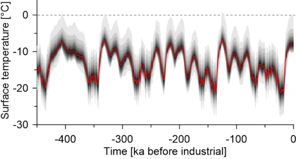
The mean surface temperatures over 450 ka at each modeled location ranged be-
233
tween−17.7◦C and 0◦C with a mean of−7.3◦C in the modeled domain. An animation
234
of sea level, ice cap distribution and the modern coastline is available in the supporting
235
information. Deglacial periods and concomitant transgressions are rapid (<10 ka) com-
236
pared to regressive periods. The area of shelf exposed to subaerial conditions therefore
237
varies over time and space, so that cumulative exposure of the shelf to subaerial condi-
238
tions increases toward the modern coastline. Given extreme values for mean surfacing
239
temperature forcing (−31.9◦C, 0◦C), geothermal heat flux (55.7 W m−2, 132.6 W m−2)
240
Figure 2. Mean subaerial ground surface temperature forcing data for the past 450 ka from the CLIMBER-2 model (Ganopolski et al., 2010). The gray shaded region around the mean gives the 95 % confidence limits in 5 % steps for the spatial variability in surface temperature for the set of modeled EASE Grid 2.0 locations.
243 244 245 246
and sediment stratigraphy (uniformly marine or terrestrial), steady state permafrost thick-
241
nesses ranged from 0 m bsf to 658 m bsf and 1675 m bsf.
242
There are no regional sea level reconstructions for Arctic shelf seas (Murray-Wallace
247
& Woodroffe, 2014), although many studies provide records of the Holocene transgres-
248
sion (Bauch et al., 2001; Brigham-Grette & Hopkins, 1995). We used the global scale
249
sea level reconstruction from Grant et al. (2014) which covers five glacial cycles based
250
on Red Sea dust and Chinese speleothem records. Inferred ice volumes from any global
251
sea level reconstruction do not necessarily agree with modeled ice volumes provided by
252
CLIMBER-2 output. Our model does not explicitly require ice volume, but uses glacial
253
extent to define the upper temperature boundary condition for the modeled permafrost.
254
By insulating the ground against cold surface air temperatures, thick glacial ice masses
255
influence the temperature regime of subglacial sediments. Ice sheet thicknesses from CLIMBER-
256
2 on a latitude-longitude grid of 0.75◦×1.5◦ were interpolated to EASE Grid 2.0 res-
257
olution, based on the same simulation setup as used for surface air temperatures. We
258
assume a mean annual subglacial temperature of 0◦C, corresponding to warm-based ice
259
masses. Thinner ice sheets can be effective at conducting heat and are more likely to be
260
cold-based, so that CLIMBER-2 ice masses less than 100 m thick were not included. When
261
ice mass distribution extended to regions lying below sea level, we assumed grounding
262
zone and assigned a subglacial temperature.
263
Once transgressed, cold terrestrial sediments are warmed by the overlying sea wa-
264
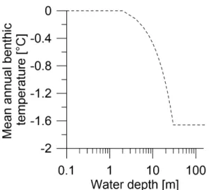
ter. Forcing temperature at the seabed was set as a function of water depth (Figure 3).
265
In the model, the mean annual benthic temperature was set to 0◦C from the shoreline
266
to 2 m water depth. Between 2 and 30 m, the mean annual benthic temperature decreased
267
linearly from 0◦C to the freezing temperature of sea water. Beyond this depth and to
268
the edge of the shelf a constant benthic temperature was assumed. This results in ben-
269
thic temperatures as a function of water depth that are comparable to the approach of
270
Figure 3. For submarine periods, the upper boundary condition was the benthic water tem- perature, which was defined as a function of water depth on the Arctic shelf.
285 286
Nicolsky et al. (2012), based on observational data collected over almost a century from
271
the Siberian shelf region (Dmitrenko et al., 2011). This parameterization does not in-
272
clude the possible thermal coupling of the seabed to the atmosphere in winter through
273
bedfast ice. At water depths less than the maximum thickness of sea ice, bottom-fast
274
sea ice may form, thermally coupling the seabed to the atmosphere and leading to mean
275
annual benthic water temperatures as low as−6◦C in shallow water (Harrison & Os-
276
terkamp, 1982; Soloviev et al., 1987). Since this effect is only observed in nearshore shal-
277
low water, it probably does not play a role at the temporal and spatial scales modeled
278
here. The influences on benthic temperatures of oceanic currents, stratification, and most
279
importantly riverine and world ocean inflow onto the shelf were not included.
280
Given the large spatial extent of the circumarctic shelf region and the fact that we
281
have ignored important processes that affect whether a modeled location was subaerial,
282
subglacial or submarine (e.g. neotectonics, isostasy), the modeled paleo-evolution of per-
283
mafrost was a first order estimate.
284
2.5 modeling
287
Two model runs were executed, one for selected transects crossing the Arctic shelf
288
from the coast to the 150 m isobath (Figure 1) and a run for the circumpolar Arctic shelf.
289
Transects were modeled for 450 ka using a steady state temperature profile as initial con-
290
dition, calculated for the sediment profile using the surface temperature and geothermal
291
heat flux as boundary conditions. The circumpolar domain was modeled for 50 ka, ini-
292
tialized with a steady state temperature profile at 50 ka at each modeled location for the
293
first time-step. The steady-state solution was calculated based on the temperatures at
294
the lower boundary,T(t, z) =T(50 ka,2000 m), and the surface,T(50 ka,0 m), at the first
295
time step of the model run. Values for the temperatures at 2 km were derived from a cor-
296
relation ofT(t,2000 m) with the geothermal heat flux and cumulative surface temper-
297
ature forcing for 153 locations along 6 transects (Figure 1) from 450 ka to 50 ka:
298
T(50 ka,2000 m) = 712.1Q+ 3.312×10⁻⁴
50 ka
X
450 ka
Tsurf(t,0 m) + 2.076 (17)
for which the correlation coefficient wasR2= 0.99 with a standard deviation of the resid-
299
uals of less than 1.5◦C.
300
The CryoGrid 2 model produces the subsurface temperature fieldsTs(t, z) for each
301
modeled location from the ground surface or sea bed down to 2 km below the surface.
302
From these data, together with the profile of sediment characteristics, the depth to the
303
lowermost 0◦C isotherm,zPf(in m), the fractional liquid water content θw(t, z), the ice
304
content of the sediment columnθi(t, z) (in m3m−2) and the enthalpy of freezingHf(t, z)
305
(in MJ m−2) for each subsurface grid cell can be calculated. We define permafrost as cry-
306
otic (<0◦C) sediment, regardless of ice content, matching the accepted western defi-
307
nition for terrestrial permafrost (van Everdingen, 1998). Such thermally-defined permafrost
308
is not necessarily useful as an indication of past climate or of permafrost response to fu-
309
ture climate. Ice content is more important than temperature in terms of the functions
310
of permafrost: providing thermal inertia to perturbation, reducing gas fluxes, and sta-
311
bilizing gas hydrates; and in terms of observing permafrost using geophysical methods.
312
Seismic methods will only delineate ice-bonded permafrost; permafrost containing lit-
313
tle to no ice will not have the elevated propagation velocity needed for seismic refrac-
314
tion or reflection detection. For validation purposes, model output of ice content can match
315
penetration depths of available observational data. The enthalpy is calculated as the sum
316
of the energy requirements for warming the sediment column to its freezing temperature
317
and for thawing of the ice (Nicolsky & Romanovsky, 2018) and indicates the energy re-
318
quired to reach a permafrost-free sediment column.
319
To evaluate sensitivity of model output to parameterization, 4 grid cells were se-
320
lected (see supporting information Tab. 1, and Figure 1) from the Beaufort and West-
321
ern Laptev seas. The selected sites represent the full ranges of relative transgressive/regressive
322
sedimentation regimes, and of subaerial/ submarine surface forcing. At these sites we
323
varied (i) the model parameterization, (ii) the initial conditions, and (iii) the forcing data,
324
as listed in the supporting information (Tab. 2) for 450 ka. We then analyzed how these
325
variations changed the modeled lower permafrost boundary (i.e. 0◦C isotherm).
326
3 Results
327
3.1 Circumarctic Submarine Permafrost Distribution
328
Submarine permafrost evolution was simulated using vertical conductive heat flux
329
for the Arctic shelf region with modern elevations between 150 and 0 m bsl and linear
330
sedimentation rates for regressive and transgressive regimes of 10 cm/ka and 30 cm/ka,
331
respectively, mineral conductivity of 3 W m−1K−1, and initialization with equilibrium
332
conditions at 50 kaBP for a subset of cross-shelf transects. The resulting preindustrial
333
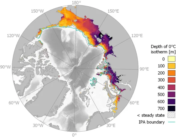
spatial distribution of submarine permafrost and the depth of the 0◦C isotherm below
334
the seafloor are shown in 4. Submarine permafrost in Figure 4 is cryotic sediment that
335
was exposed subaerially at some point during the past 450 ka and that exceeds the pen-
336
etration depth of the 0◦C isotherm under modern assumed benthic temperatures (Fig-
337
ure 3 ), with a tolerance of 50 m. The latter condition excludes Holocene permafrost at
338
the sea bed at temperatures higher than the freezing point of sea water (the region so
339
excluded is shown in Figure 4). Submarine permafrost is unevenly distributed around
340
the circumpolar shelf, with almost all modeled cryotic sediment distributed on the shelf
341
east of 60◦E and west of 120◦W. Within each shelf sea, the cryotic permafrost thick-
342
ness was generally greatest at the most recently submerged region, usually at the coast,
343
and decreased northward toward the shelf edge (Figure 4).
344
preindustrial submarine permafrost underlays more than 80 % of five Arctic seas:
345
the Beaufort, Chukchi, East Siberian, Laptev and Kara seas (Tab. 1). Of these the Kara,
346
Laptev and East Siberian Seas also have mean permafrost thicknesses exceeding 300 m bsf.
347
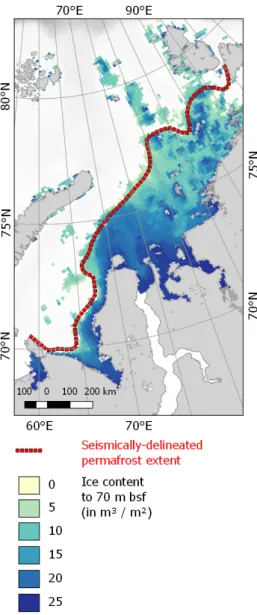
Thus, the greatest spatial extent of permafrost underlies this region, which, together with
348
Figure 4. The distribution of modeled postindustrial cryotic sediment and the depth of the lower 0◦C isotherm beneath the Arctic Ocean Shelf seas. Modern Arctic Ocean bathymetry (Jakobsson et al., 2012) and land masses are shown. Submarine permafrost extent from the In- ternational Permafrost Association’s map is indicated as a cyan line (Brown et al., 2001). In the hatched region, assumed modern sea floor temperatures produce permafrost exceeding modeled depths by more than 50 m.
365 366 367 368 369 370
the adjacent Chukchi Sea, comprises more than 60 % of the modeled region. In the Cana-
349
dian Arctic Archipelago, which includes the Lincoln Sea, Baffin Bay, part of the Davis
350
Strait and the Northwest Passages (Figure 1), modeled permafrost underlay 23 % of the
351
modeled region, and 5 % of the shelf sea region. Grid cells with permafrost in the Cana-
352
dian Arctic Archipelago, with the exception of the Beaufort coast (which is included in
353
the Beaufort Sea region), were located adjacent to the coast. A similar distribution was
354
found in the Barents Sea, where cryotic sediments underlay 57 % of the modeled region
355
(restricted to water depths of maximally 150 m), but only 19 % of the sea’s total area.
356
Cryotic sediment in the Barents Sea was located primarily in two regions: south of Sval-
357
bard and along the coast, from around the Kanin Peninsula in the west to Novaya Zemlya.
358
In the Kara Sea, permafrost distribution was strongly skewed towards the eastern por-
359
tion of the sea, including Baydaratskaya Bay, a narrow strip less than 100 km wide along
360
the western coast of the Yamal Peninsula, and the region northeastward towards Sev-
361
ernaya Zemlya. Contiguous regions with permafrost exceeding 500 m bsf in thickness were
362
restricted to this portion of the Kara Sea, the Laptev Sea and portions of the East Siberia
363
Sea surrounding the New Siberian Islands.
364
3.2 Permafrost Thickness
371
Figure 5 shows histograms of the depth of the lower 0◦C isotherm below the seafloor
372
for the Arctic shelf and for six of the shelf seas. Assuming that cryotic sediments extend
373
from the seabed to this lower depth, hypsometric curves describe the cumulative exceedance
374
functions for each shelf sea. Cryotic sediment was generated between 0 and 1117 m bsf
375
(depth of 0◦C isotherm). Half of the values lay between 160 and 470 m bsf (Figure 5),
376
with a mean depth of cryotic sediment of 287 m bsf. For the Arctic shelf, the most fre-
377
quent permafrost thickness was less than 200 m, but for individual seas, distributions of
378
thickness varied. The seas accounting for the greatest area of the modeled permafrost
379
(Kara, Laptev and East Siberian) had peaks of permafrost thickness at greater depths
380
(around 600, 600 and 400 m, respectively) than the other shelf regions. The depth of the
381
0◦C isotherm was shallow (<100 m bsf) in the Svalbard region and in the southeastern
382
Barents Sea, except at its easternmost extent in Varandey Bay, where it exceeded 250 m bsf
383
and where the IPA map also indicates a small region of submarine permafrost. Modeled
384
submarine permafrost reached its greatest depth (1117 m bsf) in the Canadian Arctic Archipelago.
385
Model sensitivity to variation of input parameters was tested for individual param-
386
eters with lower permafrost boundary depths of 255 m bsf, 617 m bsf, 601 m bsf and 541 m bsf
387
at the Beaufort Sea and western Laptev Sea sites, respectively. The depth to the lower
388
boundary of cryotic sediment changed by more than 100 m for imposed changes in 2 pa-
389
rameters only: subaerial forcing temperature (varied by±5◦C) and sediment mineral
390
thermal conductivity (from−67 % to 2.33 %). Decreasing air temperatures uniformly by
391
5◦C increased permafrost thicknesses by 78 % and 32 to 37 %, for the Beaufort and the
392
three western Laptev sites, respectively. An increase in mineral thermal conductivity from
393
3 to 5 W m−1K resulted in 170 m (67 %) thicker permafrost at the Beaufort site and 300 m
394
to 350 m (around 55 %) at the western Laptev sites. For all other parameters (sea level:
395
±40 m, sedimentation rate: 10–60 cm/ka, depositional regime: 0–100 % marine, marine
396
sediment salinity: ±10 %, porosity: ±30 %, subglacial forcing: −5 to 0◦C and geother-
397
mal heat flux: ±10 %), changes were less than 100 m (see supporting information, Tab.
398
S2).
399
3.3 Permafrost Temperature and Temporal Variability
407
For particular transects extending northward from the coast, we describe model
408
results for the temporal development of modeled submarine permafrost for 2D cross-sections
409
of the shelf. Results give insights into (i) the behaviour of the model, (ii) the dependence
410
of submarine permafrost extent and composition on transient forcing and (iii) the im-
411
portance of modeled processes in determining modern permafrost distribution. Transects
412
were chosen to reflect the diversity of paleoenvironmental histories around the Arctic shelf
413
and to correspond to previous modeling efforts and/or potential observational data sets.
414
Table 2 lists the transects and their characteristics, as well as any references with sim-
415
ilarly located modeling or observational results.
416
Figure 6 shows modeled modern temperature and ice content distribution as a func-
417
tion of lateral distance from the coast with modern bathymetry and elevation. The pro-
418
files presented here run northward from onshore positions, where terrestrial permafrost
419
(at left in each profile) gives an indication of pre-transgression permafrost temperature,
420
thickness and ice content. The profiles extend out to 150 m water depth. The Harrison
421
Bay (HB) and Camden Bay (CB) profiles transect the Alaskan Beaufort coastline, where
422
Ruppel et al. (2016) analyze borehole records. The Mackenzie (MP) profile transects the
423
Canadian Beaufort coastline 140 km northeast of Tuktoyaktuk and extends more than
424
150 km offshore, where Taylor et al. (2013) model permafrost evolution. The central Laptev
425
Sea (CL) profile was located just east of the Lena Delta where the shelf extends over 800 km
426
northward from the coastline. Animations of sediment temperature and ice saturation
427
as a function of time are available in the supporting information.
428
Figure 5. Histograms show the relative frequency of grid cells with cryotic sediment within the main Arctic shelf seas classified by the depth of the lower permafrost boundary beneath the sea floor. The x-axes of the histograms are scaled proportionally to the number of grid cells so that the histogram areas are comparable. The area of cryotic sediment modeled within each shelf sea (in 106km2) are indicated in parentheses.
402 403 404 405 406
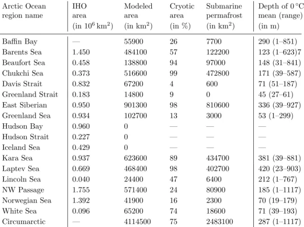
Arctic Ocean region name
IHO area
Modeled area
Cryotic area
Submarine permafrost
Depth of 0◦C mean (range) (in 106km2) (in km2) (in %) (in km2) (in m)
Baffin Bay — 55900 26 7700 290 (1–851)
Barents Sea 1.450 484100 57 122200 123 (1–623)7
Beaufort Sea 0.458 138800 94 97000 148 (31–841)
Chukchi Sea 0.373 516600 99 472800 171 (39–587)
Davis Strait 0.832 67200 4 600 71 (51–187)
Greenland Strait 0.183 14800 9 0 45 (27–61)
East Siberian 0.950 901300 98 810600 336 (39–927)
Greenland Sea 0.934 102700 13 3000 53 (1–299)
Hudson Bay 0.960 0 — — —
Hudson Strait 0.227 0 — — —
Iceland Sea 0.429 0 — — —
Kara Sea 0.937 623600 89 434700 381 (39–881)
Laptev Sea 0.669 468400 98 402700 420 (23–903)
Lincoln Sea 0.040 24400 47 6400 212 (1–767)
NW Passage 1.755 571400 24 80900 185 (1–1117)
Norwegian Sea 1.392 41900 16 2300 70 (19–179)
White Sea 0.096 65200 74 18600 71 (39–193)
Circumarctic — 4114500 75 2483100 287 (1–1117)
Table 1. Distribution of Shelf Areas and Regions Underlain by Cryotic Sediment Categorized Using a Modified Preliminary Classification of the Arctic Shelf Seas (IHO, 2002).
400 401
Sediment temperature along the profiles and down to a depth of 1 km bsl ranged
429
from−10 to over 20◦C. Modeled ice saturation of the sediment pore space varied be-
430
tween 0 for sediment with temperature aboveTf up to near 1 (complete saturation) for
431
cold terrestrial sediment strata. Sediment temperatures were blocky, reflecting the coarse
432
spatial resolution of the modeled ice cap distribution provided by the CLIMBER-2 model,
433
which lead to step-like changes in temperature and the lower boundary of ice bearing
434
permafrost along the profile. The depth of the 0◦C isotherm along the submarine por-
435
tions of HB, CB and MP lay between 100 and 300 m bsl except distal to the coast at HB
436
and CB, where it reached a maximum depth of 500 and 450 m bsl, respectively. Sediments
437
temperatures were greater than−1◦C throughout the vertical profile, i. e. had reached
438
near isothermal conditions, not more than 20 km from the coastline. Along the Laptev
439
Sea profile, transgression of permafrost more than 700 m thick resulted in submarine per-
440
mafrost with temperatures between 0 and−2◦C. Towards the shelf edge for all profiles,
441
surface sediments were cooled by cold bottom waters to temperatures between−1 and
442
−2◦C, visible here as the introduction of and increasing depth of the−1◦C isotherm.
443
The CL profile transects Muostakh Island at about 50 km northward of the coastline.
444
At this location, subaerial exposure resulted in modeled permafrost temperatures below
445
−8◦C.
446
3.4 Ice Content and Saturation
449
The ice saturation of the sediment pore space is a function of sediment grain size
450
and compaction, pore water salinity and the heat flux history of each grid cell. Sediment
451
temperature gives some indication of permafrost state, but the latent heat of thawing
452
of any ice present is responsible for the thermal inertia of the permafrost. This thermal
453
Transect Longitude Latitude range reference
Camden Bay 145◦W 69.7◦–70.765◦N Ruppel et al. (2016) Harrison Bay 150◦W 70.3◦–71.225◦N Ruppel et al. (2016) Mackenzie 134◦W 69.0◦–71.1◦N Taylor et al. (2013) Central Laptev 130◦E 70.98◦–77.8◦N Nicolsky et al. (2012)
Table 2. Transects of permafrost modeled for 450 ka across the Arctic shelf presented in this study, chosen to correspond to results from existing studies of submarine permafrost (Figure 1).
447 448
inertia contributes to the longevity of the gas hydrate stability zone present within and
454
below much of the permafrost on the shelf (Romanovskii et al., 2004). Furthermore, the
455
function of submarine permafrost as a barrier to gas migration is a result of gas diffu-
456
sivities that are orders of magnitude lower in ice-bonded permafrost than in ice-free sed-
457
iment (Chuvilin et al., 2013). Of the modeled region of 4.1×10⁶km2, 75 % were cryotic,
458
but mean ice contents (averaged over the IHO sea regions) in the sediment column were
459
less than 130 m3m−2, with a maximum modeled ice content at any one location of 191 m3m−2.
460
The distribution of total ice contents was similar to values for the depth of the 0◦C isotherm,
461
i. e. heavily skewed towards low values. Mean ice contents and permafrost thicknesses
462
increased in the Barents, Beaufort, Chukchi, Kara, East Siberian and Laptev seas, suc-
463
cessively (supporting information, Figure S4). Towards the shelf edge in each profile wa-
464
ter depth increased, as did the duration of modeled marine sedimentation. Transgres-
465
sive strata increased in thickness as well, lowering the sediment column ice content. Ice
466
saturation in the profiles reflected the temperature distribution and the onlapping of trans-
467
gressive sediment, whose salinity lowered the sediment pore water freezing temperature
468
and pore space ice saturation (Figure 6).
469
4 Discussion
474
SuPerMAP models 1D heat conduction and applies global to circumarctic spatial
475
scale input data for its boundary conditions to generate a distribution of cryotic sedi-
476
ment and ice content on the Arctic shelf. Permafrost present/absence and extent was
477
similar to that predicted by the IPA map ((Brown et al., 2001) at the scale of the Arc-
478
tic seas. The modeled submarine permafrost region represents an area slightly larger than
479
the area defined by the IPA map (Fig 4). In the largest contiguous region with deep per-
480
mafrost, the East Siberian shelf, the distribution of permafrost resembles modeling ef-
481
forts by Nicolsky et al. (2012) and Romanovskii et al. (2004) insofar as the majority of
482
the shelf is underlain by permafrost several hundred meters thick. This reflects a sim-
483
ilarity in modeling approaches: Nicolsky extended Romanovskii’s modeling by includ-
484
ing the effect of liquid water content and surface geomorphology, and by considering the
485
effect of an entirely saline sediment stratigraphy. Our model explicitly includes the ef-
486
fects of salt on the freezing curve, an implementation of sediment stratification, distributed
487
geothermal heat flux, surface temperatures, ice sheet dyanmics and sea level rise over
488
multiple glacial cycles and is applied to the entire Arctic shelf.
489
Most of the modeled permafrost is relict, i.e it formed subaerially, was subsequently
490
transgressed, and is consequently warming and thawing under submarine boundary con-
491
ditions. Our model preserves cryotic sediment at the sea bed since benthic temperatures
492
are maximally 0◦C. Thawing in this case occurs from below as a result of geothermal
493
heat flux. Animations of the development of the permafrost (supporting information)
494
demonstrate the modeled dynamics of freezing and thawing sediment. The sediment col-
495
umn generally approached isothermal conditions within 2 millenia of being either inun-
496
dated or glaciated but remained cryotic, thawed from below by geothermal heat flux. Based
497
Figure 6. Modeled temperature field and ice saturation of four transects: Harrison Bay and Camden Bay, Beaufort Shelf (Mackenzie) and Central Laptev Sea. The locations were chosen to match existing observational or modeling studies (Tab. 2) Animations of surface forcing, sediment temperature and ice saturation are available in supporting information.
470 471 472 473
on our model time step of 100 a and output depth digitalization of 2 m, we have a res-
498
olution for permafrost thickness change rate of 0.02 m/a. At the end of the modeled pe-
499
riod, 63 % of our modeled region of cryotic sediment was not changing in thickness, whereas
500
36 % was thinning at rates between−0.15 and−0.02 m/a and less than 1 % was grow-
501
ing in thickness under preindustrial forcing conditions. Fitting linear trends to the 500-
502
year period prior to industrial time yielded 2.8 % of the permafrost area with aggrad-
503
ing permafrost, while 97.2 % of the region was warming. Onlapping transgressive sed-
504
iment layers remained comparatively ice free due to the lowering of the pore water freez-
505
ing temperature. At any inundated or glaciated location, the duration of warming and
506
the proportion of the sediment column that was saline most strongly influenced the depth
507
of the 0◦C isotherm and the total sediment column ice content.
508
Simplifications in our model parameterization lead to either underestimation or over-
509
estimation of permafrost extent. Our model does not include thawing from above via
510
the infiltration of saline benthic water into the seabed (e. g. Harrison, 1982), which An-
511
gelopoulos et al. (n.d.) suggest occur at rates of less than 0.1 m/a over decadal time scales.
512
Razumov et al. (2014) adopt even lower degradations of less than 80 m for the western
513
Laptev Sea shelf. Benthic temperatures around the gateways between the Arctic and the
514
rest of the world ocean are warmed by inflowing water, as is also the case in estuary and
515
river mouth regions. For example, bottom water temperatures measured in 2012–2013
516
on the Barents shelf were not less than−2◦C (e. g. Eriksen, 2012), and positive almost
517
everywhere, due to the influence of mixing and inflowing Atlantic waters. The effect of
518
warmer Atlantic waters at the shelf edge are observed as far as the Laptev Sea shelf (Janout
519
et al., 2017) and the Chuckhi Sea shelf (Ladd et al., 2016). The Chukchi shelf bottom
520
waters are influenced by waters bringing heat into the Arctic Ocean through the Bering
521
Strait (Woodgate, 2018). By ignoring isostasy, regions of glacio-isostatic rebound may
522
be classified as subaerial, due to their higher modern elevation, during periods of glacia-
523
tion and deglaciation. This results in colder forcing than would be true at the sea floor,
524
or even subglacially, and thus the development of permafrost. Both effects lead to an over-
525
estimation of the areal extent of cryotic sediments. On the other hand, uncertainties in
526
glacial coverage and subglacial temperatures, especially since the Last Glacial Maximum,
527
have a strong effect on modeled modern permafrost thickness. Recent evidence of grounded
528
ice (Farquharson et al., 2018) and of ice caps on the East Siberian Shelf (Niessen et al.,
529
2013; Gasson et al., 2018) suggest a greater ice cap extent history than previously ac-
530
cepted, which would lead to shallower permafrost depths.
531
4.1 Comparison to observation
532
Existing data sets for comparison with model output exist where geophysical sur-
533
vey or borehole data are publicly available. The former are usually seismic or electro-
534
magnetic surveys. To detect permafrost, seismic analyses identify increases in bulk com-
535
pressional wave velocity of sediments, which generally only increase once ice content ex-
536
ceeds 0.4. Geophysical borehole logs provide greater detail about the vertical distribu-
537
tion of permafrost-bearing sediments but only for discrete locations. Electrical resistiv-
538
ity logs are the most useful for identifying and distinguishing intact permafrost, layers
539
with thawing permafrost, and sediments lacking ice (e. g. Ruppel et al., 2016). Recent
540
work using controlled source electromagnetics in shallow waters gives an indication of
541
the thicknesses of permafrost and its distribution (Sherman et al., 2017). Boreholes are
542
useful for validation when they are deep enough to penetrate subsea permafrost, restrict-
543
ing them to exploration and industry wells. Scientific studies of subsea permafrost on
544
the eastern Siberian shelf are available (e.g. Fartyshev, 1993; Kassens et al., 2007; Ku-
545
nitsky, 1989; P. I. Melnikov et al., 1985; Molochushkin, 1970; Schirrmeister, 2007; Slagoda,
546
1993; Soloviev et al., 1987) but describe surface sediment samples and boreholes shal-
547
lower than 100 m below the sea floor. For the the U.S. Beaufort shelf, Brothers et al.
548
(2016) and Ruppel et al. (2016) collect all available seismic and borehole data to explore
549
the distribution of permafrost.
550