Regional influences on condition and reproductive outcome of female Atlantic cod (Gadus morhua) in Greenland waters

reproductive outcome of female Atlantic cod (Gadus morhua) in Greenland waters

M.Sc. Thesis in Biological Oceanogaphy

by

Ina Stoltenberg

reproductive outcome of female Atlantic cod (Gadus morhua) in Greenland waters

M.Sc. Thesis in Biological Oceanogaphy

by

Ina Stoltenberg

Matrikel-Nr. 1013297

Supervision by

Prof. Dr. Stefanie Ismar Dr. Heino Fock

Date of Defense: 22.01.2019

Greenland cod stocks were among the largest of the world but collapsed in the 1990s. In Greenland waters Atlantic cod lives in an environment that is influenced by arctic and subarctic climate, undergoing annual and decadal fluctuations, which is strongly impacted by climate change. Different current systems and water bodies from the cold polar region and the warmer North Atlantic encounter and mix in this region, providing habitats with different food sources and abundances. Differences in condition of cod can be seen along the east Greenland coast but the reasons for that are still not fully understood. Total lipid contents and fatty acid composition of livers and gonads of fish have shown significant correlations with its condition, spawning times, hatching success, larval survival and fecundity. Therefore, these parameters can be used as a complement to classic proxies used in fisheries biology to determine fish condition and reproductive output and to establish a connection between diet, condition and reproductive output. Thirty-two mature female individuals of 75-90 cm were sampled from three areas subject to different environmental conditions off the East and Southwest Greenland coasts Total lipid, fatty acid and stable isotope analysis were conducted. Additionally classical condition indices, liver macro-parasites and liver tissue degradation were measured. Two trophic regions were determined, where cod fed either majorly on benthic or on pelagic prey sources. Total lipid content of livers and gonads reflected the results of hepatosomatic indices and gonadosomatic indices. Fatty acid compositions of gonads were dependent of the sampling site. Mesopelagic fish and crustaceans as food sources promoted an enrichment in important polyunsaturated fatty acids and a better condition of female cod. Total lipid contents of liver and gonads, as well as fatty acid compositions of gonads indicated a difference in maturity stages of female cod between the sampling sites. According to large differences in condition and liver health of female cod and fatty acid amounts of gonads between sampling sites, it can be assumed that the habitat plays an important role for the reproductive outcome of Atlantic cod in Greenland waters.

Table of Contents Table of Contents

Table of Contents

Page

Abstract . . . e

List of Figures . . . iii

Glossary . . . vii

List of Tables . . . vi

1 Introduction . . . 1

1.1 Motivation . . . 1

1.2 Atlantic cod in Greenland waters . . . 2

1.3 Lipids and fatty acids . . . 4

1.4 Importance of female fish condition and its linkage to lipid compositions . . . . 6

1.5 Feeding patterns and stable isotopes . . . 7

1.6 Oceanography . . . 8

1.7 Importance and research objectives . . . 8

2 Methods . . . 10

2.1 Sampling . . . 10

2.2 Lipids and fatty acids . . . 12

2.2.1 Total lipid content of livers and gonads . . . 12

2.2.2 FAME (Fatty Acid Methyl Ester) analysis . . . 12

2.3 Condition factors and liver health . . . 13

2.3.1 Condition factors . . . 13

2.3.2 Liver parasites and tissue . . . 14

2.4 Feeding patterns and stable isotopes . . . 16

2.5 Oceanography . . . 18

2.6 Statistical analysis . . . 18

3 Results . . . 21

3.1 Lipids and fatty acids . . . 21

3.1.1 Total lipid content of livers and gonads . . . 21

3.1.2 Fatty acid profiles of gonads . . . 21

3.2 Condition indices and liver health . . . 24

3.2.1 Condition indices . . . 24

3.2.2 Liver parasites and tissue . . . 24

3.3 Feeding patterns and stable isotopes . . . 25

3.4 Oceanography . . . 28

3.5 Regional influences on fatty acids . . . 30

4 Discussion . . . 34

4.1 Lipids and fatty acids . . . 34

4.2 Condition and liver health . . . 35

4.3 Feeding patterns and stable isotopes . . . 36

4.4 Oceanography . . . 37

4.5 Regional influences on fatty acids . . . 38

5 Conclusion and outlook . . . 40

References . . . 42

Appendix . . . 51

Acknowledgement . . . 53

Declaration . . . 54

List of Figures List of Figures

List of Figures

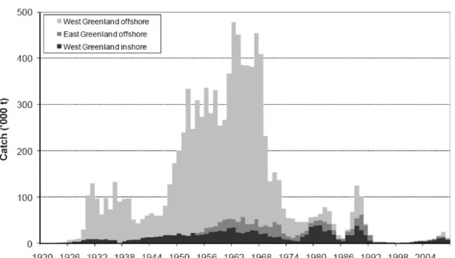
1.1 Atlantic cod landings in Greenlandic waters since 1920, divided in the three different stocks from this area (ICES Advice Book 2 2009) . . . 2 1.2 Female Atlantic cod (Gadus morhua) caught along the East Greenland coast in

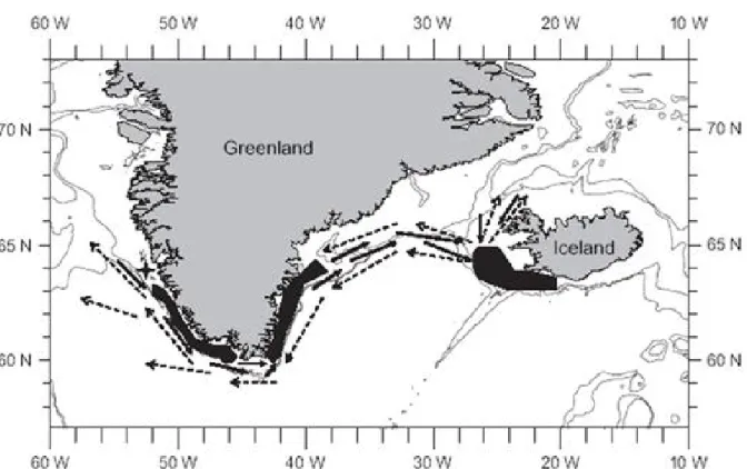
autumn 2017 . . . 3 1.3 Migrations patterns of Atlantic cod around Greenland. Dashed arrows are

indicating larval drifts with the Irminger, East Greenland and West Greenland Current. Black arrows are indicating homing migration of adult cod. (Rätz et al.

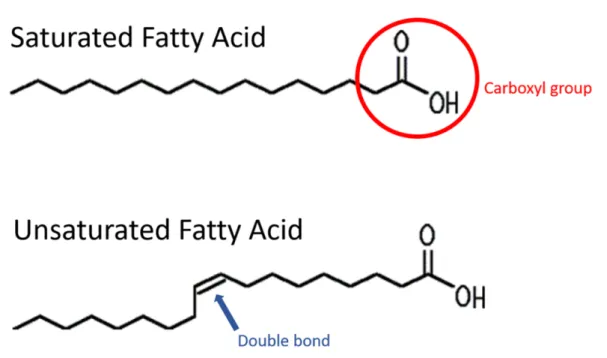
2005) . . . 4 1.4 Schematic of the chemical structure of fatty acids. On top a saturated fatty acid

(SFA) with no double bond, the carboxyl group is indicated by the red circle. At the bottom a mono unsaturated fatty acid (MUFA) with a cis double bond . . . 5 2.1 Schematic Greenland current systems, sampling stations and sites. Solid lines

show observed paths of the East Greenland current (EGC), East Greenland coastal current (EGCC), and the Irminger current (IC), while dashed lines indi- cate possible flow paths induced by bathymetric or wind effects. WGC= West Greenland Current. Adapted from Sutherland and Pickart (2008) . . . 10 2.2 Deploying the BT140 (bottom trawl) net in Greenland autumn 2017 . . . 11 2.3 Liver tissue index 0. Liver tissue is totally solid . . . 15 2.4 Liver tissue index 1 (left) and liver tissue index 2 (right). Liver tissue index 1

still has large solid parts (right site) and only little degradation (middle). Liver tissue index 2 only has small solid parts left (lower part of the liver) the rest is mainly fluid and only held together by the outer membrane of the liver. This liver also shows a high macro parasite loading . . . 15 2.5 Liver tissue index 3. No solid tissue parts are left. Full degradation of the tissue.

Yellow circle at the right picture indicates an ulceration with encapsulated parasites 15 3.1 Total lipid contents of gonads (left) and livers (right). On the x axis are the three

sampling sites. The y axis shows the fat content in percent of dry weight . . . . 21

3.2 Box and whisker plot of the mount of the most important gonad fatty acids and fatty acid groups in ng/mg dry weight. The three sampling sites are dis- played on the x axis. The y axis shows fatty acid amounts in ng/mg dry weight.

Arachidonic acid (ARA), Eicosapentaenoic acid (EPA), Docosahexaenoic acid (DHA), saturated fatty acids (SFA), mono unsaturated fatty acids (MUFA), poly unsaturated fatty acids (PUFA), total fatty acids (TFA) . . . 22 3.3 Box and whisker plot of the percentage contribution of the most important gonad

fatty acids and fatty acid groups to total fatty acids (TFA). The three sampling sites are displayed on the x axis. The y axis shows fatty acid contribution in per- cent of total fatty acids. Arachidonic acid (ARA), Eicosapentaenoic acid (EPA), Docosahexaenoic acid (DHA), saturated fatty acids (SFA), mono unsaturated fatty acids (MUFA), poly unsaturated fatty acids (PUFA) . . . 23 3.4 6 Liver macro parasites from an individual of site 1 (left) and an individual of

site 3 (right) . . . 25 3.5 Prey indices for every individual fish and site. Colours indicate the main prey

origin . . . 26 3.6 Species contribution (%) to the total stomach content weight of each individual.

Unidentifiable, highly digested matter is combined as other remains. The Taxon Molluscs contains mainly Bivalvs, Gastropods and in some cases Theutids. Hard matter like stones and sand were combined as benthic remains. Colours and prey species are sorted by prey origin, pelagic on top, benthic on the bottom . . . 27 3.7 Stable isotope ratios of 30 fish, data for fish 4 and 7 were not available. On the x

axisδC13 and on the y axisδN15. Sites are indicated by colour. a. is showing mean ratios of the sites, the error bars are showing the standard deviation. b.

is showing the stable isotope signature for each individual. Numbers resemble FishID . . . 28 3.8 Scree stack plot of the principal component analysis (PCA). The x axis shows

the dimensions and the y axis shows the percentage of explained variance . . . 30 3.9 Principal component analysis of all parameters with data from 30 individual

fish. Fish 4 and 7 are missing, due to a lack of stable isotope data. On the x axis dimension 1 and the percentage contribution of the dimension to the explained variance. On the y axis dimension 2 and the percentage contribution of the dimension to the explained variance. The single data points resemble the individual fish, colours indicate the sampling site. The vectors show the explanatory variables and their correlation between each other and the dimensions 31 3.10 Redundancy analysis (RDA) for explanatory variables that were chosen by a

prior SIMPER analysis and all fatty acids . . . 32

List of Figures List of Figures

3.11 Redundancy analysis (RDA) for explanatory variables that were shosen by a prior SIMPER analysis and all fatty acid groups plus the Eicosapentaenoic acid (EPA) to Arachidonic acid (ARA) ratio . . . 33

List of Tables

2.1 Criteria to determine the liver tissue degradation . . . 14 2.2 Criteria to determine the degree of filling of stomachs . . . 16 2.3 Criteria to determine the digestion rate of prey species dissected from stomachs 16 2.4 Prey categories to determine prey origin and prey index . . . 17 3.1 Condition indices and fish parameters. Mean Hepatosomatic index (HSI), Go-

nadosomatic index (GSI), condition factor K, length in centimeters, age in years and weight in grams per site are listed with standard deviation. (Site 1 n= 12;

Site 2 n= 10; Site 3 n= 10) . . . 24 3.2 Mean parasite indices and liver tissue indices per site are listed with standard

deviation (Site 1 n= 12; Site 2 n= 10; Site 3 n= 10) . . . 25 3.3 Mean Shannon index of stomach contents per site and mean prey indices per site

are listed with standard deviation. (Site 1 n= 12; Site 2 n= 10; Site 3 n= 10) . . 27 3.4 Sampling sites and station properties. All sites with their sampling stations and

number of sampled individuals are shown. Mean depth, sea surface temperature (SST) in degrees Celsius, bottom temperature (BT) in degrees Celsius, sea surface salinity (SSS) in practical salinity units (PSU) and bottom salinity (BS) in PSU are listed . . . 29 5.1 Output Kuskar-Wallis Test; Site 1 n=12, Site 2 n=10, Site 3 n=10 . . . 51 5.2 Output Kuskar-Wallis Test; Site 1 n=12, Site 2 n=10, Site 3 n=10 . . . 52

List of Tables List of Tables

Glossary

ARA Arachidonic acid

BS Bottom salinity

BT Bottom temperature

δC δC Stable Isotope ratio of 13C to 12C

DHA Docosahexaenoic acid

δN δN Stable Isotope ratio of 15N to 14N

EGC East Greenland Current

EGCC East Greenland Coastal Current

EPA Eicosapentaenoic acid

GSI Gonadosomatic index

HSI Hepatosomatic index

IC Irminger Current

K Fish condition factor

MUFA Mono unsaturated fatty acids

ParaIndex Parasite index

PUFA Poly unsaturated fatty acids

SFA Saturated fatty acids

SSSal Sea surface salinity

SST Sea surface temperature

SWInd Shannon-Wiener Index of stomach content

TFA Total fatty acids in ng/mg dry weight

TFGonads Total lipid content of gonads

TFLiver Total lipid content of liver

1

Introduction

1.1 Motivation

The cod stocks in Greenland waters once were among the largest in the world (Sundby 2000).

Landings increased in the early 20th century and peaked in the 1960s with a catch size of up to 460,000 t per year (Figure 1.1). In the early 1970s, the off-shore stocks collapsed due to a combination of high fishing pressure and a decrease in temperature (Buch et al. 1994) and could never recover completely. Even though the collapse was severe and Greenland’s economy is largely dependent on fisheries (Hamilton et al. 2003), there is still little known about food web interactions and the impact of oceanography on condition of Atlantic cod in Greenland waters.

Timeseries data of condition and stomach content analysis revealed distinctive patterns of cod condition and prey preferences along the East Greenland coast (Werner et al. 2018) that were consistent over time and might be influenced by the oceanography and environmental features in these areas. So far there are no studies from this area, which specializes on large, mature female fish, which have a prominent role when it comes to reproduction and resilience of stocks (Marteinsdóttir & Steinarsson 1998; Scott et al. 1999; Berkley et al. 2004; Hixon et al. 2013).

Additionally, there are no studies using methods like fatty acid profiles and stable isotopes of cod in Greenland waters that give an idea about larger time scale food web interactions, compared to stomach content analysis. Fatty acid profiles have the potential not only to give insight into food web interactions but also into food quality, temperature adaption, condition and the reproductive outcome of an individual (Dalsgaard et al. 2003, Tocher et al. 2003, Arts and Micheal T. 257-280 in Lipids in Aquatic Ecosystems 2009, Røjbek et al. 2014). Together with fatty acid analysis, stomach contents and stable isotopes provide an intresting tool to link oceanography, food web interactions and fish physiology like condition and reproductive outcome.

Figure 1.1: Atlantic cod landings in Greenlandic waters since 1920, divided in the three different stocks from this area (ICES Advice Book 2 2009)

1.2 Atlantic cod in Greenland waters

Atlantic cod (Gadus morhua) (Picture 1.2) is a widely dispersed demersal fish species in the North Atlantic where it is ecologically and economically highly important (Ottersen et al. 2006) and therefore of great interest in several research fields. Since the cold arctic waters represent the northern-most distribution range of this species (Hansen 1949, Buch et al. 1994), growth, recruitment and the productivity of the populations here do strongly depend on temperature (Rätz et al. 1999, 2003, 2005; Brander et al. 1995). The oldest reports of Atlantic cod in the waters around Greenland date back to the 16th century and its occurrence and abundance underwent large natural fluctuations since then (Schmidt 1931). From the late 1920s on fishing became an additional driver for changes in numbers (Figure 1.1). Today, cod in Greenland waters are thought to consist of three different stocks. Two offshore stocks in East and West Greenland and the inshore stock in the large and distinct fjord systems along the west coast (ICES 2018).

Introduction 3

Picture 1.2:Female Atlantic cod (Gadus morhua) caught along the East Greenland coast in autumn 2017

All stocks show different migratory behavior (Figure 1.3) but at least for the offshore stocks similar egg drift patterns. In some irregularly occurring years of high recruitment in the waters around Iceland, there is also an influence of recruits from Iceland stocks (Begg et al. 2000, Wieland et al. 2002).

Eggs and larvae from East Greenland and Iceland stocks are drifting with the East Greenland current (Figure 2.1) from the spawning grounds in East Greenland and Iceland south-westwards, along the coast to West Greenland where they settle on offshore banks and migrate back as soon as they become mature (Rätz et al. 2005, Bonanomi et al. 2016, ICES 2018). The majority of individuals from stocks in the fjord systems are however sedentary (Hansen 1949, Storr-Paulsen et al. 2004). The stock on West Greenland offshore banks is nowadays comparably small (ICES 2018) and specimens are migrating along the West Greenland coast (Storr-Paulsen et al. 2004), causing a distinct age pattern along the coast of the island, with a larger proportion of older and better conditioned specimens in East Greenland and younger ones in south-west Greenlandic waters (ICES 2015). As a regional effect, cod in the waters around Greenland is in general (with some exceptions) of less good condition compared to more southerly populations (Rätz et al.

2003) and is showing an enhanced fluctuated recruitment. Since the arctic waters represent its northern-most range of distribution (Hansen et al. 1949, Buch et al. 1994), these effects are partly temperature dependent (Rätz et al. 1999; Ottersen et al. 2006).

Figure 1.3: Migrations patterns of Atlantic cod around Greenland. Dashed arrows are indicating larval drifts with the Irminger, East Greenland and West Greenland Current. Black arrows are indicating homing migration of adult cod. (Rätz et al. 2005)

1.3 Lipids and fatty acids

The major role of lipids in fish is the storage of metabolic energy in form of ATP, that is provided byβ-oxidation in mitochondria (Sargent et al. 1989, Froyland et al. 2000). One of the constituents in lipids are fatty acids. Fatty acids play an important role in every living organism from bacteria to plants to metazoans and hence fish. They are ubiquitous and involved in many main functional and structural traits of live, like cell membranes, energy storage (Tocher et al. 2003) and hormone production (Johnston et al. 1985). In fish they are the preferred source of metabolic energy used for growth, movement and therefore migration and reproduction (Tocher et al. 2003). Fatty acids mainly consist of a carbon chain that is either saturated (Saturated Fatty Acids = SFAs) and containing no double bonds or unsaturated containing one (Mono Unsaturated Fatty Acids = MUFAs) or more double bonds (Poly Unsaturated Fatty Acids = PUFAs and Highly Unsaturated Fatty Acids = HUFAs) plus a carboxyl group (Figure 1.4) (Tocher et al. 2003).

Introduction 5

Figure 1.4: Schematic of the chemical structure of fatty acids. On top a saturated fatty acid (SFA) with no double bond, the carboxyl group is indicated by the red circle. At the bottom a mono unsaturated fatty acid (MUFA) with a cis double bond

Most natural fatty acids have an even number of carbon atoms and their structure and function e.g. the melting point, depend on the length of the carbon chain, the number and kind of double bonds (cis or trans) and their position within the carbon chain (Tocher et al. 2003). The predominant SFAs occurring in animal lipids are C16:0 and C18:0, they can be produced de novo by every animal (Sargent et al. 1989). The predominant MUFAs in lipids are C18:1n-9 and C16:1n-7. Whereas fish lipids, especially in high latitudes are also very rich in 20:1n-9 and 22:1n-11, originating from zooplanktonic wax esters from mainly calanoid copepod species (Sargent and Henderson, 1995). In fish the main PUFAs are Arachidonic acid (20:4n-6) and its precursor Linoleic acid (18:2n-6) and Eicosapentaenoic acid (20:5n-3) and Docosahexaenoic acid (22:6n-3) and their precursor Linolenic acid (18:3n-3). These precursors are essential fatty acids for all vertebrates and therefore fish, and can later on be elongated and desaturated to the PUFAs mentioned before (Tocher et al. 2003). This means that fish including cod are incapable of producing these PUFAsde novo. Cod liver is in general very rich in these PUFAs and therefore widely used to produce dietary supplements in form of fish oil capsules for humans. PUFAs have a crucial role for organisms. They are important structural parts of the cell membrane and therefore involved in cell communication and transport of matter as well as in the maintenance of membrane fluidity (Singer and Nicolson 1972) under changing temperatures (Farkas et al. 1981, Arts and Michael 2009). A subset of these PUFAs, the eicosanoids can act as precursors for hormones involved in several pathways including reproduction (Johnston et al. 1985; Dalsgaard

et al. 2003). Since marine food webs are rich in lipids unlike freshwater systems, these PUFAs are usually obtained directly from the food source instead of being anabolized from their precursors (Tocher et al. 2003). High lipid amounts in food are even suppressing a de novo fatty acid production (e.g. Shimeno et al. 1995 and 1996). By this mechanism the fatty acids are channeled up the food web (Dalsgaard et al. 2003). Depending on the group of phytoplankton dominating the first trophic level of the food web and also depending on environmental influences, fatty acid composition can vary significantly between individuals and areas (Dalsgaard et al. 2003). In the marine realm latitudinal differences in fatty acid profiles of copepod species were already found (Kattner and Hagen 2009). Additionally, climate and climate change can have an impact on plankton community composition and their fatty acid profiles (Dalsgaard et al. 2003, Kattner and Hagen 2009). Therefore, regional influences, like food sources and abiotic factors might also be manifested in the fatty acid profiles of cod in Greenland waters.

1.4 Importance of female fish condition and its linkage to lipid compositions

A keystone for the recovery of fish stocks is the spawning stock biomass, its age structure and the reproductive outcome of the individual fish, as well as the general condition (Kjesbu et al.

1991; Marteinsdóttir & Steinarsson, 1998; Berkley et al. 2004; Hixon et al. 2013; Rätz et al.

2002; Ottersen et al. 2006). Especially females and their condition have an important role for the survival of the offspring (Marteinsdóttir & Steinarsson, 1998; Scott et al. 1999). It is widely known that larger and older females (BOFFFFs) have the highest egg qualities and egg quantities (Berkley et al 2004; Hixon et al. 2013). Their spawning times are extended and batch numbers are higher compared to younger and more unexperienced individuals (Hixon et al. 2013). This is causing a higher survival and therefore larger contribution of offspring to recruitment from older females, due to an enhanced chance of matching spawning times with good environmental conditions (Hedgecock 1994). Hence maternal effects are of great importance for the health of fish stocks (Marteinsdóttir & Steinarsson, 1998) and the evaluation of longterm consequences of fisheries, as they have the potential to buffer extreme environmental fluctuations (Hixon et al.

2013). General condition, energy storage and resource allocation can be considered as some of these maternal effects. Cod is a lean fish, meaning the fat storage is basically located in the liver instead of muscles or around inner organs (Lambert & Dutil 1997b). These liver fat storages are then allocated to the gonads before spawning, causing a negative correlation of Hepatospmatic index (HSI) to Gonadosomatic index (GSI) (Røjbek et al. 2012). Especially the fatty acid composition of this fat storages, that is driven by the diet of the individuals (Dalsgaard et al 2003, Tocher et al. 2003, Røjbek et al. 2014), can later have an influence on the quality

Introduction 7

of the offspring (Sargent et al. 1999). Røjbek et al. (2012, 2014) found a correlation between the ratios of important PUFAs Arachidonic acid, Eicosapentaenoic acid and Docosahexaenoic acid with the fecundity, the hatching success and survival of the larvae and the maturity stage of female cod. Whereas a total reduction of the fat content can force females to skip spawning in certain seasons (Rideout et al. 2006) and is related to a reduction in hormones that are involved in the gonadal development (Cerdá et al. 1994, Matsuyama et al. 1994). A shift in the diet and hence the fatty acid composition of Atlantic cod in the Baltic Sea was correlated with a shift in maturity and spawning times (Tomkiewicz et al. 2010) which can lead to a miss match between spawning times and environmental conditions suitable for the development of eggs and larvae.

1.5 Feeding patterns and stable isotopes

Different habitats in the marine realm are dictated by different abiotic and biotic environmental factors, such as current systems, temperature and salinity gradients or varying depth profiles, as well as predators or competitors, parasites, prey abundance and composition. In Greenland waters, cod feeds in pelagic and benthic habitats. Its most important prey species are capelin (Mallotus villosus), krill (Meganyctiphanes norvegica), benthic crabs (Majidae), redfish (Sebastes sp.), mesopelagic fish, amphipods (Hyperiidae and Gammaridae) and northern shrimp (Pandalus borealis) (Nielsen & Andersen 2001, Hedeholm et al. 2016, Werner et al. 2018). Importantly, diet composition is a strong predictor of condition, energy storage and lipid content in cod (Lie et al. 1988, Jobling 1988). While stomach content analysis show short-term feeding patterns, stable isotopes contain information about diet preferences weeks to month prior to sampling (Hobson 1999). Hence, stable isotope analysis can be used to examine food web interactions and trophodynamics. Stable isotope signatures are dependent of the source of isotopes (e.g.

terrestrial or marine) and their fractionation (Peterson and Fry 1987). Most often Carbon and Nitrogen isotopes are used for this purpose. The mean fractionation from one trophic level to the next is about 3.4hforδ15N and 0.4hforδ13C (Post 2002). Carbon isotopes can also be used to determine benthic or pelagic food sources (Dunton 1989, Hobson 1994, Agurto 2007).

By setting a source baseline, which is in marine pelagic systems preferably phytoplankton, and adding the information about fractionation of nitrogen isotopes, trophic levels of individuals can be determined (Post 2002) and a food web can be reconstructed. Since the isotope signature is shaped by a diversity of biogeochemical processes which differ between regions, stable isotope analysis can also be used to examine migration patterns and link individuals to a certain area they formerly occupied (Hobson 1999). For this study an isotope baseline is missing, which limits the explanatory power of the analysis. Nevertheless, the signatures are still able to display differences between fish, which are generated by different diets and different biogeochemical processes, in each habitat.

1.6 Oceanography

The fatty acid composition of an individual is largely influenced by its diet composition (Dalsgaard et al. 2003, Tocher et al. 2003; Jobling & Leknes 2010, Røjbek et al. 2014) and can as well as the general condition be influenced by the environment, hence the habitat or region that it lives in (Sargent and Henderson 1995). The samples for this study were collected from different habitats along the east and south-west coast of Greenland, separated by distance and climate regimes as well as current systems and differing in their depth profiles (Figure 2.1, Table 3.4).

Sample collection started on the Dhorn Bank with sampling site 1 (Figure 2.1). The northern most sampling station is mainly of arctic influence. The mixture between the warmer and saltier Irminger Current and the East Greenland Current (Rudels et al. 2002) is providing high production and food abundance in this area. The short distance to the continental slope, plus the influence of the Irminger Current are linking sampling site 1 to the mesopelagic food web.

Following the low saline and cold East Greenland Current southwards reaching Kleine Bank at sampling site 2 (Buch 2002), where samples were taken within a resident eddy system between the east Greenland current (EGC) and the east Greenland coastal current (EGCC) (Figure 2.1).

The primary production in this area seems to be decoupled from the surrounding area with an earlier peak in spring blooms and inter annual changes in zooplankton communities (Fock et al unpublished, Stippkugel 2018). Ending at the southern tip of Greenland at sampling site 3, around the corner of Cape Farwell that is dominated by warmer North Atlantic waters (Buch et al. 1994), keeping this region mainly ice free and representing subarctic conditions (Buch 1990,2000) and also having the shallowest sampling depth (Table 3.4).

1.7 Importance and research objectives

Habitat can have a a strong influence on the condition (Pardoe et al. 2008) and reproduction of fish (Kjesbu et al. 1991), especially at the extremities of their distribution ranges, where recruitment success can be highly sensitive to environmental fluctuations (Berkley et al. 2004).

This sensitivity towards extreme environmental fluctuations is even more enhanced in populations, which experience high fishing pressure, that is disturbing the age structure in spawning stock biomass (Berkley et al. 2004). Well-conditioned females can positively influence the buffering capacity towards environmental fluctuations and hence increase the recruitment success in these environments (Ottersen et al. 2006, Hixon et al. 2013). Regional effects on the condition and reproductive outcome of female Atlantic cod should therefore be considered in stock management, since the populations in Greenland waters still show a lack of resilience and could never recover from the severe collapse in the late 20th century (ICES 2018a).

Introduction 9

The different regional influences of oceanographical and biological origin in the waters around Greenland, indicate the existence of regional differences in food abundance and feeding behavior (benthos vs. pelagic). This is causing differences in the general condition of cod (Werner et al.

2018) and will probably also cause differences in its total lipid content as well as differences in the fatty acid composition of the individuals and hence differences in the reproductive outcome of cod in Greenland (Røjbek et al 2014). In order to reveal the existence of regional differences in condition and reproduction of female Atlantic cod in Greenland waters, that has been and still is suffering from high fishing pressures, this study will investigate potential differences in feeding preferences by looking mainly at total lipid contents of livers and ovaries as well as the fatty acid composition of the later and different ratios in stable isotope enrichments.

Methods

2.1 Sampling

Samples were collected during the annual German Bottom Trawl Survey in Greenland with the FFS Walther Herwig III of the Thünen Institute for Sea Fisheries from 06.10.2017 to 17.11.2017 (WH410). Three different sites in East and South Greenland were sampled (Figure 2.1, Table 3.4).

Figure 2.1: Schematic Greenland current systems, sampling stations and sites. Solid lines show observed paths of the East Greenland current (EGC), East Greenland coastal current (EGCC), and the Irminger current (IC), while dashed lines indicate possible flow paths induced by bathymetric or wind effects. WGC= West Greenland Current. Adapted from Sutherland and Pickart (2008)

In order to collect only mature female cod, a size range of 75-90cm was chosen. At least 10 specimens were sampled per site. A survey bottom trawl net (BT140 bobbin gear) (Picture 2.2) with pony otter boards and a cod end mesh size of 20mm was used to collect the samples (Supplementary).

Methods 11

Picture 2.2:Deploying the BT140 (bottom trawl) net in Greenland autumn 2017

Right after the catch, fish were slaughtered and total, gutted, gonad and liver weight, as well as total length were collected as part of the biological sampling protocol on board. The otoliths were dissected from the head and kept in paper bags for age determination. Stomachs were dissected from the abdominal cavity and stored in plastic bags kept on ice, until final freezing at minus 30^◦C. The gonads and livers were kept on ice until the final tissue sampling for total lipid content and fatty acid composition could be done. Gonad tissue was always sampled from the right lobe, even though ovaries of Atlantic cod are presumed to be homogenous (Witthames et al. 2009). Liver tissue was always sampled from the smallest lobe, after carefully removing the macro liver parasites, to make sure only pure liver tissue was sampled. The tissue samples were collected then in 2.5 ml cryo-tubes and stored in liquid nitrogen (-196^◦C). Tissue samples for stable isotopes were taken from the left side of the dorsal muscle behind the head and kept in cryo-tubes at minus 30^◦C.

2.2 Lipids and fatty acids

2.2.1 Total lipid content of livers and gonads

The extraction of lipids was done by a modified version of the methods described in Bligh and Dyer (1959) and Folch and colleagues (1956). Subsamples of liver and gonad tissue were freeze dried for at least 24 hours in a Christ Alpha 1-2 LDplus freeze-dryer, with a condenser temperature around -63^◦C and a pressure of about 0.36 mbar. Afterwards the tissue was extracted three times for 24h at -20^◦C, using a 1:1:1 Chloroform/ Dichloromethane/ Methanol (CHCL3/

CH2CL2/ CH3OH) extraction mix. The total fat content was then determined gravimetrically by subtracting the weight of the extracted tissue from the tissues dry weight.

2.2.2 FAME (Fatty Acid Methyl Ester) analysis

The extraction of lipids was done by a modified version of the methods described in Bligh and Dyer (1959) and Folch and colleagues (1956). By using this method, all fatty acids from all lipid fractions are extracted and after using the following steps esterified and quantified. A supplementary assignment to the lipid fractions is not possible and would need prior separation of the lipid extract in silica columns. Fatty acid methyl esters were measured for gonad tissue samples.

Extraction and internal-standard additions

Wet weights of all gonad tissue subsamples were taken. Subsequently the tissue samples were freeze dried for about 24 hours in a Christ Alpha 1-2 LDplus freeze-dryer, with a condenser temperature around -63^◦C and a pressure of about 0.36mbar. Gonad samples were afterwards grinded to a powder by using a mortar. Dried sub samples were weight into glass vials and the lipids were extracted with an addition of 3 ml CHCL3/ CH2CL2/ CH3OH Chloro- form/Dichloromethane/Methanol (1:1:1) for at least 12 hours at -20^◦C. 100µL of C19:0 FAME (c=22.03_µL^ng) and C21:0 (c=30.08_µL^ng and 30.09 _µL^ng) as a fatty acid were added as internal standards.

Clean up

The extracted lipids were transferred to a separation funnel and the glass vials were spilled 2 times with 2 ml of the CHCL3/ CH2CL2/ CH3OH (1:1:1) solvent mixture. The chloroform layer was then separated by adding 2.25ml of 1M KCL solution. The lower layer was kept in a conical flask. The upper layer was rinsed 2 times with dichlormethane. NaSO4 was added to the conical flasks to avoid any water in the extract. Afterwards the extract was transferred to a centrifuge tube (2 times of re-extraction with 1.5ml dichlormethane).

Methods 13

Evaporation and pre-preparation

The extract was cooled down for one hour at -20^◦C. Subsequently the extract was reduced to total dryness in a rotary film evaporator (Heidolph Laborota 4000 efficient). The extract was re-dissolved with 100µL Chlorofrom (CHCL3) and transferred into a glass cocoon (Two times of rinsing the centrifuge tubes with 100µL CHCL3). Finally, the solvent was again removed by using the rotary film evaporator.

Esterification

After evaporation 100 µL of Toluene and 200 µL of 1% H2SO4 in CH3OH (50 ml CH3OH + 0.233µl of concentrated H2SO4; 97%) was added to the cocoon. Afterwards the co- coon was flushed with N2, closed and heated up to 50^◦C for at least 12 hours by using a sand bath.

Re-extraction and analyses

After an addition of 300µL of 5% sodium chloride solution (2.5 g NaCl in 47.5g Milli-Q water) the esters were then extracted in 3 portions of 100µL n-hexane into a new glass cocoon. The solvent was reduced until dryness by using the rotary film evaporator again. The extract was re-dissolved with n-hexane to a final volume of 100µL. 1µl of the final extract was analyzed by using a fast gas-phase chromatograph (Thermo ELECTRON CORPORATION Trace GC Ultra) coupled with an autoanalyzer (Thermo SCIENTIFIC AS 3000). The injection was splitless on a capillary column and hydrogen was used as carrier gas. An external standard of Supelco^R 37 Component FAME Mix (supplementary) with a concentration of 40ng C19 per 1µl and a Bacterial Acid Methyl Ester (BAME) Mix (supplementary) were run three times and once before every set of analysis. Peak identification was done by retention times, comparing the external standard to the actual sample. Concentrations of fatty acids were afterwards calculated based on the peak area of the C19:0 internal standard. The internal C21:0 standard was used to check for the quality of esterification. For statistical analysis and plotting of data, the total quantities of fatty acids in Nanograms were chosen, to gain an overview about the actual energy storage and resource stocks of the gonads. Together with the percentage values depletions or enrichments in certain fatty acids or fatty acid groups can be determined.

2.3 Condition factors and liver health

2.3.1 Condition factors

Because gadoid fish species (Lloret, Shulman & Love, 2013), such as cod, store largest parts of their energy in the liver, the hepatosomatic index (HSI) as percentage contribution of liver weight to gutted fish weight, was chosen as main index of condition and energy storage (Lambert

& Dutil 1997b). Furthermore, HSI is more sensitive to diet variability and can better reflect spatial differences of diet (Jobling et al. 2010, Pardoe et al. 2008). The morphometric condition factor K, Hepatosomatic index (HSI) and Gonadosomatic index (GSI) were calculated for each individual using the following equations:

K =

HSI (Hepatosomaticindex) =

guttedweight

∗ 100

GSI (Gonadosomaticindex) =

guttedweight

∗ 100

2.3.2 Liver parasites and tissue

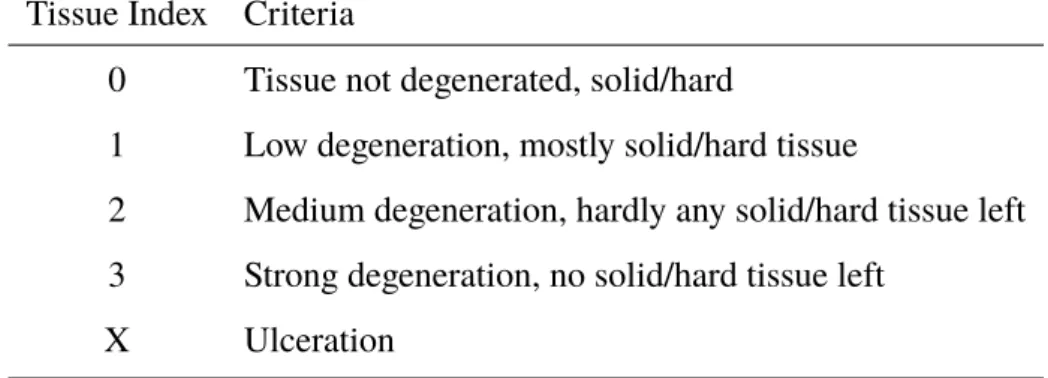
During sampling and parasite dissection, differences between the consistence of liver tissues were recognized. These differences might affect liver physiology and therefore, a liver tissue index was developed to document these differences. In the laboratory livers were defrosted in a warm water bath. The index was determined by using the following criteria (Table 2.1, Picture 3.3, Picture 3.4, Picture 3.5), before dissecting all parasites from the tissue.

Table 2.1:Criteria to determine the liver tissue degradation Tissue Index Criteria

0 Tissue not degenerated, solid/hard

1 Low degeneration, mostly solid/hard tissue

2 Medium degeneration, hardly any solid/hard tissue left 3 Strong degeneration, no solid/hard tissue left

X Ulceration

After determination of the liver tissue index, all macro liver parasites (Picture 4.4) were dissected carefully with forceps and weighted. The Parasite index represents the percentage contri- bution of liver macro parasites to liver weight and was calculated by using the following equation:

P arasiteIndex =

Liverweight

∗ 100

Methods 15

Picture 2.3:Liver tissue index 0. Liver tissue is totally solid

Picture 2.4:Liver tissue index 1 (left) and liver tissue index 2 (right). Liver tissue index 1 still has large solid parts (right site) and only little degradation (middle). Liver tissue index 2 only has small solid parts left (lower part of the liver) the rest is mainly fluid and only held together by the outer membrane of the liver. This liver also shows a high macro parasite loading

Picture 2.5: Liver tissue index 3. No solid tissue parts are left. Full degradation of the tissue. Yellow circle at the right picture indicates an ulceration with encapsulated parasites

2.4 Feeding patterns and stable isotopes

Stomach content analyses were made, in order to gain an overview of the feeding preferences of the individual fish of different habitats. The stomachs were defrosted in a warm water bath.

Full stomach and empty stomach weights were taken before the content analysis. The stomachs were cut open by using scissors. The content was then sorted and the ingested organisms were if possible, identified down to species level, counted and weight. Fish prey was identified by their otoliths, using the Otolith Atlas by Campana (2004) and our own reference collection.

Invertebrates were identified by using the following literature (Schneppenheim & Weigmann- Haass 1986; Baker et al. 1990; Hayward & Ryland 1990a, b). Digestion rates and filling degree were determined using the following categories (Table 2.2, Table 2.3):

Table 2.2:Criteria to determine the degree of filling of stomachs Filling Degree Criteria

0 Stomach is empty, stomach wall is thick, distinct gastric rugaes 1 Stomach is partly filled, stomach wall is thick, distinct gastric rugaes

2 Stomach is filled, stomach wall is thinner, some parts smooth with no rugaes 3 Stomach is fully filled, stomach wall is thin, no gastric rugaes

Table 2.3: Criteria to determine the digestion rate of prey species dissected from stomachs Digestion Rate Criteria

1 No signs of digestion, net feeding 2 Small signs of digestion

3 Medium signs of digestion

4 Strong digestion, organism is only identifiable by special features left (e.g. otoliths) 5 Full digestion, organism is not identifiable anymore

Methods 17

Table 2.4: Prey categories to determine prey origin and prey index Prey Categories Prey Orignin

1 Benthic

2 Unkown

3 Pelagic

A Prey Index was calculated by using the following prey categories and equation to determine differences in the food preferences of each fish (Table 2.4):

P reyIndex =

The closer the prey index is to the value of a prey category the more the individual was preying on prey from this certain category. To determine differences in the diversity of the prey, the Shannon-Index, which takes into account both the number of species and its proportion, was calculated for each stomach by using the following equation:

H ⁰ = P _S

i=1 p _i lnp _i

H⁰ =diversity p_i =weightof eachspecies

S =numberof species

In addition to the stomach content analysis, which reflect short term diet patterns, stable isotope analyses were performed to have a better understanding of the trophic interactions and long-term feeding preferences of the fish. Therefore, the muscle tissue was freeze dried for at least 12 hours in a Christ Alpha 1-2 LDplus freeze-dryer, with a condenser temperature around -63^◦C and a pressure of about 0.36mbar. Afterwards tissue was grinded to a fine powder by using a mortar. Tissue powder was weighted in tin capsules (3.2x4mm, HEKAtech GmbH, Wegberg/Germany), using a Sartorius micro-balance with a resolution of 10-4mg. A sample amount of 0.04-0.06mg was used for analysis (Hansen et al. 2009). Between every step all tools were cleaned by using fuzz free cleaning tissues and Acetone. The analysis was done by a high sensitivity elemental analyzer (CE INSTRUMENTS EA1110) coupled with an isotope mass spectrometer (DeltaPlus Advantage, Thermo Fisher Scientific). Acetanilide (C8H9NO) was

used as internal standard and measured in between samples to calibrate the measurements. The ratios were calculated by the following equation (Hansen et al. 2009):

δX = ( _Rstandard ^Rsample - 1) * 1000

X =δ15N orδ13C R = 15N:14N or 13C:12C

2.5 Oceanography

All hydrographic data were collected using a CTD probe (Seabird 911+ carousel). Not all of the fishing stations had actual CTD data. Therefore, data from the closest CTD station was chosen by using the following distance equation:

Distance= 2∗6371000∗arcsin r

sin(LAT2∗π

180 )−(LAT1∗ ₁₈₀^π 2 )²+ r

cos(LAT2∗π

180 )∗cos(LAT1∗π

180 )∗ sin(LON G2∗π

180 )−(LON G1∗ ₁₈₀^π

2 )²

LAT1 = Latitude sampling station LAT2 = Latitude corresponding station

LONG1 = Longitude sampling station LONG2 = Longitude corresponding station

2.6 Statistical analysis

All statistical analysis was done with R version 3.3.1 (2016-06-21)(R Development Core Team (2008)). Data selection was done using the dplyr package (Wickham et al. 2017). Statistical analysis was divided in a univariate and a multivariate part. For the univariate part all measured variables were tested separately for significant differences between the sites by using two non- parametric tests. Fatty acids were tested as individuals and once in groups (SFAs, MUFAs, PUFAs, TFAs). A Kruskal-Wallis test was done for every variable to check for general significant differences between the sites. All variables that were significantly different in the Kruskal-Wallis

Methods 19

testing were then subsequently analyzed by using a post hoc pairwise Wilcoxon-rank-sum test, that revealed which sites were significantly different from each other. As the first part of the multivariate statistical analysis a PCA (Principal Component Analysis) was used to visualize the existing differences between the sampling sites and to determine the main drivers for differences.

Therefore, all measured fatty acids and fatty acid groups plus the explanatory variables for site were used as variables in this PCA. To know which of these variables to prefer for the PCA a similarity percentage (SIMPER) analysis was done initially using the vegan package (Oksanen et al. 2018). The SIMPER function performs pairwise comparisons of groups of sampling units and finds the average contributions of each species to the average overall Bray-Curtis dissimilarity. The PCA was done by using the R packages FactoMineR (Le et al. 2008) and factoextra (Kassambara et al. 2017) and interpreted by using the following biplot-rule adapted from Leyer & Wesche (2007). A PCA is using a similarity matrix of variables based on the Pearson correlation coefficient, to extract an axis, here called dimension, that is explaining the most variance in the data. The second axis or dimension is then generated by the maximum amount of variance left and is orthogonal to the first axis or dimension. This continues until all variance is represented in a dimension. The less dimensions it takes to explain the most variance in the data, the better. The variables itself are represented as vectors, originating from the middle of the newly formed coordinate plane. On the basis of their length and position to each other and to the dimensions, the correlation between the variables itself and between the variables and the axis can be displayed. The correlations between variables and axes is additionally described by loadings. They reach from +1 to -1 and equal therefore the Pearson correlation coefficient. If a variable has a high loading on one axis or dimension, it increases (if it is a positive loading) or decreases (if it is a negative loading) strongly with this axis. The correlations among the variables can in simple words be displayed by the angle Îś in which they are position to each other.

An angle below 90^◦is a positive correlation, an angle of 90^◦corresponds with no correlation at all and above 90^◦is a negative correlation. To integrate the samples, in this case the individual fish, in this coordinate plane, every value of the variable for each sample is multiplied by the axis loading of the variable. These products are then summed up for every variable and transferred as a coordinate into the plane. As a second step of the multivariate statistical analysis, two Redundancy Analysis (RDA) were done, using the vegan package (Oksanen et al. 2018) in R. For the first RDA model the fatty acid composition in nanograms was used as the response matrix.

For the second RDA model fatty acid groups were used. Explanatory variables were chosen using a SIMPER analysis of all condition indices, hydrographical data and all other parameters e.g. liver macro parasites and stable isotope analysis, that were taken and significant in the Kruskal-Wallis test. Because fatty acid composition is mainly dependent on the diet, a second SIMPER analysis was done for stomach analysis data. The most influential species of both outputs, were then used as the explanatory matrix for both of the models. By using the anova.cca

function that is performing an ANOVA like permutation test for the RDA the significance of constrains was assessed. Because the total values of fatty acids have a large margin from 0 to above 300 ng/mg fourth root transformation of the data was done before the analysis.

3

Results

3.1 Lipids and fatty acids

3.1.1 Total lipid content of livers and gonads

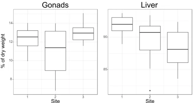
The total fat content of gonads is the highest at sampling site 3 (Figure 3.1), even though the difference is not significant. The lowest mean fat content in gonads was found at site 2. The highest fat content in livers was found at sampling site 1 and is decreasing then gradually towards sampling site 3. The difference between total fat content of livers at site 1 and 3 is significant (Kruskal-Wallis chi-squared = 8.4688, df = 30, p-value = 0.01449).

Figure 3.1:Total lipid contents of gonads (left) and livers (right). On the x axis are the three sampling sites. The y axis shows the fat content in percent of dry weight

3.1.2 Fatty acid profiles of gonads

Overall site 1 showed highest total amounts for gonad fatty acids in all 4 groups of fatty acids and highest values for Arachidonic acid and Docosahexaenoic acid (Figure 3.2). Significant are

the differences in the EPA:ARA ratio. Where site 3 has significantly higher values compared to both other sites (Kruskal-Wallis chi-squared= 12.808, df= 30, p-value= 0.001655, Pairwise Wilcoxon 3_1 p-value= 0.0078; 3_2 p-value= 0.0022). Between the amount of MUFAs of site 1 and both other sites, where site 1 has significantly larger amounts (Kruskal-Wallis chi-squared=

8.3226, df= 30, p-value= 0.01559, Wilcoxon 1_2 p-value= 0.028; 1_3 p-value= 0.027). The difference between total amount of gonad fatty acids (TFA) is significant in a Kruskal Wallis test (Kruskal-Wallis chi-squared= 6.5135, df= 30, p-value= 0.03851), but the post hoc Wilcoxon test is insignificant for the combination of all sites. Nevertheless, also other groups of fatty acids show trends of differences between the sites. The amount of ARA, is similar between site 1 and 2 with a mean of 12.83_mg^ng dry weight and 12.4_mg^ng and relatively lower at site 3 with a mean of 10.72_mg^ng dry weight. Looking at EPA on the other hand site 3 has the highest mean value (106.62_mg^ng dry weight) resulting in the highest EPA:ARA ratio of all sites (9.97). And site 2 has the lowest mean value for EPA (87.29_mg^ng). For DHA site 1 has the highest mean value with 123.1_mg^ng dry weight and site 2 and 3 have similar means of 100.46 and 108.17_mg^ng dry weight.

The saturated fatty acids are more or less the same at all sites, site 1 is slightly higher than the other two. This is the same for the PUFAs.

Figure 3.2:Box and whisker plot of the mount of the most important gonad fatty acids and fatty acid groups in ng/mg dry weight. The three sampling sites are displayed on the x axis. The y axis shows fatty acid amounts in ng/mg dry weight. Arachidonic acid (ARA), Eicosapentaenoic acid (EPA), Docosahexaenoic acid (DHA), saturated fatty acids (SFA), mono unsaturated fatty acids (MUFA), poly unsaturated fatty acids (PUFA), total fatty acids (TFA)

Results 23

The dominance of site 1, having the highest total values of gonad fatty acids in all four groups (SFAs, MUFAs, PUFAs, TFAs), is not pronounced in the percentage values for gonad fatty acids in proportion of the total fatty acid amount (TFA) (Figure 3.3). Only differences between Eicosapentaenoic acid and MUFAs are significant (Kruskal-Wallis EPA: chi-squared = 13.475, df = 30, p-value = 0.001186; Kruskal-Wallis MUFA chi-squared = 12.055, df = 30, p-value = 0.002411). Eicosapentaenoic acid values are highest at site 3 (Pairwise Wilcoxon EPA: 3_1 p=

0.00042, 3_2 p= 0.01026), as well as the differences between EPA:ARA ratios of site 3 and both other sites, as these stay the same as for the total values. Despite of having outliers the difference between site 1, which has the highest percentage contribution of MUFAs to total fatty acids, and both other sampling sites are significant (Pairwise Wilcoxon MUFA: 1_2 p=

0.0449, 1_3 p= 0.0025). In total contrast to the total values discussed before, PUFAs have the highest contribution to total fatty acids at site 3. And also, the values for Arachidonic acid shifted compared to the total values.

Figure 3.3: Box and whisker plot of the percentage contribution of the most important gonad fatty acids and fatty acid groups to total fatty acids (TFA). The three sampling sites are displayed on the x axis. The y axis shows fatty acid contribution in percent of total fatty acids. Arachidonic acid (ARA), Eicosapentaenoic acid (EPA), Docosahexaenoic acid (DHA), saturated fatty acids (SFA), mono unsaturated fatty acids (MUFA), poly unsaturated fatty acids (PUFA)

3.2 Condition indices and liver health

3.2.1 Condition indices

Table 3.1:Condition indices and fish parameters. Mean Hepatosomatic index (HSI), Gonadosomatic index (GSI), condition factor K, length in centimeters, age in years and weight in grams per site are listed with standard deviation. (Site 1 n= 12; Site 2 n= 10; Site 3 n= 10)

Site 1 Site 2 Site 3

n = 12 n = 10 n = 10

Age 6.167 ± 0.898 6.111 ± 1.197 7.273 ± 0.962

Weight 5990.583 ± 838.386 4782.500 ± 829.480 5709.545 ± 602.002

Length 84.750 ± 3.982 81.600 ± 3.878 84.000 ± 3.286

K 0.979 ± 0.059 0.873 ± 0.081 0.959 ± 0.067

HSI 10.462 ± 1.973 5.813 ± 2.269 5.362 ± 1.275

GSI 2.355 ± 0.333 1.361 ± 0.366 2.304 ± 0.979

Fish caught at site 2 were on average 3 cm shorter than at sites 1 and 3 (Table 3.1). Individuals at site 3 are about the same size, but one year older than individuals from site 1 and 2, which indicates a faster growth of individuals at site 1. The condition factor K is about 10 percent lower at site 2 compared to both other sites, but the difference was not significant in a Kruskal Wallis test. Site 1 and 3 show similar mean GSI values, the differences between GSI of site 2 and both other sites is significant (Kruskal-Wallis chi-squared = 17.899, df = 30, p-value = 0.0001298, Pairwise Wilcoxon 1_2 p-value= < 0.001, 2_3 p-value= 0.00049). Whereas the values for HSI are lower than at site 1 and even lower than at site 2 (Kruskal-Wallis chi-squared = 19.008, df

= 30, p-value = < 0.001, Pairwise Wilcoxon 1_2 p-value= 0.00031, 1_3 p-value= < 0.001, 2_3 p-value= 0.73936).

3.2.2 Liver parasites and tissue

Site 3 showed by far the highest amounts of macro liver parasites in proportion to the liver weight (mean parasite index of 0.62) and highest degrees of liver degeneration (Table 3.2). The parasite index between sites differs significantly (Kruskal-Wallis chi-squared = 14.152, df = 30, p-value

= 0.000845). The difference of the tissue indices between sites was insignificant in a Kruskal Wallis test, but showed significant differences between site 3 and both other sites in a post hoc Wilcoxon pairwise test (3_1 p-value= 0.0003; 3_2 p-value= 0.005).

Results 25

Table 3.2: Mean parasite indices and liver tissue indices per site are listed with standard deviation (Site 1 n= 12; Site 2 n= 10; Site 3 n= 10)

Site 1 Site 2 Site 3

Parasite Index 0.040 ± 0.020 0.082 ± 0.085 0.619 ± 0.494 Tissue Index 0.083 ± 0.276 0.600 ± 1.020 2.300 ± 0.640

Picture 3.4: 6 Liver macro parasites from an individual of site 1 (left) and an individual of site 3 (right)

3.3 Feeding patterns and stable isotopes

Prey indices between sites differed significantly (Figure 3.5, Table 3.3) (Kruskal-Wallis chi- squared = 22.766, df = 30, p-value = < 0.001). The prey composition of site 1 was mainly dominated by mesopelagic fish, a mix of crustaceans of which the habitat origin could not be determined properly andThemisto libellulaa pelagic amphipod (Figure 3.6). This is supported by prey indices of site 1 (average prey index= 2.5) (Table 3.3), which intend a prey composition of an unknown origin with a tendency to pelagic origin, driven by consumption of mesopelagic fish andThemisto libellua. Mesopelagic fish were only preyed at Site 1, with exception of two fish at site 3 (Fish ID 25, 26). Same forThemisto libelluawith the exception of two fish at site 2 (Fish ID 15, 17). Site 2 has a prey composition and an average prey index of 2.87, that suggests a pelagic food spectrum, being dominated by capelin (Mallotus villosus) and Euphausids. In contrast site 3 shows a clearly benthic dominated prey composition with an average prey index of 1.28 (Table 3.3). Main diet items at site 3 were benthic crabs (Hyas sp.), sea cucumbers (Holothuria) and brittle stars (Ophiuroidea). Four individuals of site 3 also had a proportion of pelagic food (Euphausiids, Hyperiidae and mesopelagic fish) in their stomachs (Fish 23, 24, 25, 26) (Figure Stomach content).

Figure 3.5: Prey indices for every individual fish and site. Colours indicate the main prey origin

Results 27

Figure 3.6:Species contribution (%) to the total stomach content weight of each individual. Uniden- tifiable, highly digested matter is combined as other remains. The Taxon Molluscs contains mainly Bivalvs, Gastropods and in some cases Theutids. Hard matter like stones and sand were combined as benthic remains. Colours and prey species are sorted by prey origin, pelagic on top, benthic on the bottom

A SIMPER analysis revealed capelin, crustaceans, euphausiids, mesopelagic fish,Hyassp.

and sea cucumbers as the most influential species (Supplementary). Site 1 shows the highest diversity in the prey composition with an average Shannon index of 1.19 for the stomach content analysis compared to 0.74 at site 3 and 0.72 at site 2 (Table Shannon and Prey index). Stomach content diversities are significantly different from each other (Kruskal-Wallis chi-squared = 8.2384, df = 30, p-value = 0.01626).

Table 3.3:Mean Shannon index of stomach contents per site and mean prey indices per site are listed with standard deviation. (Site 1 n= 12; Site 2 n= 10; Site 3 n= 10)

Site 1 Site 2 Site 3

Shannon Index 1.185 ± 0.415 0.718 ± 0.367 0.738 ± 0.439 Prey Index 2.523 ± 0.360 2.871 ± 0.153 1.277 ± 0.362

The stable isotope data show a clear seperation of site 3 from sites 1 and 2, with lower negative values forδC. Site 1 and 2 had similar values forδC andδN and are overlapping (Figure 3.7).

This is in consistency with the prey composition data from the stomach analyses, where site 1 and 2 are both driven by a pelagic food spectrum and site 3 by benthic feeding (Agurto 2007).

Three individuals from site 3 (Fish 24, 25, 26) are within the pelagic cluster of sites 1 and 2.

Interestingly, these three individuals were among the four fish with pelagic diet at site 3. One individual however from site 2 (Fish 22) is found in the benthic cluster of site 3 (Figure 3.7), but has no sign of benthic prey in the stomach content (Figure 3.6).

Figure 3.7: Stable isotope ratios of 30 fish, data for fish 4 and 7 were not available. On the x axis δC13 and on the y axisδN15. Sites are indicated by colour. a. is showing mean ratios of the sites, the error bars are showing the standard deviation. b. is showing the stable isotope signature for each individual. Numbers resemble FishID

3.4 Oceanography

Temperatures and salinity were obtained from corresponding stations with a maximum distance of ca. 31 km (Supplementary). Depth measurements were obtained from the net probe attached to the fishing gear. Sampling site 1 is the deepest station of all (Table 3.4). Site 3 is about 200 meters shallower than site 1 and the shallowest station of all. Because the data for site 1 was obtained from two different corresponding stations it shows a high variability in bottom (BT) and sea surface temperature (SST) within the site and minor variability in sea surface salinity (SSS). All other sites hat only one corresponding station. Low sea surface temperatures cooccur with lower sea surface salinities. The bottom salinities are around 35 PSU for all stations and are independent from bottom temperatures.

Results 29

All measured parameters were significantly different between the sites (Kruskal-Wallis, Depth:

chi-squared = 28.595, df = 2, p-value = < 0.001; BT: chi-squared = 22.589, df = 6, p-value = <

0.001; SST: chi-squared = 8.7891, df = 6, p-value = 0.01234; BS: chi-squared = 29.817, df = 6, p-value = < 0.001; SSS: chi-squared = 22.589, df = 6, p-value = < 0.001)

Table 3.4: Sampling sites and station properties. All sites with their sampling stations and number of sampled individuals are shown. Mean depth, sea surface temperature (SST) in degrees Celsius, bottom temperature (BT) in degrees Celsius, sea surface salinity (SSS) in practical salinity units (PSU) and bottom salinity (BS) in PSU are listed

Site 1 Site 2 Site 3

Station 691 692 693 694 719 720 721 751

Depth [m] 325 351.5 373.5 383 188.5 159 156.5 92

BT [^◦C] 1.037 1.037 4.757 4.757 4.429 4.429 4.429 5.574

SST [^◦C] 0.622 0.622 7.858 7.858 5.207 5.207 5.207 1.677

BS [PSU] 34.842 34.842 34.969 34.969 34.762 34.762 34.762 34.553 SSS [PSU] 32.443 32.443 34.773 34.773 34.311 34.311 34.311 31.952

Individuals Sampled 12♂ 10♂ 10♂

3.5 Regional influences on fatty acids

All variables included in this plot, were determined as the most influential species by using a SIMPER analysis. The first two dimensions explain 87.7% of the variance (Figure 3.8). All three sites differed in their biotic and abiotic patterns and are separated in their own clusters (Figure 3.9). The difference between site 1 and both other sites is driven by depth and MUFAs, being the deepest sampling station and having the highest total amounts (_mg^ng dry weight) and percentage contributions of MUFAs. The depth of the sampling station and the amount of PUFAs are not correlated. Total fatty acids, saturated fatty acids and C16:0 are subsets of each other and positively correlated. Individuals from site 2 and 3 have less amounts of all of the latter, whereas most individuals from site 1 are enriched.

Figure 3.8: Scree stack plot of the principal component analysis (PCA). The x axis shows the dimensions and the y axis shows the percentage of explained variance

Results 31

Figure 3.9: Principal component analysis of all parameters with data from 30 individual fish. Fish 4 and 7 are missing, due to a lack of stable isotope data. On the x axis dimension 1 and the percentage contribution of the dimension to the explained variance. On the y axis dimension 2 and the percentage contribution of the dimension to the explained variance. The single data points resemble the individual fish, colours indicate the sampling site. The vectors show the explanatory variables and their correlation between each other and the dimensions

The ANOVA function shows a significance for crustaceans (p-value= 0.042)(Supplementary), but overall no significance for any of the RDA axis. Sea cucumbers (Holothuria) andHyassp.

are positively correlated and share a quadrant (Figure 3.10). They show no correlation with euphausiids and capelin and a low negative correlation with crustaceans and mesopelagic fish and a high negative correlation with depth. Euphausiids and capelin share a quadrant and have a low negative correlation with depth and a high negative correlation with mesopelagic fish and crustaceans. Mesopelagic fish and crustaceans share a quadrant, both are also positively correlated with depth which has a quadrant of its own. Mesopelagic fish and crustaceans are associated with enrichments in Docosahexaenoic acid, Eicospentaenoic acid, C18:1n7, C16:1, C20:1n9c and C14:0. Capelin and euphausiids are depleted in these fatty acids. Depth is associated with an enrichment in C16:0, C18:0, and C18:1n9c. Sea cucumbers andHyassp. are associated with a depletion of these fatty acids.

Figure 3.10: Redundancy analysis (RDA) for explanatory variables that were chosen by a prior SIMPER analysis and all fatty acids

The ANOVA function shows a significance for crustaceans (p-value= 0.03), but overall no significance for any of the RDA axis (Supplementary). Euphausiids and capelin share a quadrant and are negatively correlated with mesopelagic fish and show almost no correlation with depth, crustaceans, sea cucumbers andHyassp. (Figure 3.11). Depth and crustaceans share a quadrant and are positively correlated with mesopelagic fish and negatively correlated withHyassp. and sea cucumbers. Hyassp. and sea cucumbers share a quadrant. They show no correlation with mesopelagic fish, which has a quandrant on its own. Depth and crustaceans are associated with saturated fatty acids (SFAs) and monounsaturated fatty acids (MUFAs) in their quadrant and are enriched in these groups of fatty acids. Mesopelagic fish joins total fatty acids (TFAs) and poly unsaturated fatty acids (PUFAs) in its quadrant and is associated with an enrichment in both of these fatty acid groups. Hyassp. and sea cucumbers are associated with high Eicosapentaenoic acid (EPA) to Arachidonic acid (ARA) ratios and are linked to a depletion in SFAs and MUFAs.

Euphausiids and capelin are linked with a depletion in PUFAs and TFAs.

Figure 3.11: Redundancy analysis (RDA) for explanatory variables that were shosen by a prior SIMPER analysis and all fatty acid groups plus the Eicosapentaenoic acid (EPA) to Arachidonic acid (ARA) ratio

4

Discussion

4.1 Lipids and fatty acids

Fatty acids are, due to their different chemical constitution, to a variate extent sensitive towards high temperatures, light and oxygen. Exposure to one or more of these factors enhance degra- dation and change fatty acid compositions (Myashita 2018), which should be considered in discussion. In order to prevent any potential sampling bias, fish tissue was processed as fast as possible and kept on ice during the whole procedure. Afterwards samples were stored contin- uously at at least -80^◦C, to minimize potential sources of errors. Total lipid contents of livers and therefore energy storage of cod, are highest at site 1 and decrease consecutively at the other two sites. These results are consistend with a previous study (Werner et al. 2018), where high condition of cod was linked to mesopelagic feeding in the area at and around site 1 (Dhorn Bank) (Figure 2.1). Total Lipid contents of gonads show a different pattern. In contrast to liver lipid contents, highest lipid contents in gonads were found at site 3. Even though the differences of gonad lipid content between sites are not significant, the combination of low liver lipid content and high gonad lipid content at site 3 indicates, that females at site 3 have a different maturity stage than females from the other sampling sites and low energy storages and bad condition were already linked to a shift in spawning times of Baltic sea cod (Tomkiewicz et al. 2010) and might also be possible for cod in Greenland waters. Consitent with high total lipid contents of livers, the total fatty acid (TFA) amounts (in Nanogram) in gonads are highest in individuals from sampling site 1. This also accounts for total amounts of all sub groups of fatty acids (SFAs, MUFAs and PUFAs), which showed highest values at site 1. Digging deeper in the important fatty acid group of PUFAs, the patterns become more complex. Total amounts of Arachidonic acid are lowest at site 3 and highest at site 1. Total amounts of Docosahexaenoic acid are highest at site 1. Amounts of Eicosapentaenoic acid are more balanced between the sites, but were highest at site 3. Low ARA values and high EPA values at site 3, result in the highest EPA:ARA ratio at site 3. Both of these patterns can also be seen in the percentage contributions of fatty acids to the total fatty acid amounts of gonads. Røjbek and colleagues (2012) who looked at lipid dynamics and reproductive cycles of Baltic Sea cod, found similar patterns in females, that were close to spawning. In their studies EPA levels stayed more or less constant over the year, but ARA levels were strongly decreasing towards spawning. This resulted in increased