Journal of
Marine Science and Engineering
Article
Spatial and Temporal Variability of Ice Algal Trophic Markers—With Recommendations about
Their Application
Eva Leu1,* , Thomas A. Brown2, Martin Graeve3 , Jozef Wiktor4 , Clara J. M. Hoppe3 , Melissa Chierici5,6, Agneta Fransson6,7, Sander Verbiest8,9, Ane C. Kvernvik8 and
Michael J. Greenacre1,10
1 Akvaplan-Niva, CIENS, Gaustadalléen 21, 0349 Oslo, Norway; michael.greenacre@gmail.com
2 Scottish Association of Marine Sciences, Oban PA37 1QA, UK; t2001b@hotmail.com
3 Alfred-Wegener-Institute, Helmholtz-Centre for Polar and Marine Research, 27570 Bremerhaven, Germany;
martin.graeve@awi.de (M.G.); clara.hoppe@awi.de (C.J.M.H.)
4 Institute of Oceanology Polish Academy of Science, 81-712 Sopot, Poland; wiktor@iopan.gda.pl
5 Institute of Marine Research, Fram Centre, 9007 Tromsø, Norway; melissa.chierici@hi.no
6 Department of Arctic Geophysics, University Centre of Svalbard, 9171 Longyearbyen, Svalbard, Norway;
agneta.fransson@npolar.no
7 Norwegian Polar Institute, 9296 Tromsø, Norway
8 Department of Arctic Biology, University Centre of Svalbard, 9171 Longyearbyen, Svalbard, Norway;
sanderverbiest@gmail.com (S.V.); AneK@unis.no (A.C.K.)
9 Department of Earth Sciences, Utrecht University, Heidelberglaan 8, 3584 Utrecht, The Netherlands
10 Department of Economics and Business, Universitat Pompeu Fabra, 08002 Barcelona, Spain
* Correspondence: eva.leu@akvaplan.niva.no
Received: 10 July 2020; Accepted: 21 August 2020; Published: 2 September 2020 Abstract:Assessing the relative importance of sea ice algal-based production is often vital for studies about climate change impacts on Arctic marine ecosystems. Several types of lipid biomarkers and stable isotope ratios are widely used for tracing sea ic-associated (sympagic) vs. pelagic particulate organic matter (POM) in marine food webs. However, there has been limited understanding about the plasticity of these compounds in space and time, which constrains the robustness of some of those approaches. Furthermore, some of the markers are compromised by not being unambiguously specific for sea ice algae, whereas others might only be produced by a small sub-group of species.
We analyzed fatty acids, highly branched isoprenoids (HBIs), stable isotope ratios of particulate organic carbon (POC) (δ13C), as well asδ13C of selected fatty acid markers during an Arctic sea ice algal bloom, focusing on spatial and temporal variability. We found remarkable differences between these approaches and show that inferences about bloom characteristics might even be contradictory between markers. The impact of environmental factors as causes of this considerable variability is highlighted and explained. We emphasize that awareness and, in some cases, caution is required when using lipid and stable isotope markers as tracers in food web studies and offer recommendations for the proper application of these valuable approaches.
Keywords: trophic marker; lipid; fatty acid; highly branched isoprenoid (HBI); IP25; H-Print; stable isotope ratio; compound-specific isotope analysis
1. Introduction
In a rapidly warming Arctic, primary production regimes are expected to change, and probably shift towards a larger contribution of phytoplankton, relative to sea ice algae, in response to increasingly
J. Mar. Sci. Eng.2020,8, 676; doi:10.3390/jmse8090676 www.mdpi.com/journal/jmse
J. Mar. Sci. Eng.2020,8, 676 2 of 24
open waters and thinning sea ice [1]. These changes are likely to have far-reaching implications for the entire marine ecosystem, although they often remain difficult to assess or predict in detail.
In the Bering Sea, a regime shift from a primarily benthic to a more pelagic food web has been observed over the past two decades and was attributed to decreased ice algal production [2,3]. The relevance of sea ice algal production for different parts of the polar ecosystem, ranging from key pelagic grazers to mammals has been studied extensively [4–7]. Another important aspect addressed in various studies has been assessing the overall strength of sympagic-pelagic or sympagic-benthic coupling [8–10].
Despite using different approaches, the key interest in all these studies is quantifying the relative importance of biomass produced by sea ice algae (as opposed to phytoplankton) for higher trophic level production. Different types of trophic markers are widely applied to analyze food web structure, based on numerous assumptions of how sea ice algae differ biochemically from phytoplankton. Here we will focus on two common types of trophic markers: (a) lipid-based trophic markers (fatty acid trophic markers, and highly branched isoprenoids), and (b)δ13C as one example of a stable isotope-based marker technique.
1.1. Fatty Acid Trophic Markers (FATM)
The repertoire of fatty acids in an algal cell is determined genetically and differs between major algal groups (for a recent review, see [11]). These fatty acids are taken up as part of a consumer’s diet, and partly incorporated unchanged into the lipids of animals at higher trophic levels. Hence, fatty acids can be used to trace the type of algae that an organism has been feeding on [12]. This concept works best for essential polyunsaturated fatty acids (PUFAs) that are synthesized de novo exclusively by algae in the marine food web, since other fatty acids found in higher organisms might be of non-algal origin. Furthermore, it has been shown that the relative abundances of fatty acids in algae may vary considerably depending on the environmental conditions, such as light, nutrient concentrations, and temperature [13–18]. Applying FATM to distinguish specifically between sea ice algae and phytoplankton as the source of lipids, however, is hampered by the fact that this distinction relies on the taxonomic composition of these two blooms being sufficiently distinct to be reflected in clearly different fatty acid profiles. However, quite frequently diatoms account for the dominating part of the biomass in both pelagic and sympagic spring blooms.
1.2. Highly Branched Isoprenoids (HBIs)
Produced only by diatoms, HBIs are alkene biomarkers that have been used increasingly as specific indicators for sea ice algae, both in food web studies, but also as paleo-proxies for studying the position of the sea ice edge in the past [19,20]. Some HBIs are produced specifically by a number of Arctic pennate diatoms including species within the genera ofHaslea, Pleurosigma,andRhizosolenia[19,21].
A monounsaturated HBI with 25 carbon atoms was identified as specific to a subset of Arctic sea ice diatoms [19,22] and termed the ”Ice Proxy” or IP25 [20] IP25 is chemically stable and becomes incorporated unaltered into organisms at higher trophic levels and, due to its source specificity, is an excellent tracer for carbon fixated by sea ice algal primary production. The distribution of IP25in sea ice broadly corresponds to the ice algal bloom peak, with the highest concentrations being measured nearer the ice-water interface and mostly in the lower 1–5 cm horizon of sea ice [23,24]. The diatom species producing this compound usually account for 1–5% of sea ice diatoms, while the most dominant species (e.g.,Nitzschiaspp.) are not producing it [19]. Alongside IP25, a suite of HBI isomers have been identified as providing specific indicators for either pelagic or sympagic microalgae [25]. This enabled the development of an index for the relative proportion of sympagic to pelagic HBIs, the so-called H-Print [26]. Recently, the production rate of certain HBIs was found to increase strongly under nutrient limiting conditions in the sea ice diatomHaslea vitrea, indicating some sort of environmental control of the cellular content of these compounds [27].
J. Mar. Sci. Eng.2020,8, 676 3 of 24
1.3. Carbon Stable Isotope Ratios (δ13C)
A further trophic marker approach used to identify sea ice algae is based on the ratio between the two stable isotopes of carbon,12C and13C, expressed asδ13C (%). This ratio is widely applied in trophic food web analyses, but the basis for its specific use to contrast sea ice algae vs. phytoplankton is the relative shortage of inorganic carbon for photosynthesis in spatially limited brine channels where high biomass densities might accumulate, as opposed to a usually well replenished surface layer of the ocean. As a result,δ13C values in sympagic algae become enriched over time by13C. A strong impact of both nutrient availability as well as taxonomic composition on sympagic particulate organic carbon (POC)δ13C was described previously [28], and the implications for tracing the fate of ice algal production in Arctic food webs is discussed extensively both in this work, as well as more recently [29].
One caveat of this approach is that Arctic phytoplankton can also exhibit considerable base-line variation in its isotope values which can result in overlaps with sea ice algae, complicating food- web analyses [30].
In order to mitigate some of the shortcomings of the above described approaches, and to increase the specificity, it is possible to measureδ13C values not only for total POC, but also for specific compounds, such as individual fatty acids (termed compound-specific isotope analysis, CSIA of fatty acids, FAs). This approach has been successfully applied to Arctic and Antarctic food webs [7].
For example, a combination of FATM and CSIA of FAs was used to describe and distinguish between ice-associated and pelagic particulate organic matter (i-POM vs. p-POM) in a study from the Bering Sea [31].
Allof these analytical methods and approaches have their specific advantages and shortcomings, which will be discussed in the later part of this article. Although large-scale food-web analyses understandably require some level of generalization, it is crucial to be aware that none of these markers in primary producers are constant. Rather, their occurrence and abundance depend strongly on both taxonomic composition and physiological status of the organism in question, which ultimately are controlled by environmental conditions and concurrent growth phase. For isotopic signatures in bottom sea ice POC and particulate organic nitrogen (PON), such interactions were described and discussed thoroughly previously [28].
There is some information available on the dynamics of some of these markers on both species, and even more importantly, community level; however, studies measuring all of them simultaneously are very rare. Spring bloom dynamics of primary producers in high latitudinal ecosystems are highly unpredictable and quite dynamic, and we therefore expect correspondingly high variability in the trophic marker signatures during pre-, peak- and post-bloom stages. The aim of our study was to document the spatial and temporal variability of different lipid and stable isotope-based trophic markers during an ice algal spring bloom and relate it to environmental conditions, as well as taxonomic composition. We then used these data to compare and contrast the reliability of each approach to distinguish between sympagic and pelagic POM.
2. Materials and Methods
All data were collected during spring/summer 2017 as part of the FAABulous project (Future Arctic Algae Blooms—and their role in the context of climate change) in Van Mijenfjorden in Svalbard (Norway).
2.1. Site Description
Located on the western coast of Spitsbergen, Van Mijenfjorden has maximum water depths ranging from ca. 70 m in the inner basin to ca. 100 m in the outer basin and is semi-closed by the Akseløya island (Figure1), located close to its entrance. Together with a shallow sill, this island limits the inflow of Atlantic water such that stable ice cover can form within the fjord from December/January until June/early July [32]. Due to the strongly increased winter temperatures in Svalbard, however, ice formation has become more variable and weaker during the past 10–15 years, resulting in a shorter period of ice
J. Mar. Sci. Eng.2020,8, 676 4 of 24
coverage [33]. In 2017, sea ice started to form and stabilize around the end of January/early February in the innermost part of the fjord, but did not reach thicknesses (>0.2–0.3 m) that allowed safe working conditions before early March. A sea ice observatory was installed close to the deepest part of the inner basin on 8th of March providing background data for the entire study period on sea ice thickness, snow cover, and transmittance. Sea ice algal development was followed by sampling different stations in the inner basin from early March to early May 2017, including a spatial transect starting from a very shallow station close to the shore (IS) to the mid-fjord station VMF2 (Figure1).
J. Mar. Sci. Eng. 2020, 8, x FOR PEER REVIEW 4 of 25
the end of January/early February in the innermost part of the fjord, but did not reach thicknesses (>0.2–0.3 m) that allowed safe working conditions before early March. A sea ice observatory was installed close to the deepest part of the inner basin on 8th of March providing background data for the entire study period on sea ice thickness, snow cover, and transmittance. Sea ice algal development was followed by sampling different stations in the inner basin from early March to early May 2017, including a spatial transect starting from a very shallow station close to the shore (IS) to the mid-fjord station VMF2 (Figure 2).
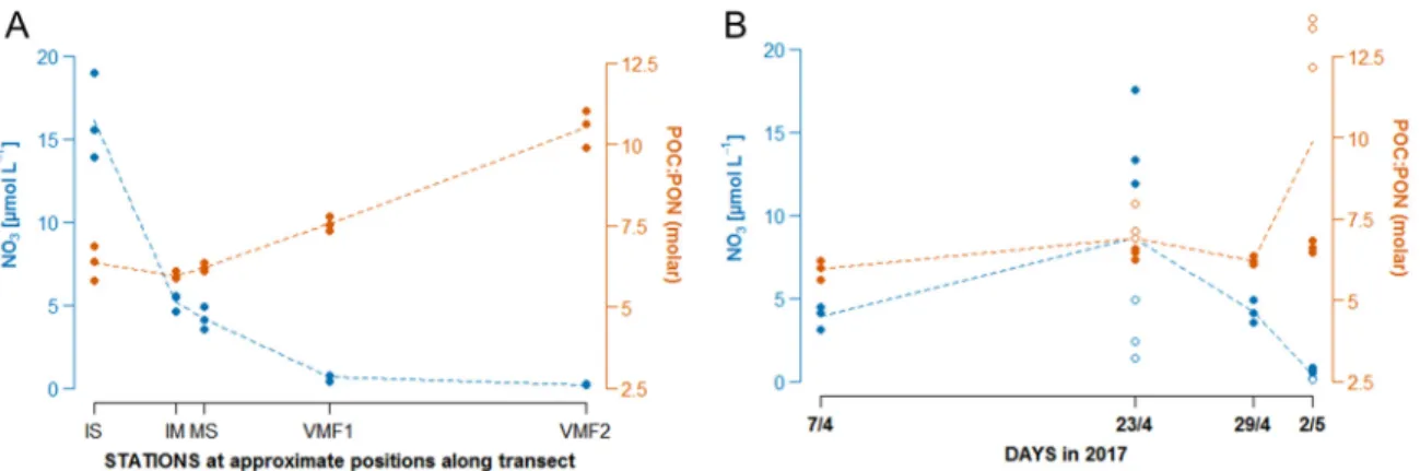
Figure 1. Nitrate concentrations (µmol L−1) and molar ratios of POC to particulate organic nitrogen (PON) along the transect (A) and changing over time (B). In the time series data, localities with low and high snow were sampled specifically on two occasions (23/4 and 2/5), clearly displaying distinct C:N ratios and nutrient concentrations (open symbols: low snow, filled symbols: high snow).
Trendlines were inserted based on overall average values of all samples taken on a given day (n = 3–
6).
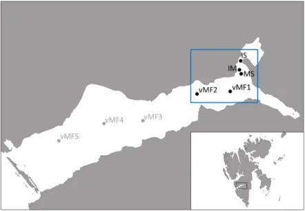
Figure 2. Sampling transect of the FAABulous project in Van Mijenfjorden, Svalbard. The sea ice samples were taken from the five innermost stations (IS, IM, MS, VMF1, VMF2) as sea ice coverage was rather poor and not covering the entire fjord in winter/spring 2016/2017.
2.2. Sampling
Sampling was conducted on landfast ice near the settlement of Svea, in Van Mijenfjorden, Spitsbergen from 3 March to 2 May 2017. Sea ice core samples (bottom 0–3 cm) were usually collected from an area covered by intermediate snow (8–15 cm) using a 9 cm internal diameter core barrel (Kovacs Mark II). In some occasions where snow cover appeared very variable, separate sets of
Figure 1. Sampling transect of the FAABulous project in Van Mijenfjorden, Svalbard. The sea ice samples were taken from the five innermost stations (IS, IM, MS, VMF1, VMF2) as sea ice coverage was rather poor and not covering the entire fjord in winter/spring 2016/2017.
2.2. Sampling
Sampling was conducted on landfast ice near the settlement of Svea, in Van Mijenfjorden, Spitsbergen from 3 March to 2 May 2017. Sea ice core samples (bottom 0–3 cm) were usually collected from an area covered by intermediate snow (8–15 cm) using a 9 cm internal diameter core barrel (Kovacs Mark II). In some occasions where snow cover appeared very variable, separate sets of samples were taken from areas with high (<15 cm) and low (<5 cm) of snow. Natural heterogeneity in sea ice core protists biomass [34] was overcome by collecting 3 replicate samples, each consisting of 1–6 pooled ice core bottom slices for each sampling day. All sea ice cores were melted with addition of 0.7µm filtered seawater (9 parts FSW to 1 part melted ice) to minimize osmotic stress on the microbial community during melting [35]. Once melted, ice core samples were filtered (GF/F), filters were wrapped in aluminum foil and stored in liquid nitrogen. Two additional ice cores were obtained for each sampling date: one to measure the ice temperature and salinity to estimate brine volume, the other for analyzing inorganic nutrients (see below). For total dissolved inorganic carbon (DIC) in sea ice, ice cores were collected using the same ice corer (Kovacs, Ø=0.09 m), where the full length ice cores were directly placed in long-sleeve plastic bags and put into a−20◦C freezer for short-term storage (few days), and further transport to the laboratory at the University Centre in Svalbard (UNIS, Longyearbyen). In the laboratory, the ice cores were cut into 10 cm sections, where only the bottom 10 cm of the bulk sea-ice (hereafter referred to as sea ice) was used. The ice pieces were immediately transferred to gastight Tedlar bags to initiate the ice melting as soon as possible. The sea-ice samples were thawed in a cool and dark place with a melting time of approximately 24–48 h. Samples from the water column were taken with a Niskin bottle from discrete depths (5, 10, 15, 25, and 50 m), in addition, surface water from directly underneath the sea ice was sampled with a manual hand pump. The water samples were kept cold and dark, and filtered within a few hours after each field trip;
J. Mar. Sci. Eng.2020,8, 676 5 of 24
further sample analysis procedures were identical to sea ice samples. Due to low biomass in the deeper samples, samples from several depths had to be pooled for trophic marker analysis in order to obtain sufficient biomass.
2.3. Organic Carbon Analysis
Particulate organic carbon (POC) and nitrogen (PON) of sea ice algae were measured after filtration onto pre-combusted (4 h, 450◦C) GF/F filters (Whatman). Filters were stored at−20◦C and soaked with 200 mL 0.2 M HCl (Merck) to remove inorganic carbon. Filters were dried for at least 12 h at 60◦C prior to sample preparation. Analysis was performed using a CHNS-O elemental analyzer (Euro EA 3000, HEKAtech) which was calibrated using acetanilide standards. Contents of POC and PON were corrected for blank measurements and normalized to filtered volume and cell densities to yield cellular quotas.
2.4. Lipid Analysis
For lipid analysis, 9-octyl-8-heptadecene (10µL; 0.5µg mL−1) internal standard was added to filters in combination with nonadecanoic acid (10µL; 1 mg mL−1) for quantification of HBIs and fatty acids respectively from sea ice (36–145 mL filtered). Filters were then saponified (5% KOH;
70◦C; 60 min), after which non-saponifiable lipids (including HBIs) were extracted with hexane (3 ×2 mL) and purified by open column chromatography (SiO2; 3 column volumes of hexane).
Combined hexane extracts were dried using N2. Fatty acids were obtained by adding concentrated HCl (1 mL) to the saponified solution (after extraction of non-saponifiable lipids) and re-extracted with hexane (3×2 mL). Identification of HBIs was achieved following analysis by selective ion monitoring (SIM;m/z350.3,m/z348.3, andm/z346.3; limit of detection=1 ng L−1) using a Shimadzu QP2010 gas chromatograph coupled to a QP2020 quadrapole EI mass spectrometer (GC-MS; HP5ms; [36]).
Comparison of HBIs in sample extracts to the retention index and mass spectra obtained from standard extracts and literature provided unambiguous identification. Molecule structures and nomenclature of the analyzed HBI compounds are summarized in Figure S1. Fatty acids were derivatized to methyl esters by the addition of HCl:MeOH (1 mL; 1:9) and heating (70◦C; 60 min). Fatty acid methyl esters were re-extracted with hexane (3×2 mL) and analyzed at the Alfred Wegener Institute (AWI) using a gas chromatograph (GC-6890N, Agilent Technologies) equipped with an automatic sampler fitted with a J&W DB-FFAP column (60 m, 0.25 mm internal diameter, 0.25µm film). Inlet and FID detector temperatures were set at 250 and 260◦C, respectively. Helium was used as a carrier gas in constant flow mode at an average linear velocity of 25 cm sec−1. Oven temperature started at 80◦C for 2 min, then increased following two ramps (up to 160◦C at 20◦C min−1, and then up to 240◦C at 2◦C min−1) with a final hold time of 20 min at 240◦C. Individual fatty acids were identified by comparing relative retention times with those of a known standard mixture derived from Arctic and Antarctic copepods.
For quantification, HBI abundances were normalized according to a response factor (Belt et al. 2012), and both HBIs and fatty acids were further normalized to quantities of internal standards and sample mass or volume as required. Quantification was carried out on peaks with s/n=≥3.
2.5. Bulk Stable Isotope Analysis
All samples for isotope compositions were analyzed using an elemental analyzer (Flash 2000, Thermo Scientific, Milan, Italy) coupled to an isotope ratio mass spectrometer (Delta V Plus with a Conflo IV interface, Thermo Scientific, Bremen, Germany). Analyses were conducted at the Littoral, Environment and Societies Joint Research Unit stable isotope facility (University of La Rochelle, France).
Results are expressed in theδnotation as deviations from standards (Vienna Pee Dee Belemnite forδ13C and N2 in air forδ15N) following the formula:δ13C orδ15N=((Rsample/Rstandard)−1)×103, where R is
13C/12C or15N/14N. Prior to isotope analysis ofδ13C, carbonates were removed by adding a few drops of HCl 0.2 mol L−1until cessation of bubbling. Subsequently, samples were dried at 60◦C. Calibration was done using reference materials (USGS-24, -61, -62, IAEA-CH6, -600 for carbon; USGS-61, -62,
J. Mar. Sci. Eng.2020,8, 676 6 of 24
IAEA-N2, -NO-3, -600 for nitrogen). The analytical precision of the measurements was<0.15%for carbon and nitrogen based on analyses of USGS-61 and USGS-62 used as laboratory internal standards.
This method allows obtainingδ15N values in parallel, but we will report onδ13C values only.
2.6. Compound-Specific Isotope Analysis of Fatty Acids
Theδ13C isotopic composition in FAs was measured using a Thermo gas chromatography- combustion isotope-ratio mass spectrometry (GC-c-IRMS) system (Thermo Scientific) (see [37]).
For each analytical run, 2 reference gas pulses were used for data calibration at the start and at the end, together with the internal standard 23:0 FA methyl ester (FAME) (δ−32.50%, Pee Dee Belemnite (PDB)).
The chromatographic peak areas and carbon isotope ratios were obtained with the instrument-specific software (Isodat 3.0), and the certified reference standards 14:0 and 18:0 FAME (Iowa University) were used with knownδ13-values for further calculations.
2.7. Sea Ice Algae Taxonomy
Subsamples of 100–200 mL were fixed with a mixture of glutaraldehyde and Lugol’s solution (both 2% final concentration) for qualitative and quantitative analyses. Taxonomic identification of sea ice algal species was carried out on each ice core sample using the Utermöhl method [38]. As sea ice samples were so dense, 0.5 mL of sample were suspended in 9.95 mL of artificial seawater (to ensure uniform settling on the bottom of the chamber), and then a 10 mL Utermöhl chamber was used. Species identification and countings were carried out using an inverted microscope (Nikon TE-300 under magnifications of 100×and 600×), equipped with phase and interference contrasts and a picture acquisition system (NisElements BR). Taxa>20µm were counted on the entire chamber surface under 100×magnification. The cells were counted in an ocular photomask frame of a known area along the transect crossing the bottom chamber surface. Cells<20µm were counted under 400–600× magnification on 3 parallel transects. Biovolume calculations were done based on stereogeometric shapes measurements and calculated according to the HELCOM Phytoplankton Expert Group (PEG) biovolume spreadsheet. Conversions to biomass were done according to Menden & Deuer [39].
More detailed examination of certain taxa was achieved by dry-mounting sub-samples of cleaned (10% HCl; 70◦C for 30 min and 3×10 mL Milli-Q washes) cells and examination using a JEOL 7001F scanning electron microscope. In addition, diatoms belonging to theHasleagenus with known ability to produce IP25, specifically, were identified based upon general morphological dimensions in addition to features considered characteristic of the genus including, for example, the presence of external longitudinal strips over many areolae, with intervening continuous slits.
2.8. Determination of Inorganic Nutrient Concentrations
Ice core sections for nutrient analysis were thawed without addition of filtered seawater in the dark within appx. 24 h. Nutrient samples were filtered using acid washed syringes (10% HCl, 48 h) and GF/F filters. Samples were stored in 15 mL acid washed Falcon tubes at−20◦C until further analysis.
After thawing, the concentrations of nitrate, phosphate, and silicate were measured colorimetrically on a QuaAAtro autoanalyzer (Seal Analytical, Mequon, WI, USA) using internal calibrations and CRMs (KANSO, Osaka, Japan) for quality control.
2.9. Determination of Total Dissolved Inorganic Carbon
The thawed sea ice was transferred to 250 mL borosilicate glass bottles. Saturated mercuric chloride was added to the melted sea ice (60µL for 250 mL) to halt biological activity. Samples were analyzed for DIC at the Institute of Marine Research, Tromsø, Norway. Analytical methods for DIC determination in seawater samples are described in [40]. DIC was determined using gas extraction of acidified samples followed by coulometric titration and photometric detection using a Versatile Instrument for the Determination of Titration carbonate (VINDTA 3C, Marianda, Germany). Routine analyses of Certified Reference Materials (CRM, provided by A. G. Dickson, Scripps Institution of Oceanography,
J. Mar. Sci. Eng.2020,8, 676 7 of 24
USA) ensured the accuracy and precision of the measurements. The average standard deviation from triplicate CRM analyses was within±1µmol kg−1.
2.10. Determination of Chlorophyll a (Chl a)
Samples for Chl a determination were filtered onto GF/F filters (Whatman, Maidstone, UK) using a gentle vacuum, shock frozen in liquid nitrogen, and stored at−80◦C until further analysis.
For analysis filters were extracted in 10 mL methanol for 24 h at+4◦C in darkness and measured on a 10-AU-005-CE Fluorometer (Turner Designs, San Jose, CA, USA).
2.11. Statistical Analysis
All data analysis was conducted using R 3.5.0 (R Core Team 2018: R: a language and environment for statistical computing. R Foundation for Statistical Computing, Vienna, Austria. URL: https:
//www.R-project.org/). Compositional bar charts were used to show the changing species composition across the transect, and also, specifically for station MS, the changing composition over the period 4 April–2 May 2017. Similarly, scatter plots were used to show different variables along the transect, and again specifically for station MS, their values for the short time series. To compare the ice and pelagic samples for several variables at the same time, either canonical correspondence analysis (CCA, for compositional variables) or redundancy analysis (RDA, for interval-scale variables) was used, where the solution was constrained to show the ice-pelagic contrast on the first dimension. The package
”vegan” (Oksanen J, Blanchet FG, Friendly M, Kindt R, Legendre P, McGlinn D, Minchin PR, O’Hara R.B., Simpson GL, Solymos P, Stevens HH, Szoecs E, Wagner H. 2019. vegan: Community Ecology Package.
R package version 2.5–6,https://CRAN.R-project.org/package=vegan(last accessed 30 March 2020)) was used to conduct a multivariate permutation test on this dimension, thereby testing the ice-pelagic difference in a multivariate framework. To further investigate the correlation between different trophic markers and nutrient concentrations or stoichiometry, Spearman rank correlations were computed due to the nonlinear relationships observed in the scatterplots of the variables. Thep-values for the correlations are estimated using a distribution-free permutation test [41], as implemented in the function perm.cor.test in the R package jmuOutlier (Garren ST 2019. jmuOutlier: Permutation Test for Nonparametric Statistics. URLhttps://CRAN.R-project.org/package=jmuOutlier). Because of multiple testing, the Benjamini-Hochberg step-up procedure was used to avoid false positives at the overallp=0.05 level [42,43].
3. Results
3.1. General Physical Situation, Development of Chl a, Nutrients and C:N Ratios along the Transect and over Time Sea ice algae abundance and taxonomy were studied from early March to early May, but only from April onwards did biomass concentrations become high enough to measure all trophic markers in sea ice samples. Sea ice thickness varied from 30 to 50 cm, and snow cover on top of the ice was between 0 and 27 cm. For a more detailed description of the general situation, including algal physiology see [44].
In short, highest sea ice Chl a concentrations at the main study station (MS) were measured on April 23rd with up to 260µg L−1, whereas 160–170µg Chl a L−1were measured on 29th April and 2nd of May (Table1). With respect to POC concentrations, the highest concentrations were found on the 23rd of April and 2nd of May, with 8–10 mg L−1. Interestingly, the POC:Chl a ratio clearly reflected the impact of increased light under lower snow cover, and increased from 23 (23/4, high snow cover) to 93 (2/5, no snow) within only two weeks. Along the transect, Chl a concentrations varied between 120 and 190µg L−1, with only VMF2 being much lower (44µg L−1), while POC concentrations ranged from 2.5 (VMF2) to 13.7 mg L−1(IS). Concentrations of diatom lipids (Σof 16:1(n-7), C16 PUFAs, 20:5(n-3)) were highest at the shallow IS station (178 ng mL−1), and lowest at MS (25 ng mL−1).
Normalized to POC, however, the highest amounts were found at VMF2 (39 ng (µg POC) mL−1).
Nutrient concentrations in sea ice were declining over time – in particular for nitrate and silicate.
J. Mar. Sci. Eng.2020,8, 676 8 of 24
Along the transect, the highest silicate concentrations were measured in the areas with shallowest water depth, namely stations IS and IM, with 1.6 and 1.5µmol L−1, respectively. At other locations concentrations were<1µmol L−1. At station IS, the highest nitrate concentration in ice was detected (16µmol L−1), followed by IM (5.2µmol L−1) and MS (4.2µmol L−1, Table1). Dissolved inorganic carbon (DIC) concentrations were measured only at MS, VMF1, and VMF2. At the end of April, DIC was highest at the MS station (344 µmol kg−1) and decreased to its lowest values at VMF2 (319µmol kg−1). Time series measurements of environmental parameters conducted at sampling station MS showed rather similar patterns. Highest DIC concentrations of 387µmol kg−1 were observed at the beginning of April and then decreased, most rapidly between 23rd of April to 2nd of May, from 369 to 337µmol kg−1. The lower DIC coincided with decreasing nitrate concentrations.
Nitrate first only declined slowly from early April (approx. 4µmol L−1) to the 23rd of April (3µmol L−1).
Under high snow cover, even concentrations of 14µmol L−1 were measured on that day, maybe indicating a slower sea ice algal bloom development under high snow cover. However, on the 2nd of May, nitrate was substantially reduced to concentrations below 1µmol L−1. Interestingly, a similarly strong gradient of nitrate concentrations was found along the transect, ranging from 15–16µmol L−1 at the shallowest station (IS) to<0.2µmol L−1at VMF2 (Table1). Silicate concentrations at most of the stations and sampling events were rather depleted, well below 1µmol L−1, with the only exception being the shallowest area of the transect (stations IS and IM), where values between 1.5 and 2µmol L−1 were found. Phosphate concentrations varied between 0.3 and 1.5µmol L−1without any clear spatial or temporal trend.
Molar ratios of POC to PON. Particulate carbon to nitrogen ratios displayed a distinct spatial pattern, with values around 6–7, close to Redfield proportions, at the three innermost stations (IS, IM, MS), and clearly higher values at VMF1 and VMF2 (i.e., almost twice as high, Figure2A).
This corresponds well with the different nitrate concentrations measured in sea ice (see Table 1, Figure2A), where stations VMF1 and VMF2 were almost completely depleted for nitrate. Again, this spatial pattern resembled the main trend in the temporal development at MS, with a development towards nitrated depletion and increased POC:PON ratios in early May, even more pronounced at the sampling location with little to no snow coverage (Figure2B).
J. Mar. Sci. Eng. 2020, 8, x FOR PEER REVIEW 4 of 25
the end of January/early February in the innermost part of the fjord, but did not reach thicknesses (>0.2–0.3 m) that allowed safe working conditions before early March. A sea ice observatory was installed close to the deepest part of the inner basin on 8th of March providing background data for the entire study period on sea ice thickness, snow cover, and transmittance. Sea ice algal development was followed by sampling different stations in the inner basin from early March to early May 2017, including a spatial transect starting from a very shallow station close to the shore (IS) to the mid-fjord station VMF2 (Figure 2).
Figure 1. Nitrate concentrations (µmol L−1) and molar ratios of POC to particulate organic nitrogen (PON) along the transect (A) and changing over time (B). In the time series data, localities with low and high snow were sampled specifically on two occasions (23/4 and 2/5), clearly displaying distinct C:N ratios and nutrient concentrations (open symbols: low snow, filled symbols: high snow).
Trendlines were inserted based on overall average values of all samples taken on a given day (n = 3–
6).
Figure 2. Sampling transect of the FAABulous project in Van Mijenfjorden, Svalbard. The sea ice samples were taken from the five innermost stations (IS, IM, MS, VMF1, VMF2) as sea ice coverage was rather poor and not covering the entire fjord in winter/spring 2016/2017.
2.2. Sampling
Sampling was conducted on landfast ice near the settlement of Svea, in Van Mijenfjorden, Spitsbergen from 3 March to 2 May 2017. Sea ice core samples (bottom 0–3 cm) were usually collected from an area covered by intermediate snow (8–15 cm) using a 9 cm internal diameter core barrel (Kovacs Mark II). In some occasions where snow cover appeared very variable, separate sets of
Figure 2.Nitrate concentrations (µmol L−1) and molar ratios of POC to particulate organic nitrogen (PON) along the transect (A) and changing over time (B). In the time series data, localities with low and high snow were sampled specifically on two occasions (23/4 and 2/5), clearly displaying distinct C:N ratios and nutrient concentrations (open symbols: low snow, filled symbols: high snow). Trendlines were inserted based on overall average values of all samples taken on a given day (n=3–6).
J. Mar. Sci. Eng.2020,8, 676 9 of 24
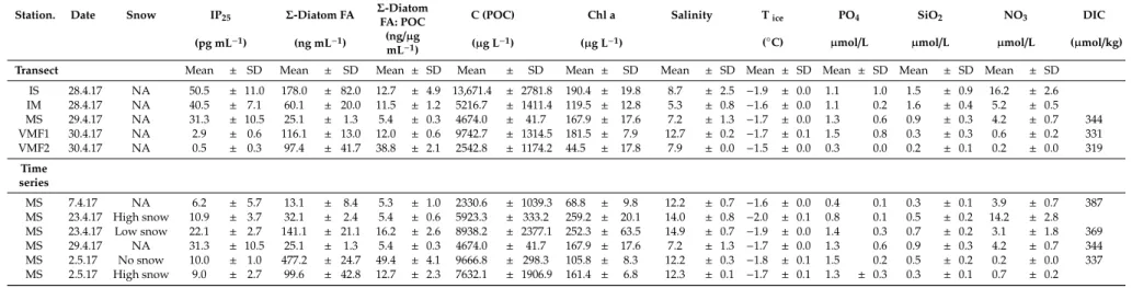
Table 1.Physico-chemical and biological characteristics of bottom sea ice (0–3 cm) sections with respect to nutrients, dissolved inorganic carbon, DIC, temperature, salinity, algal biomass (measured as particulate organic carbon, POC, and chlorophyll a, Chl a), as well as lipids along the transect, and for the time series. Shown are means and SD (n=3).
Station. Date Snow IP25 Σ-Diatom FA Σ-Diatom
FA: POC C (POC) Chl a Salinity Tice PO4 SiO2 NO3 DIC
(pg mL−1) (ng mL−1) (ng/µg
mL−1) (µg L−1) (µg L−1) (◦C) µmol/L µmol/L µmol/L (µmol/kg)
Transect Mean ± SD Mean ± SD Mean ± SD Mean ± SD Mean ± SD Mean ± SD Mean ± SD Mean ± SD Mean ± SD Mean ± SD
IS 28.4.17 NA 50.5 ± 11.0 178.0 ± 82.0 12.7 ± 4.9 13,671.4 ± 2781.8 190.4 ± 19.8 8.7 ± 2.5 −1.9 ± 0.0 1.1 1.0 1.5 ± 0.9 16.2 ± 2.6
IM 28.4.17 NA 40.5 ± 7.1 60.1 ± 20.0 11.5 ± 1.2 5216.7 ± 1411.4 119.5 ± 12.8 5.3 ± 0.8 −1.6 ± 0.0 1.1 0.2 1.6 ± 0.4 5.2 ± 0.5
MS 29.4.17 NA 31.3 ± 10.5 25.1 ± 1.3 5.4 ± 0.3 4674.0 ± 41.7 167.9 ± 17.6 7.2 ± 1.3 −1.7 ± 0.0 1.3 0.6 0.9 ± 0.3 4.2 ± 0.7 344
VMF1 30.4.17 NA 2.9 ± 0.6 116.1 ± 13.0 12.0 ± 0.6 9742.7 ± 1314.5 181.5 ± 7.9 12.7 ± 0.2 −1.7 ± 0.1 1.5 0.8 0.3 ± 0.3 0.6 ± 0.2 331
VMF2 30.4.17 NA 0.5 ± 0.3 97.4 ± 41.7 38.8 ± 2.1 2542.8 ± 1174.2 44.5 ± 17.8 7.9 ± 0.0 −1.5 ± 0.0 0.3 0.0 0.2 ± 0.1 0.2 ± 0.0 319
Time series
MS 7.4.17 NA 6.2 ± 5.7 13.1 ± 8.4 5.3 ± 1.0 2330.6 ± 1039.3 68.8 ± 9.8 12.2 ± 0.7 −1.6 ± 0.0 0.4 0.1 0.3 ± 0.1 3.9 ± 0.7 387
MS 23.4.17 High snow 10.9 ± 3.7 32.1 ± 2.4 5.4 ± 0.6 5923.3 ± 333.2 259.2 ± 20.1 14.0 ± 0.8 −2.0 ± 0.1 0.8 0.1 0.5 ± 0.2 14.2 ± 2.8 MS 23.4.17 Low snow 22.1 ± 2.7 141.1 ± 21.1 16.2 ± 2.6 8938.2 ± 2377.1 252.3 ± 63.5 14.9 ± 0.7 −1.9 ± 0.0 1.4 0.3 0.7 ± 0.2 3.1 ± 1.8 369
MS 29.4.17 NA 31.3 ± 10.5 25.1 ± 1.3 5.4 ± 0.3 4674.0 ± 41.7 167.9 ± 17.6 7.2 ± 1.3 −1.7 ± 0.0 1.3 0.6 0.9 ± 0.3 4.2 ± 0.7 344
MS 2.5.17 No snow 10.0 ± 1.0 477.2 ± 24.7 49.4 ± 4.1 9666.8 ± 298.3 105.8 ± 8.3 12.2 ± 0.3 −1.8 ± 0.1 1.5 0.2 0.5 ± 0.2 0.2 ± 0.0 337 MS 2.5.17 High snow 9.0 ± 2.7 99.6 ± 42.8 12.7 ± 2.3 7632.1 ± 1906.9 161.4 ± 6.8 12.3 ± 0.1 −1.7 ± 0.1 1.3 ± 0.3 0.3 ± 0.1 0.7 ± 0.2
J. Mar. Sci. Eng.2020,8, 676 10 of 24
3.2. Species Composition
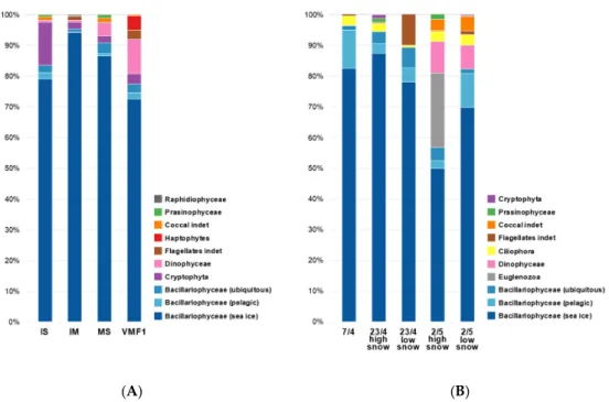
Results from the analysis of ice algal species composition along the transect (available for all stations apart from VMF2) revealed that diatoms (Bacillariophyceae) accounted for 76–89% of the total algal biomass at all stations (Figure 3). Diatoms almost exclusively comprised pennate species, with the vast majority being typical ice-associated species, without any clear spatial trend. There was some variability between replicates at sampling sites and sampling stations, with Chrysophyceae being the second most important group at the shallow coastal site (IS station) and accounting for 17%.
At the remaining three stations, dinoflagellates were the algal group that was second most dominant, accounting for 13–20% of total algal biomass. Prymnesiophyceae were only found at VMF1 (about 4% of total biomass). Other groups represented only very minor contributions to the overall algal biomass (Figure3A). Following the species composition data from early April to early May at the main station (MS), similar patterns are visible: Bacillariophyceae account for 70 to>95% of the total algal biomass, with one notable exception being the sample taken on the 2nd of May under low/no snow conditions (Figure3B). Here, the sympagic EuglenozoaAnisonemasp. accounted for almost 25% of the total biomass. Within the Bacillariophyceae, pennates were by far most abundant, and classified ice-associated species outnumbering pelagic ones (50–87% vs. 3–12%).
J. Mar. Sci. Eng. 2020, 8, x FOR PEER REVIEW 10 of 25
Molar ratios of POC to PON. Particulate carbon to nitrogen ratios displayed a distinct spatial pattern, with values around 6–7, close to Redfield proportions, at the three innermost stations (IS, IM, MS), and clearly higher values at VMF1 and VMF2 (i.e., almost twice as high, Figure 1A). This corresponds well with the different nitrate concentrations measured in sea ice (see Table 1, Figure 1A), where stations VMF1 and VMF2 were almost completely depleted for nitrate. Again, this spatial pattern resembled the main trend in the temporal development at MS, with a development towards nitrated depletion and increased POC:PON ratios in early May, even more pronounced at the sampling location with little to no snow coverage (Figure 1B).
3.2. Species Composition
Results from the analysis of ice algal species composition along the transect (available for all stations apart from VMF2) revealed that diatoms (Bacillariophyceae) accounted for 76–89% of the total algal biomass at all stations (Figure 3). Diatoms almost exclusively comprised pennate species, with the vast majority being typical ice-associated species, without any clear spatial trend. There was some variability between replicates at sampling sites and sampling stations, with Chrysophyceae being the second most important group at the shallow coastal site (IS station) and accounting for 17%.
At the remaining three stations, dinoflagellates were the algal group that was second most dominant, accounting for 13–20% of total algal biomass. Prymnesiophyceae were only found at VMF1 (about 4% of total biomass). Other groups represented only very minor contributions to the overall algal biomass (Figure 3A). Following the species composition data from early April to early May at the main station (MS), similar patterns are visible: Bacillariophyceae account for 70 to >95% of the total algal biomass, with one notable exception being the sample taken on the 2nd of May under low/no snow conditions (Figure 3B). Here, the sympagic Euglenozoa Anisonema sp. accounted for almost 25%
of the total biomass. Within the Bacillariophyceae, pennates were by far most abundant, and classified ice-associated species outnumbering pelagic ones (50–87% vs. 3–12%).
(A) (B)
Figure 3. Taxonomic composition of microalgae in sea ice samples taken along the transect (A), and over time at MS (B). Shown are % carbon biomass data (mean of 1–3 replicates), converted from abundances via biovolume calculations. Complete species lists are provided in the supplementary material, Tables S1A and S1B. All transect stations were sampled within 48 h (28–30 April).
Figure 3. Taxonomic composition of microalgae in sea ice samples taken along the transect (A), and over time at MS (B). Shown are % carbon biomass data (mean of 1–3 replicates), converted from abundances via biovolume calculations. Complete species lists are provided in the supplementary material, Table S1A,B. All transect stations were sampled within 48 h (28–30 April).
3.3. Variability of Ice Algal Biomarkers on Short Spatial and Temporal Scales
All sea ice algal trophic markers displayed a remarkable variability along the sampling transect in the inner part of Van Mijenfjorden.
3.3.1. FATM
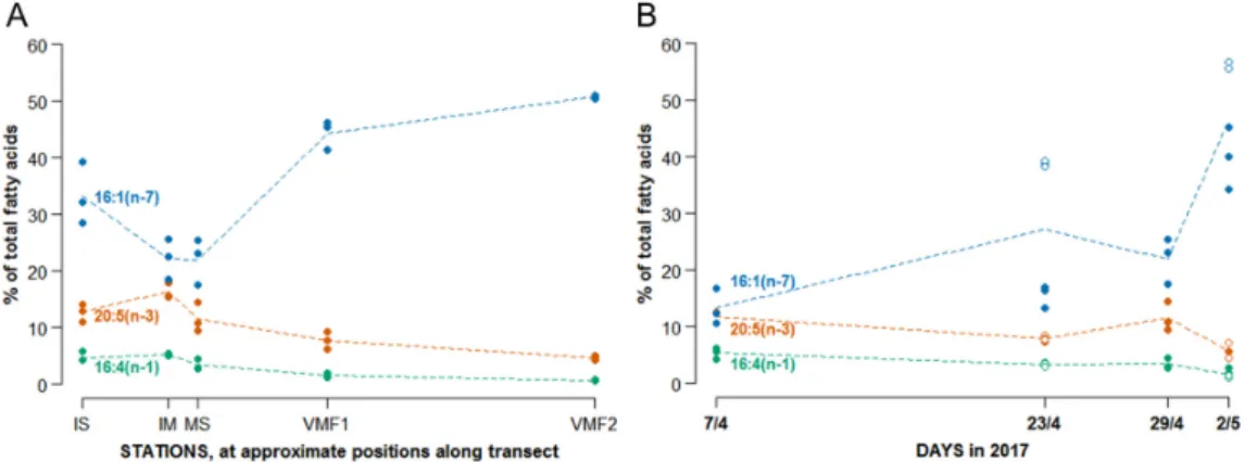
Diatom fatty acid markers (16:1(n-7), 16:4(n-1), and 20:5(n-3) were detected in all samples collected along the transect, but with different relative abundances. In communities collected in shallow areas close to shore, fatty acid composition consisted of 18% 20:5(n-3) and up to 6% 16:4(n-1), while samples collected at the mid-fjord stations VMF1 and VMF2 were characterized by almost 50% 16:1(n-7), and only 4.5–8% 20:5(n-3), and 0.7–1.6% 16:4(n-1) (Figure4A, Table S2). When summarizing all C16
J. Mar. Sci. Eng.2020,8, 676 11 of 24
PUFAs (a measure that is often used as a diatom indicator), a reduction by 80% was found between the shallowest and the deepest areas. Overall PUFAs were 50% lower at VMF1 compared to the innermost two stations (IS and IM), and about 66% lower at VMF2. Very similar changes in fatty acid composition were also found over time at MS station, with equally high percentages of 16:1(n-7) on the last sampling date (Figure4B). PUFAs decreased substantially over time, 20:5(n-3) accounting for up to 12% of all fatty acids in early April, but for only less than 6% in early May, and the corresponding values for 16:4(n-1) were 6 vs. 2% (Figure4B, Table S2).
J. Mar. Sci. Eng. 2020, 8, x FOR PEER REVIEW 11 of 25
3.3. Variability of Ice Algal Biomarkers on Short Spatial and Temporal Scales
All sea ice algal trophic markers displayed a remarkable variability along the sampling transect in the inner part of Van Mijenfjorden.
3.3.1. FATM
Diatom fatty acid markers (16:1(n-7), 16:4(n-1), and 20:5(n-3) were detected in all samples collected along the transect, but with different relative abundances. In communities collected in shallow areas close to shore, fatty acid composition consisted of 18% 20:5(n-3) and up to 6% 16:4(n- 1), while samples collected at the mid-fjord stations VMF1 and VMF2 were characterized by almost 50% 16:1(n-7), and only 4.5–8% 20:5(n-3), and 0.7–1.6% 16:4(n-1) (Figure 4A, Table S2). When summarizing all C16 PUFAs (a measure that is often used as a diatom indicator), a reduction by 80%
was found between the shallowest and the deepest areas. Overall PUFAs were 50% lower at VMF1 compared to the innermost two stations (IS and IM), and about 66% lower at VMF2. Very similar changes in fatty acid composition were also found over time at MS station, with equally high percentages of 16:1(n-7) on the last sampling date (Figure 4B). PUFAs decreased substantially over time, 20:5(n-3) accounting for up to 12% of all fatty acids in early April, but for only less than 6% in early May, and the corresponding values for 16:4(n-1) were 6 vs. 2% (Figure 4B, Table S2).
Figure 4. Relative abundances (%) of the most important diatom fatty acid trophic markers, 16:1(n-7), 16:4(n-1) and 20:5(n-3) along the transect (A), and measured at MS over time (B).
3.3.2. HBIs
Along the transect, highest values of the ice algae biomarker IP25 (normalized to POC) were detected at IM and MS station (on average 0.007–8 w/w), about 50% of these values at the shallowest station, and very little at mid-fjord stations VMF1 and VMF2 (Figure 5). Without normalization, the highest IP25 concentrations were found at the shallowest station IS with 50.5 pg mL−1, decreasing towards VMF2 where only 0.5 pg mL−1 was found (Table 1).
Figure 4.Relative abundances (%) of the most important diatom fatty acid trophic markers, 16:1(n-7), 16:4(n-1) and 20:5(n-3) along the transect (A), and measured at MS over time (B).
3.3.2. HBIs
Along the transect, highest values of the ice algae biomarker IP25(normalized to POC) were detected at IM and MS station (on average 0.007–8w/w), about 50% of these values at the shallowest station, and very little at mid-fjord stations VMF1 and VMF2 (Figure5). Without normalization, the highest IP25concentrations were found at the shallowest station IS with 50.5 pg mL−1, decreasing towards VMF2 where only 0.5 pg mLJ. Mar. Sci. Eng. 2020, 8, x FOR PEER REVIEW −1was found (Table1). 12 of 25
Figure 5. IP25 normalized to POC (w/w) along the transect (A) and changing over time at MS station (B). Open symbols depict low snow cover (less than 5 cm), filled symbols intermediate-high snow cover.
3.3.3. Stable Isotope Ratios
Stable isotope ratios in particulate organic carbon (δ13C POC) along the transect ranged from −23 to −22‰ at the shallowest near-shore stations to −19 to −18‰ at VMF1 and VMF2, respectively. For single diatom marker fatty acids, δ13C values were considerably higher (i.e., more enriched) at VMF2 than any other station, with some variability between the different fatty acids, but an overall consistent pattern (Figure 6A, Table S3). δ13C for 16:1(n-7), 16:0, and 20:5(n-3) were more enriched at VMF1 compared to MS, IM, and IS, whereas no such difference was found for δ13C 16:4(n-1). Stable isotope ratios of bulk POC measured over time at MS station were rather stable throughout April (21–23‰), with increasing (more enriched) δ13C values only on the very last day of sampling in early May (2/5), in particular at the site with little to no snow coverage (15‰, Figure 6B, Table S3).
Figure 6. δ13C for bulk POC (in black) and single diatom marker FAs (in color), determined along the transect (A), and measured at MS over time (B). Open symbols indicate sampling sites with very little snow cover (<5 cm), filled symbols sites with intermediate to high snow coverage.
3.4. Comparing the Ability of Different Markers to Distinguish Between Algae Collected in Sea Ice vs. Water Column
During sampling we observed the co-occurrence of a phytoplankton spring bloom that peaked almost simultaneously with the ice algal bloom in Van Mijenfjorden in late April/early May 2017 [44].
We used this opportunity to test whether it was possible to distinguish samples taken from the lowermost section of ice cores (0–3 cm) from those collected from different depths in the water Figure 5.IP25normalized to POC (w/w) along the transect (A) and changing over time at MS station (B).
Open symbols depict low snow cover (less than 5 cm), filled symbols intermediate-high snow cover.
3.3.3. Stable Isotope Ratios
Stable isotope ratios in particulate organic carbon (δ13C POC) along the transect ranged from
−23 to−22%at the shallowest near-shore stations to−19 to−18%at VMF1 and VMF2, respectively.
For single diatom marker fatty acids,δ13C values were considerably higher (i.e., more enriched) at VMF2 than any other station, with some variability between the different fatty acids, but an overall consistent pattern (Figure6A, Table S3). δ13C for 16:1(n-7), 16:0, and 20:5(n-3) were more enriched at VMF1 compared to MS, IM, and IS, whereas no such difference was found for δ13C 16:4(n-1).
Stable isotope ratios of bulk POC measured over time at MS station were rather stable throughout
J. Mar. Sci. Eng.2020,8, 676 12 of 24
April (21–23%), with increasing (more enriched)δ13C values only on the very last day of sampling in early May (2/5), in particular at the site with little to no snow coverage (15%, Figure6B, Table S3).
J. Mar. Sci. Eng. 2020, 8, x FOR PEER REVIEW 12 of 25
Figure 5. IP25 normalized to POC (w/w) along the transect (A) and changing over time at MS station (B). Open symbols depict low snow cover (less than 5 cm), filled symbols intermediate-high snow cover.
3.3.3. Stable Isotope Ratios
Stable isotope ratios in particulate organic carbon (δ13C POC) along the transect ranged from −23 to −22‰ at the shallowest near-shore stations to −19 to −18‰ at VMF1 and VMF2, respectively. For single diatom marker fatty acids, δ13C values were considerably higher (i.e., more enriched) at VMF2 than any other station, with some variability between the different fatty acids, but an overall consistent pattern (Figure 6A, Table S3). δ13C for 16:1(n-7), 16:0, and 20:5(n-3) were more enriched at VMF1 compared to MS, IM, and IS, whereas no such difference was found for δ13C 16:4(n-1). Stable isotope ratios of bulk POC measured over time at MS station were rather stable throughout April (21–23‰), with increasing (more enriched) δ13C values only on the very last day of sampling in early May (2/5), in particular at the site with little to no snow coverage (15‰, Figure 6B, Table S3).
Figure 6. δ13C for bulk POC (in black) and single diatom marker FAs (in color), determined along the transect (A), and measured at MS over time (B). Open symbols indicate sampling sites with very little snow cover (<5 cm), filled symbols sites with intermediate to high snow coverage.
3.4. Comparing the Ability of Different Markers to Distinguish Between Algae Collected in Sea Ice vs. Water Column
During sampling we observed the co-occurrence of a phytoplankton spring bloom that peaked almost simultaneously with the ice algal bloom in Van Mijenfjorden in late April/early May 2017 [44].
We used this opportunity to test whether it was possible to distinguish samples taken from the lowermost section of ice cores (0–3 cm) from those collected from different depths in the water Figure 6. δ13C for bulk POC (in black) and single diatom marker FAs (in color), determined along the transect (A), and measured at MS over time (B). Open symbols indicate sampling sites with very little snow cover (<5 cm), filled symbols sites with intermediate to high snow coverage.
3.4. Comparing the Ability of Different Markers to Distinguish between Algae Collected in Sea Ice vs. Water Column During sampling we observed the co-occurrence of a phytoplankton spring bloom that peaked almost simultaneously with the ice algal bloom in Van Mijenfjorden in late April/early May 2017 [44].
We used this opportunity to test whether it was possible to distinguish samples taken from the lowermost section of ice cores (0–3 cm) from those collected from different depths in the water column based on the lipid and stable isotope composition. To this end, we carried out a CCA where the first dimension was constrained to reflect the distinction between sea ice vs. water samples in the best possible way.
This was done separately for each biomarker approach; complete fatty acid composition (Figure7), HBIs (Figure8), and compound specificδ13C of individual fatty acids (Figure9).
J. Mar. Sci. Eng. 2020, 8, x FOR PEER REVIEW 13 of 25
column based on the lipid and stable isotope composition. To this end, we carried out a CCA where the first dimension was constrained to reflect the distinction between sea ice vs. water samples in the best possible way. This was done separately for each biomarker approach; complete fatty acid composition (Figure 7), HBIs (Figure 8), and compound specific δ13C of individual fatty acids (Figure 9).
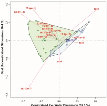
Distinction based on fatty acid composition resulted in a first constrained axis with very high explanatory power (65% of total variability), but did not yield a complete separation of samples within the first two dimensions, with a number of water column samples being grouped close to sea ice samples (Figure 7). Nonetheless, most of the sea ice samples had higher percentages of PUFAs than those from the water column. The HBI-based multivariate analyses yield a first axis with a similarly high explanatory power (63% of total variability) but, in contrast to FAs, provided a very clear and consistent distinction between sea ice and water samples (Figure 8) within the first two dimensions. Sea ice samples had relatively higher concentrations of sea ice diatom HBIs; IP25 as well as the HBIs IIb and IVc relative to samples of pelagic origin.When comparing all samples based only on the δ13C of individual fatty acids, the variability explained by the ice-water contrast on the first axis decreased to 11.2% of the total (Figure 9). This reflected the enormous variability of δ13C values within the sea ice samples which far exceeded the difference between pelagic and sea ice samples. In contrast, pelagic samples showed much less variability in their δ13C values.
Figure 7. Distinguishing particulate organic matter (POM) samples from Van Mijenfjorden (April 2017–May 2017) by means of their relative fatty acid composition (%), using a canonical correspondence analysis (CCA). Every dot represents a sample, green are samples from 0–3 sections of sea ice, in blue are samples taken from the water column.
Figure 7. Distinguishing particulate organic matter (POM) samples from Van Mijenfjorden (April 2017–May 2017) by means of their relative fatty acid composition (%), using a canonical correspondence analysis (CCA). Every dot represents a sample, green are samples from 0–3 sections of sea ice, in blue are samples taken from the water column.
J. Mar. Sci. Eng.2020,8, 676 13 of 24
J. Mar. Sci. Eng. 2020, 8, x FOR PEER REVIEW 14 of 25
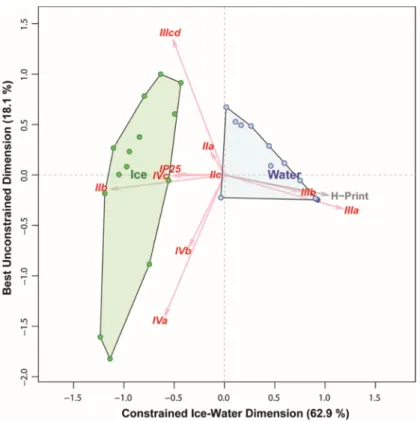
Figure 8. Distinguishing POM samples from Van Mijenfjorden (April 2017–May 2017) based on their HBI (highly branches isoprenoids) composition, using a CCA. Every dot represents a sample, green are samples from 0–3 sections of sea ice, in blue are samples taken from the water column.
Figure 9. Distinguishing POM samples from Van Mijenfjorden (April 2017–May 2017) based on δ13C of individual fatty acids, using an RDA. Every dot represents a sample, green are samples from 0–3 sections of sea ice, in blue are samples taken from the water column.
Figure 8.Distinguishing POM samples from Van Mijenfjorden (April 2017–May 2017) based on their HBI (highly branches isoprenoids) composition, using a CCA. Every dot represents a sample, green are samples from 0–3 sections of sea ice, in blue are samples taken from the water column.
J. Mar. Sci. Eng. 2020, 8, x FOR PEER REVIEW 14 of 25
Figure 8. Distinguishing POM samples from Van Mijenfjorden (April 2017–May 2017) based on their HBI (highly branches isoprenoids) composition, using a CCA. Every dot represents a sample, green are samples from 0–3 sections of sea ice, in blue are samples taken from the water column.
Figure 9. Distinguishing POM samples from Van Mijenfjorden (April 2017–May 2017) based on δ13C of individual fatty acids, using an RDA. Every dot represents a sample, green are samples from 0–3 sections of sea ice, in blue are samples taken from the water column.
Figure 9.Distinguishing POM samples from Van Mijenfjorden (April 2017–May 2017) based onδ13C of individual fatty acids, using an RDA. Every dot represents a sample, green are samples from 0–3 sections of sea ice, in blue are samples taken from the water column.
J. Mar. Sci. Eng.2020,8, 676 14 of 24
Distinction based on fatty acid composition resulted in a first constrained axis with very high explanatory power (65% of total variability), but did not yield a complete separation of samples within the first two dimensions, with a number of water column samples being grouped close to sea ice samples (Figure7). Nonetheless, most of the sea ice samples had higher percentages of PUFAs than those from the water column. The HBI-based multivariate analyses yield a first axis with a similarly high explanatory power (63% of total variability) but, in contrast to FAs, provided a very clear and consistent distinction between sea ice and water samples (Figure8) within the first two dimensions.
Sea ice samples had relatively higher concentrations of sea ice diatom HBIs; IP25as well as the HBIs IIb and IVc relative to samples of pelagic origin. When comparing all samples based only on theδ13C of individual fatty acids, the variability explained by the ice-water contrast on the first axis decreased to 11.2% of the total (Figure9). This reflected the enormous variability ofδ13C values within the sea ice samples which far exceeded the difference between pelagic and sea ice samples. In contrast, pelagic samples showed much less variability in theirδ13C values.
4. Discussion
4.1. Variability of Trophic Markers—And How This Relates to Environmental Conditions
Our results document a considerable variability in all studied trophic markers on short temporal and spatial scales. This is in line with previous findings (e.g., [17,28,30]), but we are, for the first time, able to show this systematically in a comparison including four different marker approaches in one dataset. In order to use trophic markers reliably and in a scientifically sound way, one needs to understand their biochemical nature and acknowledge the intrinsic coupling of growth conditions and physiological state of microalgae with their trophic marker baseline signal. It was remarkable to see how well the spatial variability of both nutrient concentrations and trophic markers resembled their changes over time: starting from early April (similar to the shallowest transect stations IS, IM) to early May (resembling VMF1 and VMF2, see Figures4–6). Hence, we conclude that at least one underlying factor explaining the spatial variability along the transect corresponds to a delay in bloom development at the shallowest stations. This is reflected in the replete nutrient concentrations at these stations. The lower dissolved inorganic carbon (DIC) concentrations at the outer stations relative to the inner one (MS) also indicated an earlier bloom start at the former (i.e., a further progressed bloom development at the time of sampling).
During bloom succession, several environmental parameters change simultaneously (e.g., availability of inorganic carbon and nutrients, light, temperature, etc.), and it is therefore impossible to completely disentangle their individual impact on trophic marker qualities from field observations only. However, our results point towards a key role of nutrient limitation that led to profound changes in trophic marker signals, as the samples that differ strongest from each other with respect to their fatty acid composition or their isotopic signal originate from samples with contrasting nutrient concentrations. Nutrient limitation is reflected in low absolute concentrations of the limiting nutrients in the water, but also, indirectly, in the stoichiometric ratios of POC:PON from particulate sympagic matter deviating from Redfield-ratios. We therefore analyzed the correlations of our trophic marker compounds with (a) nitrate concentrations, (b) silicate concentrations, and (c) C:N ratios of POM. In total, we found 11 significant or highly significant correlations, four of which were with nitrate concentrations, one with silicate (IP25normalized to POC), and six with C:N ratios (Table2). The only two markers tested that were not significantly correlated with any of these three parameters were the compound-specificδ13C values for the diatom PUFAs 16:4(n-1) and 20:5(n-3). The time series data of these two markers were also the ones hardly increasing at all (Figure6B), although they were found to be markedly different at station VMF2 compared to all other stations in the transect (Figure6A).
Unfortunately, we do not have complete datasets for all other environmental variables—and in particular DIC - whose impacts could have been tested in a similar manner, even though strong autocorrelation between some of them likely would complicated this type of analyses. But the highly significant

![Figure 10. Distinguishing pelagic and sympagic POM samples based on their fatty acid composition, using CCA: Example from Rijpfjorden 2007 (CLEOPATRA project, [16] and unpublished data)](https://thumb-eu.123doks.com/thumbv2/1library_info/5222624.1669809/19.892.253.646.129.522/figure-distinguishing-sympagic-composition-example-rijpfjorden-cleopatra-unpublished.webp)