How Marine Emissions of Bromoform Impact the
1
Remote Atmosphere
2 3
Yue Jia
1, Susann Tegtmeier
1, Elliot Atlas
2, Birgit Quack
14
5
1GEOMAR Helmholtz Centre for Ocean Research Kiel, Kiel, Germany
6
2University of Miami, 4600 Rickenbacker Causeway, Miami, USA
7 8
correspondence to: Yue Jia (yjia@geomar.de)
9
Abstract
10
Oceanic emissions of very short lived halocarbons (VSLH), such as CHBr3, are important for the halogen
11
budget of the atmosphere. It is an open question how localized elevated emissions in coastal and
12
upwelling regions and low background emissions, typically found over the open ocean, impact the
13
atmospheric VSLH distribution. In this study, we use the Lagrangian dispersion model FLEXPART to
14
simulate atmospheric CHBr3 resulting from uniform background emissions, on the one hand, and from
15
elevated emissions observed during three tropical cruise campaigns, on the other hand.
16
The simulations demonstrate that the atmospheric CHBr3 distributions due to uniform background
17
emissions are highly variable with accumulations taking place in regions of low wind speed. This relation
18
holds on regional and global scales demonstrating the importance of the atmospheric transport for the
19
distribution of short-lived trace gases with lifetimes in the range of days to weeks.
20
The impact of localized elevated emissions, measured during three research cruises, on the atmospheric
21
CHBr3 distribution varies significantly from campaign to campaign. The estimated impact depends on
22
the strength of the emissions and the meteorological conditions. In the open waters of the western Pacific
23
and Indian Ocean, localized elevated emissions only slightly increases the background concentrations of
24
atmospheric CHBr3, even when 1° wide source regions along the cruise tracks are assumed. Near the
25
coast, elevated emissions, including hotspots up to 100 times larger than the uniform background
26
emissions, can be strong enough to be distinguished from the atmospheric background. However, it is
27
not necessarily the highest hotspot emission that produces the largest enhancement, since the tug-of-war
28
between fast advective transport and local accumulation at the time of emission is also important.
29
Our analyses contribute to a better understanding and prediction of the timing and regional characteristics
30
of tropospheric CHBr3 distribution. Significantly, our results demonstrate that transport variations of the
31
atmosphere itself are sufficient to produce highly variable VSLH distributions, and elevated VSLH in
32
the atmosphere do not always reflect a strong localized source. Localized elevated emissions can be
33
obliterated by the highly variable atmospheric background, even if they are orders of magnitude larger
34
than the average open ocean emissions.
35
36
1. Introduction
37 38
Very short lived halocarbons (VSLHs) with atmospheric lifetimes shorter than 6 months have natural
39
oceanic sources which are dominated by brominated and iodinated compounds (Carpenter and Liss, 2000;
40
Quack et al., 2004; Law et al., 2006). VSLHs have drawn considerable interest due to their contribution
41
to stratospheric ozone depletion and tropospheric chemistry (Solomon et al., 1994; Dvortsov et al., 1999;
42
Salawitch et al., 2005; Feng et al., 2007; Tegtmeier et al., 2015; Hossaini et al., 2015). In this work, we
43
focus on the VSLH bromoform (CHBr3), since most organic oceanic bromine is released into the
44
atmosphere in this form.
45
CHBr3 concentrations measured in ocean waters are characterized by large spatial variability with
46
elevated abundances in phytoplankton blooms (Baker et al., 2000, Liu et al., 2013) and equatorial and
47
upwelling regions due to biological sources (Carpenter et al., 2009; Quack and Wallace, 2003; Quack et
48
al., 2007; Fuhlbrügge et al., 2016). The open ocean generally shows quite homogeneous, low CHBr3
49
concentrations, compared to higher concentrations and strong gradients found in coastal and shelf areas
50
(Quack and Wallace, 2003), At the coast, high oceanic concentrations are related to macro algae (Klick
51
and Abrahamsson, 1992) and anthropogenic sources (Boudjellaba et al., 2016) such as power plants
52
(Yang, 2001) and desalination facilities (Agus et al., 2009).
53
Due to sparse measurements and limited process understanding, existing estimates of global air-sea flux
54
distributions of CHBr3 and other VSLHs are subject to large uncertainties (e.g. Warwick et al., 2006;
55
Palmer and Reason, 2009; Liang et al., 2010; Ordóñez et al., 2012; Stemmler et al., 2013; Ziska et al.,
56
2013; Carpenter et al., 2014). Open ocean background emissions of CHBr3 are modeled to be around
57
100 pmol m-2 hr-1 (Ziska et al., 2013), consistent with simultaneous in-situ measurements of air and water
58
concentrations (Butler et al., 2007; Liu et al., 2013; Fiehn et al., 2017). The spatial and temporal
59
distribution of elevated emissions in coastal and upwelling regions is currently based on very limited
60
observations. Campaigns in these regions suggest that emissions generally increase near coastlines, and
61
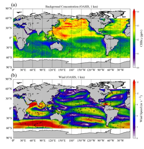
that sporadic peak emissions with extremely high values can be found (e.g. Butler et al., 2007; Liu et al.,
62
2013; Fuhlbrügge et al., 2016; Fiehn et al., 2017). Analysis of the measurements suggests that such peak
63
emissions are often of limited spatial extent and cover not more than a distance of 50-100 km along the
64
cruise track. We will use the term ‘elevated emissions’ when describing emissions that are on average
65
up to a factor of 10 larger than the background and ‘hotspot emissions’ for sporadic emissions up to a
66
factor of 100 larger than the background.
67
There are two main approaches to derive the magnitude of VSLH emissions, i.e. “bottom-up” approach
68
(e.g. Quack and Wallace, 2003; Carpenter and Liss, 2000; Butler et al., 2007; Ziska et al., 2013) and
69
“top-down” approach (e.g. Warwick et al., 2006; Liang et al., 2010; Ordóñez et al., 2012). For the
70
“bottom-up” method, measured surface sea water concentrations of VSLHs at the “bottom” (surface) are
71
extrapolated to estimate global emissions. For the “top-down” method, the emissions of VSLHs are
72
constrained by the measured abundances at the “top” (atmosphere) so that model simulations based on
73
the constrained global emission estimates reproduce the observed atmospheric concentrations. These two
74
approaches yield different estimates of the global VSLHs emissions, with the recent “top-down”
75
approaches resulting in generally higher emissions than the recent “bottom-up” approaches.
76
In the tropical ocean waters of the Atlantic, the western Pacific and Indian Ocean, the existence of
77
localized elevated CHBr3 emissions and hotspots has been confirmed (Butler, et al, 2007; Liu et al., 2013;
78
Krüger and Quack, 2013; Quack and Krüger, 2013; Fiehn et al., 2017). At the same time, these
79
convectively active regions offer an efficient pathway for the vertical transport of short-lived oceanic
80
compounds from the boundary layer to the stratosphere (e.g. Aschmann et al., 2009; Hossaini et al., 2012;
81
Tegtmeier et al., 2012, 2013; Marandino et al., 2013; Liang et al., 2014). Moreover, the Asian monsoon
82
has been recognized as an efficient transport pathway for short-lived pollutants and VSLHs (Randel et
83
al., 2010; Hossaini et al., 2016; Fiehn et al., 2017). Given that elevated oceanic CHBr3 emissions are
84
expected to occur in the same regions as strong convection, it is of interest to analyze how these elevated
85
emissions impact CHBr3 in the atmospheric boundary layer, which feeds into the upward transport.
86
Measurements of CHBr3 abundance in the atmospheric boundary layer show large spatial variability (e.g.,
87
Quack and Wallace, 2003; Montzka and Reimann, 2011; Lennartz et al., 2017). A compilation of
88
available measurements by Ziska et al. (2013) suggests similar CHBr3 distribution patterns in the
89
atmospheric boundary layer as in the surface ocean, with higher mixing ratios in the equatorial, coastal
90
and upwelling regions. However, given the sparse data base and the uncertainties in the spatial and
91
temporal extent of oceanic emissions, the detailed distribution of boundary layer CHBr3, cannot be well
92
constrained (e.g., Hepach et al., 2014; Fuhlbrügge, et al., 2013). On the one hand, the spatial and temporal
93
extent of elevated localized emissions is usually unknown, leading to large uncertainties when estimating
94
their overall magnitudes. On the other hand, the influence of meteorological conditions, distinctive
95
transport patterns and variations of atmospheric sinks, such as the background OH field (e.g. Rex et al.,
96
2014), can be expected to modulate the effect of elevated oceanic sources. Therefore, it is still an open
97
question of the magnitude of elevated and hotspot emissions on the local atmospheric CHBr3 distribution.
98
Such knowledge is relevant to understand the importance of localized elevated emissions for atmospheric
99
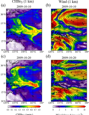
abundances and to interpret existing atmospheric measurements with respect to potential sources and
100
driving factors.
101
In this study, we use observational data from three tropical research cruises, one in the Indian Ocean
102
(OASIS) and two in the western Pacific (TransBrom and SHIVA). We use the Lagrangian particle
103
dispersion model FLEXPART to investigate the transport and atmospheric distribution of VSLHs.
104
Taking bromoform (CHBr3) as example, we compare the atmospheric signals estimated from the elevated
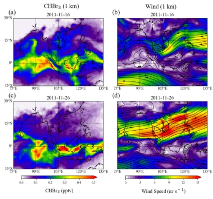
105
and hotspot emissions measured during the ship campaigns to the distribution derived from only uniform
106
background emissions. The campaigns and the FLEXPART model are introduced in Sect. 2. In Section
107
3, we discuss the distributions and variability of atmospheric CHBr3 based on uniform background
108
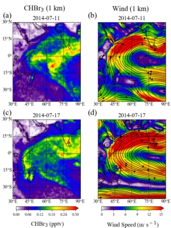
emissions. We present the observed hotspots of CHBr3 emissions in Section 4.1, and compare the
109
simulated atmospheric mixing ratios resulting from elevated emissions during three campaigns with the
110
background values (Section 4.2). Conclusions are given in Section 5.
111 112
2. Data and Methods
113 114
2.1 Background and in-situ CHBr3 emissions
115 116
In this study, we distinguish between open ocean background and in-situ CHBr3 emissions. Open ocean
117
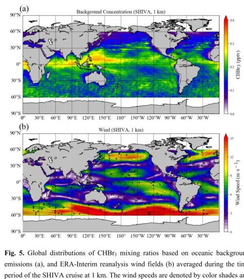
emissions are deduced to be around 100 pmol h-1 m-2 based on global bottom up scenarios (Quack and
118
Wallace, 2003, Ziska et al., 2013). While emissions for individual regions and seasons can be higher or
119
lower than this, including negative fluxes going from the atmosphere into the ocean, 100 pmol h-1 m-2
120
represents the typical mean value averaged over all oceanic basins between 60°S and 60°N. The
121
background open ocean emissions exclude by design emissions from coastal, shelf and upwelling regions.
122 123
In-situ oceanic emissions of CHBr3 have been calculated from the observational data collected during
124
three tropical ship campaigns. The two campaigns TransBrom (October 11th-23rd, 2009, Krüger and
125
Quack, 2013) and SHIVA (November 15th-28th, 2011, Quack and Krüger, 2013) took place in the
126
western Pacific, while the OASIS campaign (July 11th-August 6th, 2014, Fiehn et al., 2017) was
127
conducted in the western Indian Ocean. During each campaign, surface air and water samples were
128
collected simultaneously at regular intervals (every 3 to 6 hours). The emissions were calculated from
129
these co-located data and the instantaneous wind speed (Ziska et al., 2013, Fuhlbrügge et al., 2016, Fiehn
130
et al., 2017). The detailed cruise track and the magnitude of the oceanic CHBr3 emissions of each
131
campaign is given in Fig. 1. The in-situ emissions include both open-ocean emissions and elevated
132
emissions from coastal, shelf and upwelling regions with our evaluations focusing on the regions of
133
elevated emission.
134 135
2.2 Modeling
136 137
For the simulations of the atmospheric distribution and transport of CHBr3, we used the Lagrangian
138
particle dispersion model, FLEXPART (Stohl et al., 2005), which has been validated by previous
139
comparisons with measurements (Stohl et al., 1998; Stohl and Trickl, 1999). Lagrangian particle models
140
such as FLEXPART compute trajectories of a large number of so-called particles, presenting
141
infinitesimally small air parcels, to describe the transport, diffusion and chemical decay of tracers in the
142
atmosphere. The model includes turbulence in the boundary layer and free troposphere (Stohl and
143
Thomson, 1999) and a moist convection scheme (Forster et al., 2007) following the parameterization by
144
Emanuel and Živković-Rothman (1999). The representation of convection in FLEXPART simulations
145
has been validated with tracer experiments and 222Rn measurements (Forster et al., 2007). Chemical or
146
radioactive decay of the transported tracer is accounted for by reducing the particle mass according to a
147
prescribed lifetime of the tracer. Alternatively, the loss processes can be prescribed via OH reaction
148
based on a monthly averaged 3 dimensional OH-field. In this study, we employ FLEXPART version
149
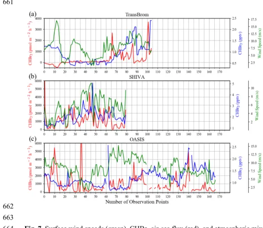
10.0, which is driven by 3-hourly meteorological fields from ECMWF (European Centre for Medium-
150
Range Weather Forecasts) reanalysis product ERA-Interim (Dee et al., 2011) with a horizontal resolution
151
of 1º x 1º and 61 vertical model levels.
152
We performed two kinds of simulations based on the different emission scenarios. The first one used the
153
uniform global background emission, and the second one used in situ emissions observed during
154
individual ship campaigns. Chemical decay of CHBr3 was simulated by prescribing a lifetime of 17 days
155
during all runs (Montzka and Reimann, 2011). For the background runs, a uniform air-sea flux of 100
156
pmol h-1 m-2 is prescribed over all ocean surface area between 60°S and 60°N. Three runs are conducted
157
covering the time period of the campaigns with a 1-month spin-up period in each case to reach a stable
158
background concentration in the atmosphere.
159
For the in-situ emissions of each campaign, simulations are based on the calculated CHBr3 air-sea flux
160
(see Fig. 7, detailed description in Sec 4), which is released along the cruise track. The periods of these
161
campaign simulations are the same as the corresponding background simulations with emissions over
162
the whole time period. For each observational data point, an emission grid cell centered on the
163
measurement location is created. These grid cells are designed to be adjacent along the cruise track and,
164
based on the density of the measurements, are about 0.1 – 2.0° wide in cruise track direction. The grid
165
cells are chosen to be of a fixed width (0.5° or 1°) in the other direction and thus add up to the narrow
166
band of 0.5° or 1° width centered along the cruise track (Fig. 1). Our design of the emission grid cells
167
assumes that the elevated emissions can extend over a distance of 0.5°-1°. This choice has been motivated
168
by the spatial variability of the measurements along the cruise track (see also section 4.1 and Fig. 7).
169
Elevated emissions larger than 1000 pmol h-1 m-2 are found at 77 different locations along the three cruise
170
tracks examined in this paper. Out of the 77 measurements, only 11 correspond to singular locations with
171
no adjacent high emissions at the neighboring points. The other 66 measurements cluster together at 18
172
different locations with at least two adjacent observational points showing emissions larger than 1000
173
pmol h-1 m-2. We define the length of such a location of elevated emissions as the distance between the
174
first and last data point with an air-sea flux exceeding 1000 pmol h-1 m-2. Most of the 18 locations extent
175
over a distance larger than 0.5° (13 out of 18) and nearly half are larger than 1° (8 out of 18) supporting
176
our choice of the width of the emissions grid cells. Note that at the same time, the spatial extent of the
177
hotspots is comparable to the wind field resolution that drive our trajectory simulations. The amount of
178
CHBr3 released from each grid cell is determined by the observational air-sea flux of the corresponding
179
data point and scales with the width of the narrow emission band described above.The specified CHBr3
180
emission from each cell is kept constant for the duration of the model run and distributed over a fixed
181
number of trajectories. In order to capture the small scale processes (e.g. convection), the large number
182
of 2000, and 20000 trajectories are chosen to be released from each emission grid cell of background run
183
and in-situ run, respectively. Output data in form of CHBr3 volume mixing ratios available at a user-
184
defined grid, is retrieved at a horizontal resolution of 1º x 1º and 0.5º x 0.5º for background runs and in-
185
situ runs, respectively, at every 100 m from 100 m to 1 km, and every 1 km from 1 km to 20 km every 3
186
hours.
187 188
3. Atmospheric CHBr3 based on open ocean background emissions
189 190
The atmospheric CHBr3 mixing ratios diagnosed from the uniform background emissions (referred to as
191
CHBr3 background mixing ratios hereinafter) vary significantly from campaign to campaign and also
192
within each campaign region. Figures 2 to 4 present several snapshots of the CHBr3 background mixing
193
ratios and the simultaneous wind fields from ERA-Interim reanalysis for the three campaigns. For
194
TransBrom (Fig. 2), CHBr3 accumulates south of 15º N with a maximum near the equator, where the
195
wind is weak. In the northern Pacific, which was dominated by an anticyclone centered around 165°E,
196
30°N, the background values are much lower. On the 10th of October 2009, two bands of extremely low
197
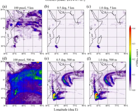
wind fields exist, one directly south of the equator and one tilting from 15°N to 5°N, which both coincide
198
with the highest CHBr3 abundances. On the 20th of October, these two bands collided into one with
199
lowest winds centered around 165°E, where we again find very high values of CHBr3 of up to 0.8 ppt.
200
For both case studies, highest values are found in the region of the lowest wind speeds or slightly shifted
201
towards the region of strongest wind shear. Regions of high wind speeds, such as the northern Pacific
202
anticyclone, on the other hand do not allow for accumulations and are characterized by very low CHBr3.
203
For the SHIVA case (Fig. 3), the background CHBr3 accumulates in a narrow region near Indonesia,
204
with corresponding wind fields smaller than 3 m/s. North of Indonesia, the strong easterly trade winds
205
generally above 10 m/s prevent the accumulation of higher background values within the region. Again,
206
the two case studies illustrate how changes of the wind patterns within a few days drive changes of the
207
background CHBr3 distribution. Another particular example is the northward extension of the low
208
equatorial winds around 90°E on 16th November 2011, which leads to higher CHBr3 north of the equator
209
up to 15°N.
210
For OASIS (Fig. 4), the wind speed is higher than in the other two regions and these strong
211
southeast/southwest trade winds associated with the Asian monsoon extend over most of the Indian
212
Ocean. Consistent with the stronger winds, the background values for the OASIS case are significantly
213
lower than for the other two cases, although they also show accumulations in certain regions. These
214
accumulations appear partially in regions of low wind speeds (e.g., near the equator between 70°E and
215
90°E on 17th of July) or in adjacent regions of high wind shear (e.g., north of the equator between 70°E
216
and 90°E for both case studies). For the latter case, the CHBr3 accumulation also extends into the region
217
of high wind speeds, which is different from the distribution found for the TransBrom and SHIVA
218
regions. This difference occurs because the east coast of the Indian Subcontinent offshore is a region
219
with wind convergence (not shown), which tends to accumulate air masses therein.
220
Given that the accumulation of CHBr3 background mixing ratios follows in most cases the wind field
221
patterns on a regional scale, we hypothesize that the same relationship holds on a global scale. The global
222
distributions of atmospheric CHBr3 based on background emissions and wind fields averaged over the
223
time periods of the SHIVA and OASIS cruise are presented in Fig. 5 and 6, respectively. We omit the
224
time period of the TransBrom case, since the background CHBr3 distribution diagnosed for this period
225
is very similar to background found for the SHIVA period. The global CHBr3 background mixing ratios
226
(Fig. 5a, and 6a) display a very heterogeneous distribution in spite of the uniform background emission
227
used for the simulations. Accumulations of CHBr3 are again generally located in the regions of low wind
228
speeds. For the SHIVA period (November 2011), particularly high CHBr3 background values of 0.3 to
229
0.4 ppt are found along the equator over the Maritime continent, West Pacific, Indian Ocean and at the
230
West coast of Africa, all of which are characterized by particularly low winds. In the Northern and
231
Southeast Pacific, the wind speed is generally higher, and the corresponding CHBr3 values of less than
232
0.15 ppt are much lower than in the tropical region. For the OASIS period (July/August 2014), the global
233
CHBr3 distribution is mostly reversed compared to the SHIVA period and high winds over the Indian
234
Ocean and Maritime continent lead to low CHBr3 abundance in this region. The North Pacific on the
235
other hand, with low wind speeds is now a region of intense accumulation leading to 0.3-0.4 ppt of CHBr3.
236
The tropical West Pacific is the only region that experiences relatively low winds during both seasons,
237
and constantly shows high CHBr3 for the SHIVA and OASIS time periods.
238
The variations of the background CHBr3 distribution can be generally explained by the seasonal
239
variations of the global wind field. The North Pacific and Northern Indian Ocean are dominated by the
240
East Asia Monsoon and the Monsoon of South Asia, respectively. The East Asia Monsoon is
241
characterized by strong northwesterly flow in boreal winter and weak southeasterly flow in boreal
242
summer due to the reverse of the thermal gradient between land and ocean (Webster, 1987; Ding and
243
Chan, 2005). Therefore, the accumulations of CHBr3 in the North Pacific occurs during the boreal
244
summer months, rather than during boreal autumn/ early winter (TransBrom time period). The Monsoon
245
of South Asia, on the other hand, is characterized by weak northeasterly winds in boreal winter and
246
strong southwesterly winds in boreal summer (Webster, 1987; Webster et al., 1998). Thus background
247
CHBr3 accumulation over the Northern Indian Ocean occurs mostly during boreal winter, while during
248
boreal summer (OASIS time period) a low CHBr3 background can be expected. Because of the light
249
winds of the Inter Tropical Convergence Zone (ITCZ), a belt of relatively high CHBr3 abundance exists
250
along the equator in the Northern Hemisphere, especially in the tropical Pacific and Atlantic. Strong
251
convection in the ITCZ enhances vertical transport of CHBr3 out of the boundary layer, but overall the
252
CHBr3 distribution is dominated by the horizontal wind fields and accompanying transport patterns. Due
253
to the more complex land-sea thermal difference, the seasonal variation of ITCZ in the West Pacific is
254
more significant than in the East Pacific (Waliser and Jiang, 2014). The relatively high accumulations of
255
CHBr3 in the tropical East Pacific are confined to a narrow region near the equator for both seasons. As
256
for the tropical West Pacific, during boreal winter the ITCZ covers almost the whole Southeast Asia and
257
the high CHBr3 abundances during SHIVA appear along the east coast of Malaysia. During boreal
258
summer, the ITCZ shifts northward and the high CHBr3 abundances retreat northwestward.
259
We assume constant CHBr3 open ocean emissions of 100 pmol h-1 m-2 for our simulations in order to
260
isolate the impact on the atmospheric CHBr3 distribution of atmospheric transport patterns versus the
261
impact of varying emission fields. In particular, variations of the wind fields will impact the ocean air-
262
sea flux, and emissions larger than 100 pmol h-1 m-2 might occur in regions of higher winds with little
263
CHBr3 accumulation. Such variations can change the background CHBr3 distribution and may allow for
264
increased mixing ratios in regions of strong winds. In addition to the wind speed, variations in the
265
atmospheric and, more importantly, the oceanic CHBr3 concentrations can impact the emission strength
266
which can further change the complex atmospheric CHBr3 distribution.
267 268
4. Atmospheric CHBr3 based on hotspot emissions
269 270
Given the high variability of the atmospheric CHBr3 background mixing ratios, resulting from
271
atmospheric transport processes (Section 3), it is of interest to analyze if and how much oceanic hotspot
272
emissions might impact this background distribution. In this section, we will use observational data to
273
discuss if oceanic hotspot emissions occur at the same time and location as peak atmospheric mixing
274
ratios or if the two quantities are rather uncorrelated. Furthermore, we will use FLEXPART simulations
275
to compare CHBr3 mixing ratios that result from background emissions to the increased CHBr3 mixing
276
ratios that result from localized hotspot emissions.
277 278
4.1 Observed hotspot emission
279 280
Oceanic CHBr3 emissions, atmospheric CHBr3 mixing ratios and the observed local surface wind speeds
281
are given in Fig. 7 for all three campaigns. The oceanic emissions of CHBr3 vary substantially from
282
campaign to campaign with mean values of 261 pmol h-1 m-2 (TransBrom), 1228 pmol h-1 m-2 (SHIVA),
283
and 912 pmol h-1 m-2 (OASIS) with standard deviations of 600 pmol h-1 m-2 (TransBrom), 1460 pmol h-1
284
m-2 (SHIVA) and 1159 pmol h-1 m-2 (OASIS), respectively. All three campaigns show periods with
285
background emissions around 100 pmol h-1 m-2 and periods with localized elevated and hotspot emissions.
286
For TransBrom, the first two thirds of the campaign show negative (air-to-sea) or very low background
287
CHBr3 fluxes, while the last third was close to western Pacific islands and is characterized by overall
288
elevated emissions with sporadic hotspots of up to 4000 pmol h-1 m-2. The SHIVA cruise track, on the
289
other hand, was mostly along the coastline, and low background emissions occur only for brief periods.
290
Most locations showed elevated emissions and hotspots occurred regularly. The OASIS cruise track
291
alternated between open ocean, upwelling and coastal areas, resulting in a large fluctuation between low
292
background and localized elevated emissions. Hotspot emissions during this campaign are largest,
293
reaching values of over 6000 pmol h-1 m-2.
294
According to the flux parameterization applied here, the air-sea flux is determined mostly by the surface
295
wind speed and the ocean-atmosphere concentration gradient. Highest emissions are expected to occur
296
during periods of high wind speed and large concentration gradients. The wind speed dominates the
297
fluxes for some regions, but not for entire campaigns. During the beginning of the TransBrom campaign
298
(Fig. 7a), the wind speed peaks at over 15m/sec while the corresponding CHBr3 air-sea flux is low.
299
Higher wind speeds co-occur with high air-sea fluxes at the end of the campaign. For SHIVA (Fig. 7b)
300
and OASIS (Fig. 7c), the relation between wind speed and CHBr3 emissions is more easily discernable.
301
All three campaigns demonstrate that high fluxes do not always lead to local high CHBr3 mixing ratios
302
in the surface atmosphere. For example, several hotspots with oceanic emissions over 4000 pmol m-2 hr-
303
1 are found during OASIS, however, corresponding atmospheric mixing ratios are relatively low (~ 2
304
ppt). Vice versa, the highest atmospheric mixing ratios found during OASIS do not coincide with high
305
fluxes, except for the last part of the campaign. These discrepancies suggest that the local atmospheric
306
mixing ratios are driven by a complex interplay of source and loss processes driving the atmospheric
307
mixing ratios of short-lived compounds. A relatively clear connection between elevated oceanic
308
emissions and surface mixing ratios only occurs during the SHIVA campaign and during the last part of
309
the TransBrom campaign (Fig 7a and b).
310
As the campaign data shows a relation between emissions and atmospheric mixing ratios only for some
311
regions, the question arises how much of the atmospheric variability of short-lived compounds such as
312
CHBr3 is impacted bythe emission strengths. In order to quantify the relative contributions of elevated
313
emissions, comparisons between the computed mixing ratios over hotspots and the background
314
abundances in the atmosphere are required. In the subsequent section, we present such comparisons based
315
on the model results.
316 317
4.2 Comparison of CHBr3 from background and hotspot emissions
318 319
In this section, we will compare the concentrations of CHBr3 due to background and localized elevated
320
emissions as simulated by FLEXPART. First, atmospheric CHBr3 during all three campaigns is
321
calculated based on the uniform background emission of 100 pmol h-1 m-2. Second, atmospheric CHBr3
322
resulting from strong localized emissions is simulated for the three case studies given by the campaigns.
323
Atmospheric CHBr3 at different altitudes is simulated by FLEXPART, which is driven by the
324
meteorological data from ECMWF. The signatures of dynamical processes such as wind regimes,
325
weather phenomena (e.g., typhoons) and convection are captured by the model simulation and can be
326
detected in the CHBr3 distribution (Fig. 8). For example, during the TransBrom campaign, the cruise
327
encountered several tropical storms in the western Pacific, one of which (Lupit, around October 14th,
328
2009) developed into a super typhoon within several days (Krüger and Quack, 2013). As shown in Fig.
329
8, an elevated CHBr3 accumulation representing the structure of typhoon Lupit is clearly visible in the
330
background distribution of CHBr3 at 500 m (Fig. 8d) altitude in the northern part of the western Pacific.
331
This structure is still clear at 5 km altitude (Fig. 8a), although with a weaker magnitude. For CHBr3
332
emitted from localized elevated sources (Figures 8b, c, e, and f), such large scale structures are not
333
discernible due to the small spatial extent of the 0.5° or 1° emission cells and thus the limited amount of
334
overall released CHBr3. A clear blob of higher abundances of atmospheric CHBr3 can be seen in the
335
southern part of the western Pacific near Indonesia resulting from one of the hotspot emissions observed
336
during TransBrom (Fig. 1b). However, the background CHBr3 in this area is also high in this low-wind
337
area, and thus the atmospheric signal of the up to 20 times stronger hotspot emissions (Fig. 7a) is
338
detectable for neither the 0.5° nor the 1° wide emission cells when compared to the background. Note
339
that the modelled atmospheric mixing ratios from both sources, hotspot and background emissions, are
340
smaller than the mixing ratios observed along the cruise track (Figure 7) suggesting stronger nearby
341
emissions not covered in our scenarios and observations. The signature of the hotspot emissions remains
342
in the boundary layer and cannot be seen at 5 km altitude.
343
Fig. 9 shows the atmospheric CHBr3 mixing ratios during the SHIVA campaign. For the SHIVA case,
344
the distribution patterns of the background CHBr3 abundances at 500 m altitude also show a very strong
345
spatial variability, despite the uniform emissions. Highest CHBr3 background mixing ratios around 120º
346
E near the equator of up to 0.5 ppt are smaller than background values found during TransBrom of up to
347
0.8 ppt. The atmospheric signal of the localized elevated emissions is much stronger than during
348
TransBrom due to stronger emissions on the one hand and smaller background mixing ratios on the other
349
hand. First, for the 0.5° wide emission grids, two highly localized, atmospheric CHBr3 peaks appear
350
close to the coast line near the equator around 105º E with a maximum value around 0.4 ppt. These
351
signals occur in a spot where the background is very low (0.2 ppt). However, at the same time they are
352
smaller than the maximum background values of up to 0.5 ppt in nearby regions (Fig. 9d). If the width
353
of the emission grids is extended to 1°, the localized CHBr3 peaks mentioned above grow into two distinct
354
blobs near the equator of up to 0.8 ppt. These maxima along the first half of the cruise track are apparently
355
larger than the regional background concentrations (Fig. 9f). Elevated emissions during the second half
356
of the campaign with several hotspot events, on the other hand, do not show such clear atmospheric
357
signals right above.
358
At 5 km altitude, the overall background values are slightly lower, but the maximum mixing ratios are
359
still comparable to altitudes below due to the intense convection in the general region of the SHIVA
360
campaign (Fuhlbrügge et al., 2016). For the regions of localized elevated emissions, the convection is
361
less effective and maximum mixing ratios at 5 km are about 50% smaller compared to the values in the
362
boundary layer. Krystofiak et al. (2018) calculated the fractions of convective-contributed trace gases
363
from boundary layer to the upper troposphere using airborne measurements during the SHIVA campaign
364
and reported an even smaller fraction of boundary layer CHBr3 in the upper troposphere (about 15% due
365
to convection). Thus only the signal of the 1° wide emission cells can be detected at 5 km, while assuming
366
that the emissions cover a smaller region of 0.5° width will render their impact in the free troposphere
367
negligible.
368
Due to the dominant southwest monsoon over the Northern Indian Ocean in boreal summer, the resulting
369
atmospheric abundances of the OASIS case (Fig. 10) for both scenarios, background and localized
370
emissions, are much lower than for the other two campaigns. This is particularly surprising for the OASIS
371
hotspot emissions, which are in many cases larger than hotspot emissions during TransBrom or SHIVA.
372
In the open ocean, the atmospheric enhanced CHBr3 mixing ratios resulting from the 0.5° (1°) wide
373
localized emission runs reach only 0.1 (0.2) ppt in a narrow belt near 60°E and are mostly smaller than
374
the background (around 0.15 ppt). An exception occurs near the coast of Madagascar, where both
375
background and hotspot emissions accumulate in the atmosphere. Maximum background values reach
376
up to 0.25 ppt and the hotspot signals peak with values of 0.3 ppt (0.5° wide emission cells) to 0.6 ppt
377
(1° wide emissions cells). These clear atmospheric signals of hotspot emissions are driven by the
378
enhanced coastal emissions near Madagascar. At 5 km altitude, atmospheric background values are very
379
low, and the hotspot contributions are close to zero.
380
In summary, the observed emissions during the three cruises were significantly higher than the
381
background of 100 pmol m-2 hr-1. Our results show that such strong oceanic sources are not necessarily
382
detectable in the atmosphere, where transport processes can sometimes mask the impact of oceanic
383
emissions on the atmospheric CHBr3 distribution.
384 385
5. Summary and Discussion
386 387
In this study, we simulated atmospheric CHBr3 abundances that result from uniform marine background
388
emissions compared to hotspot emissions using the Lagrangian dispersion model FLEXPART.
389
The simulations demonstrate that uniform background emissions from the ocean result in a highly
390
variable atmospheric CHBr3 distribution with accumulations taking place in regions of low wind speed.
391
This relation holds on regional and global scales revealing atmospheric transport processes as important
392
drivers of the distribution of short-lived trace gases with lifetimes in the range of days to weeks. The
393
relation between atmospheric background and wind patterns described here will allow us to better predict
394
the seasonal and regional characteristics of the tropospheric CHBr3 distribution. Such knowledge will
395
provide valuable information for analyzing and interpreting atmospheric data from ship and aircraft
396
campaigns. For example, our results illustrate that low atmospheric CHBr3 abundances cannot
397
necessarily be used to draw conclusions about the oceanic source strength below.
398
Comparisons between atmospheric CHBr3 resulting from background and peak emissions suggest that
399
the impact of localized elevated emission on the atmospheric CHBr3 distribution depends on their relative
400
strength, on their location and on the time of emission. The “visibility” of elevated emissions in the
401
atmospheric CHBr3 distribution varies significantly between three cruises in the West Pacific and Indian
402
Ocean. In the open ocean, signals of elevated emissions can hardly be distinguished from the background
403
CHBr3 distribution even for elevated sources extending over 1° wide source regions along the cruise
404
tracks. Near the coast, however, signals of elevated emissions are often strong enough to be distinguished
405
from the background. In particular, some of the hotspot emissions up to 100 times larger than the
406
background can be detected in the atmosphere. However, individual cases show that it is not necessarily
407
the largest hotspot that gives a clear signal, but that the tug of war between fast advective transport and
408
local accumulation at the time of emission is also important.
409
The constant background emissions of 100 pmol m-2 hr-1 used in our study are based on a simplified
410
scenario and do not take coastal and upwelling maxima into account. Realistic oceanic emissions are
411
much more complex with large gradients in the above mentioned regions. Nevertheless, our results
412
demonstrate that atmospheric CHBr3 signals, produced by localized elevated and even hotspot emissions,
413
orders of magnitudes larger than the average open ocean emissions, can be obliterated by the highly
414
variable atmospheric background. That is to say that transport variations of the atmosphere itself are
415
sufficient to produce high concentrations in certain regions and that high concentrations of VSLH in the
416
atmosphere do not always guarantee a strong local or regional source. For observational and modelling
417
studies of VSLS and other short-lived compounds, the impact of atmospheric transport patterns that are
418
identified here can be used for the interpretation of trace gas distributions and variability.
419
Data availability
420
The emission data of cruise campaigns are available at Pangaea (http://www.pangaea.de). FLEXPART
421
output can be inquired from the authors.
422 423
Author contribution
424
Y. Jia, S. Tegtmeier designed the model experiments. Y. Jia carried out the FLEXPART calculations and
425
produced the figures. Y. Jia and S. Tegtmeier wrote the manuscript with contributions from all co-authors.
426 427
Competing interests
428
The authors declare that they have no conflict of interest.
429 430
Acknowledgements
431
The authors would like to thank the European Centre for Medium-Range Weather Forecasts (ECMWF)
432
for the ERA-Interim reanalysis data and the FLEXPART development team for the Lagrangian particle
433
dispersion model used in this publication. The FLEXPART simulations were performed on resources
434
provided by the computing center at Christian–Albrechts–Universität in Kiel.
435
References:
436
Agus, E., Voutchkov, N., Sedlak, D. L.: Disinfection by-products and their potential impact on the quality
437
of water produced by desalination systems: a literature review. Desalination, 237:214–237, 2009.
438
Aschmann, J., Sinnhuber, B.-M., Atlas, E., and Schauffler, S.: Modeling the transport of very short-lived
439
substances into the tropical upper troposphere and lower stratosphere, Atmos. Chem. Phys., 9, 9237-
440
9247, 2009.
441
Baker, J. M., Sturges, W. T., Sugier, J., Sunnenberg, G., Lovett, A. A., Reeves, C. E., Nightingale, P. D.,
442
Penkett, S. A.: Emissions of CH3Br, organochlorines, and organoiodines from temperate
443
macroalgae. Chemosphere–Global Change Science 3, 93–106. doi:10.1016/S1465-9972(00)00021-
444
0, 2000.
445
Boudjellaba, D., Dron, J., Revenko, G., Démelas, C., Boudenne, J.L.: Chlorination by-product
446
concentration levels in seawater and fish of an industrialised bay (Gulf of Fos, France) exposed to
447
multiple chlorinated effluents, Sci. Total Environ., 541, 391–399.
448
https://doi.org/10.1016/j.scitotenv.2015.09.046, 2016.
449
Butler, J. H., King, D. B., Lobert, J. M., Montzka, S. A., Yvon-Lewis, S. A., Hall, B. D., Warwick, N.
450
J., Mondeel, D. J., Aydin, M., and Elkins, J. W.: Oceanic distributions and emissions of short-lived
451
halocarbons, Global Biogeochem. Cycles, 21, GB1023, doi:10.1029/2006GB002732, 2007.
452
Carpenter, L. J. and Liss, P. S.: On temperate sources of CHBr3 and other reactive organic bromine
453
gases, J. Geophys. Res., 105, 20 539–20 548, 2000.
454
Carpenter, L. J., Jones, C. E., Dunk, R. M., Hornsby, K. E., and Woeltjen, J.: Air-sea fluxes of biogenic
455
bromine from the tropical and North Atlantic Ocean, Atmos. Chem. Phys., 9, 1805–1816,
456
https://doi.org/10.5194/acp-9-1805-2009, 2009.
457
Carpenter, L. J., Reimann, S., Burkholder, J. B., Clerbaux, C., Hall, B. D., Hossaini, R., Laube, J. C., and
458
Yvon-Lewis, S. A.: Ozone-Depleting Substances (ODSs) and other gases of interest to the Montreal
459
Protocol, in: Scientific Assessment of Ozone Depletion: 2014. Global Ozone Research and
460
monitoring Project– Report N. 55, World Meteorological Organization, Geneva, Switzerland, 2014.
461
Carpenter, L. J., Dhomse, S., Dorf, M., Engel, A., Feng,W., Fuhlbrügge, S., Griffiths, P. T., Harris, N.
462
R. P., Hommel, R., Keber, T., Krüger, K., Lennartz, S. T., Maksyutov, S., Mantle, H., Mills, G. P.,
463
Miller, B., Montzka, S. A., Moore, F., Navarro, M. A., Oram, D. E., Pfeilsticker, K., Pyle, J. A.,
464
Quack, B., Robinson, A. D., Saikawa, E., Saiz-Lopez, A., Sala, S., Sinnhuber, B.-M., Taguchi, S.,
465
Tegtmeier, S., Lidster, R. T., Wilson, C., and Ziska, F.: A multi-model intercomparison of
466
halogenated very shortlived substances (TransCom-VSLS): linking oceanic emissions and
467
tropospheric transport for a reconciled estimate of the stratospheric source gas injection of bromine,
468
Atmos. Chem. Phys., 16, 9163–9187, https://doi.org/10.5194/acp-16-9163-2016, 2016.
469
Dee, D. P., Uppala, S. M., Simmons, A. J., Berrisford, P., Poli, P., Kobayashi, S., Andrae, U., Balmaseda,
470
M. A., Balsamo, G., Bauer, P., Bechtold, P., Beljaars, A. C. M., van de Berg, L., Bidlot, J., Bormann,
471
N., Delsol, C., Dragani, R., Fuentes, M., Geer, A. J., Haimberger, L., Healy, S. B., Hersbach, H.,
472
Hólm, E. V., Isaksen, L., Kållberg, P., Köhler, M., Matricardi, M., McNally, A. P., Monge-Sanz,
473
B. M., Morcrette, J.-J., Park, B.-K., Peubey, C., de Rosnay, P., Tavolato, C., Thépaut, J.-N. and
474
Vitart, F.: The ERA-Interim reanalysis: configuration and performance of the data assimilation
475
system, Q. J. Roy. Meteorol. Soc., 137, 553–597, 2011.
476
Ding, Y. H., and Chan, J. C. L.: The East Asian summer monsoon: An overview, Meteorol. Atmos.
477
Phys.,89(1–4), 117–142, 2005.
478
Dvortsov, V. L., Geller, M. A., Solomon, S., Schauffler, S. M., Atlas, E. L., and Blake, D. R.: Rethinking
479
reactive halogen budgets in the midlatitude lower stratosphere, Geophys. Res. Lett., 26, 1699–1702,
480
https://doi.org/10.1029/1999gl900309, 1999.
481
Emanuel, K. A., and M. Živkovic-Rothman: Development and evaluation of a convection scheme for
482
use in climate models, J. Atmos. Sci., 56, 1766–1782, 1999.
483
Feng, W., Chipperfield, M. P., Dorf, M., Pfeilsticker, K., and Ricaud, P.: Mid-latitude ozone changes:
484
studies with a 3-D CTM forced by ERA-40 analyses, Atmos. Chem. Phys., 7, 2357–2369,
485
doi:10.5194/acp-7-2357-2007, 2007.
486
Fiehn, A., Quack, B., Hepach, H., Fuhlbrügge, S., Tegtmeier, S., Toohey, M., Atlas, E., and Krüger, K.:
487
Delivery of halogenated very short-lived substances from the west Indian Ocean to the stratosphere
488
during the Asian summer monsoon, Atmos. Chem. Phys., 17, 6723-6741, 10.5194/acp-17-6723-
489
2017, 2017.
490
Forster, C., Stohl, A., and Seibert, P.: Parameterization of Convective Transport in a Lagrangian Particle
491
Dispersion Model and Its Evaluation, J. Appl. Meteorol. Climatol., 46, 403–422,
492
doi:10.1175/JAM2470.1, 2007.
493
Fuhlbrügge, S., Krüger, K., Quack, B., Atlas, E., Hepach, H., and Ziska, F.: Impact of the marine
494
atmospheric boundary layer conditions on VSLS abundances in the eastern tropical and subtropical
495
North Atlantic Ocean, Atmos. Chem. Phys., 13, 6345–6357, doi:10.5194/acp-13-6345-2013, 2013.
496
Fuhlbrügge, S., Quack, B., Atlas, E., Fiehn, A., Hepach, H., and Krüger, K.: Meteorological constraints
497
on oceanic halocarbons above the Peruvian upwelling, Atmos. Chem. Phys., 16, 12205-12217,
498
https://doi.org/10.5194/acp-16-12205-2016, 2016.
499
Hepach, H., Quack, B., Ziska, F., Fuhlbrügge, S., Atlas, E., Krüger, K., Peeken, I., and Wallace, D. W.
500
R.: Drivers of diel and regional variations of halocarbon emissions from the tropical North East
501
Atlantic, Atmos. Chem. Phys., 14, 1255–1275, https://doi.org/10.5194/acp-14-1255-2014, 2014.
502
Hossaini, R., Chipperfield, M. P., Feng, W., Breider, T. J., Atlas, E., Montzka, S. A., Miller, B. R.,
503
Moore, F., and Elkins, J.: The contribution of natural and anthropogenic very short-lived species to
504
stratospheric bromine, Atmos. Chem. Phys., 12, 371-380, 10.5194/acp-12-371-2012, 2012.
505
Hossaini, R., Chipperfield, M. P., Montzka, S. A., Rap, A., Dhomse, S., and Feng, W.: Efficiency of
506
short-lived halogens at influencing climate through depletion of stratospheric ozone, Nat. Geosci.,
507
8, 186–190, doi:10.1038/ngeo2363, 2015.
508
Hossaini, R., Patra, P. K., Leeson, A. A., Krysztofiak, G., Abraham, N. L., Andrews, S. J., Archibald, A.
509
T., Aschmann, J., Atlas, E. L., Belikov, D. A., Bönisch, H., Carpenter, L. J., Dhomse, S., Dorf, M.,
510
Engel, A., Feng,W., Fuhlbrügge, S., Griffiths, P. T., Harris, N. R. P., Hommel, R., Keber, T.,
511
Krüger, K., Lennartz, S. T., Maksyutov, S., Mantle, H., Mills, G. P., Miller, B., Montzka, S. A.,
512
Moore, F., Navarro, M. A., Oram, D. E., Pfeilsticker, K., Pyle, J. A., Quack, B., Robinson, A. D.,
513
Saikawa, E., Saiz-Lopez, A., Sala, S., Sinnhuber, B.-M., Taguchi, S., Tegtmeier, S., Lidster, R. T.,
514
Wilson, C., and Ziska, F.: A multi-model intercomparison of halogenated very short-lived
515
substances (TransCom-VSLS): linking oceanic emissions and tropospheric transport for a
516
reconciled estimate of the stratospheric source gas injection of bromine, Atmos. Chem. Phys., 16,
517
9163–9187, https://doi.org/10.5194/acp-16-9163-2016, 2016.
518
Klick, S., and Abrahamsson, K.: Biogenic volatile iodated hydrocarbons in the ocean, J. Geophys. Res.,
519
97, 12,683– 12,687, 1992.
520
Krüger, K. and Quack, B.: Introduction to special issue: the Trans-Brom Sonne expedition in the tropical
521
West Pacific, Atmos. Chem. Phys., 13, 9439–9446, doi:10.5194/acp-13-9439-2013, 2013.
522
Krysztofiak, G., Catoire, V., Hamer, P. D, Marécal, V., Robert, C., Engel, A., Bönisch, H., Grossmann,
523
K., Quack, B., Atlas., E., and Pfeilsticker, K.: Evidence of convective transport in tropical West
524
Pacific region during SHIVA experiment. Atmos. Sci. Lett., 19:e798.
525
https://doi.org/10.1002/asl.798, 2018.
526
Law, K. S., Sturges, W. T., Blake, D. R., Blake, N. J., Burkeholder, J. B., Butler, J. H., Cox, R. A.,
527
Haynes, P. H., Ko, M. K.W., Kreher, K., Mari, C., Pfeilsticker, K., Plane, J. M. C., Salawitch, R. J.,
528
Schiller, C., Sinnhuber, B. M., von Glasow, R., Warwick, N. J., Wuebbles, D. J., and Yvon-Lewis,
529
S. A.: Halogenated Very Short-Lived Substances, in: Scientific Assessment of Ozone Depletion:
530
2006. Global Ozone Research and Monitoring Project–Report No. 50, World Meteorological
531
Organization, Geneva, Switzerland, 2006.
532
Lennartz, S. T., Marandino, C. A., von Hobe, M., Cortes, P., Quack, B., Simo, R., Booge, D., Pozzer,
533
A., Steinhoff, T., Arevalo-Martinez, D. L., Kloss, C., Bracher, A., Röttgers, R., Atlas, E., and
534
Krüger, K.: Direct oceanic emissions unlikely to account for the missing source of atmospheric
535
carbonyl sulfide, Atmos. Chem. Phys., 17, 385-402, https://doi.org/10.5194/acp-17-385-2017,
536
2017.
537
Liang, Q., Stolarski, R. S., Kawa, S. R., Nielsen, J. E., Douglass, A. R., Rodriguez, J. M., Blake, D. R.,
538
Atlas, E. L., and Ott, L. E.: Finding the missing stratospheric Bry: a global modeling study of CHBr3
539
and CH2Br2, Atmos. Chem. Phys., 10, 2269–2286, https://doi.org/10.5194/acp-10-2269-2010,
540
2010.
541
Liang, Q., Atlas, E., Blake, D., Dorf, M., Pfeilsticker, K., and Schauffler, S.: Convective transport of
542
very short lived bromocarbons to the stratosphere, Atmos. Chem. Phys., 14, 5781–5792,
543
https://doi.org/10.5194/acp-14-5781-2014, 2014.
544
Liu, Y., Yvon-Lewis, S., Thornton, D., Butler, J., Bianchi, T., Campbell, L., Hu, L., and Smith, R.:
545
Spatial and temporal distributions of bromoform and dibromomethane in the Atlantic Ocean and
546
their relationship with photosynthetic biomass, J. Geophys. Res.-Oceans, 118, 3950–3965, 2013.
547
Marandino, C. A., Tegtmeier, S., Krüger, K., Zindler, C., Atlas, E. L., Moore, F., and Bange, H. W.:
548
Dimethylsulphide (DMS) emissions from the western Pacific Ocean: a potential marine source for
549
stratospheric sulphur?, Atmos. Chem. Phys., 13, 8427-8437, https://doi.org/10.5194/acp-13-8427-
550
2013, 2013.
551
Montzka, S. A. and Reimann, S.: Ozone-depleting substances and related chemicals, in Scientific
552
Assessment of Ozone Depletion: 2010, Global Ozone Research and Monitoring Project–Report No.
553
52, Geneva, Switzerland, 2011.
554
Ordóñez, C., Lamarque, J. F., Tilmes, S., Kinnison, D. E., Atlas, E. L., Blake, D. R., Sousa Santos, G.,
555
Brasseur, G., and Saiz-Lopez, A.: Bromine and iodine chemistry in a global chemistry-climate
556
model: description and evaluation of very short-lived oceanic sources, Atmos. Chem. Phys., 12,
557
1423–1447, https://doi.org/10.5194/acp-12-1423-2012, 2012.
558
Palmer, C. J. and Reason, C. J.: Relationships of surface bromoform concentrations with mixed layer
559
depth and salinity in the tropical oceans, Global Biogeochem. Cy., 23, GB2014,
560
https://doi.org/10.1029/2008gb003338, 2009.
561
Quack, B. and Wallace, D. W. R.: Air-sea flux of bromoform: Controls, rates, and implications, Global
562
Biogeochem. Cy., 17, p.1023, https://doi.org/10.1029/2002gb001890, 2003.
563
Quack, B., E. Atlas, G. Petrick, V. Stroud, S. Schauffler, and D. W. R. Wallace: Oceanic bromoform
564
sources for the tropical atmosphere, Geophys. Res. Lett., 31, L23S05, doi:10.1029/2004GL020597,
565
2004.
566
Quack, B., Atlas, E., Petrick, G., and Wallace, D. W. R.: Bromoform and dibromomethane above the
567
Mauritanian upwelling: Atmospheric distributions and oceanic emissions, J. Geophys. Res., 112,
568
D09312, https://doi.org/10.1029/2006jd007614, 2007.
569
Quack, B. und Krüger, K. (Eds.): RV SONNE Fahrtbericht/Cruise Report SO218 SHIVA 15.–
570
29.11.2011 Singapore – Manila, Philippines Stratospheric Ozone: Halogens in a Varying
571
Atmosphere Part 1: SO218 – SHIVA Summary Report (in German) Part 2: SO218 – SHIVA English
572
reports of participating groups GEOMAR Report, N. Ser. 012, GEOMAR Helmholtz-Zentrum für
573
Ozeanforschung, Kiel, Germany, 112 pp., doi:10.3289/GEOMAR_REP_NS_12_2013
574
(http://oceanrep.geomar.de/22284/), 2013.
575
Randel, W. J., Park, M., Emmons, L., Kinnison, D., Bernath, P., Walker, K. A., Boone, C., and
576
Pumphrey, H.: Asian monsoon transport of pollution to the stratosphere, Science, 328, 611–613,
577
https://doi.org/10.1126/science.1182274, 2010.
578
Rex, M., Wohltmann, I., Ridder, T., Lehmann, R., Rosenlof, K., Wennberg, P., Weisenstein, D., Notholt,
579
J., Krüger, K., Mohr, V., and Tegtmeier, S.: A tropical West Pacific OH minimum and implications
580
for stratospheric composition, Atmos. Chem. Phys., 14, 4827-4841, https://doi.org/10.5194/acp-14-
581
4827-2014, 2014.
582
Salawitch, R., Weisenstein, D., Kovalenko, L., Sioris, C., Wennberg, P., Chance, K., Ko, M., and
583
McLinden, C.: Sensitivity of ozone to bromine in the lower stratosphere, Geophys. Res. Lett., 32,
584
L05811, doi:10.1029/2004GL021504, 2005.
585
Solomon, S., Garcia, R. R., and Ravishankara, A. R.: On the role of iodine in ozone depletion, J.
586
Geophys. Res.-Atmos., 99, 20491–20499, https://doi.org/10.1029/94jd02028, 1994.
587
Stemmler, I., Rothe, M., Hense, I., and Hepach, H.: Numerical modelling of methyl iodide in the eastern
588
tropical Atlantic, Biogeosciences, 10, 4211–4225, https://doi.org/10.5194/bg-10-4211-2013, 2013.
589
Stohl, A., Hittenberger, M., and Wotawa, G.: Validation of the lagrangian particle dispersion model
590
FLEXPART against largescale tracer experiment data, Atmos. Environ., 32, 4245–4264,
591
doi:10.1016/S1352-2310(98)00184-8, 1998.
592
Stohl, A. and Thomson, D. J.: A density correction for Lagrangian particle dispersion models, Boundary-
593
Lay. Meteorol., 90, 155–167, doi:10.1023/A:1001741110696, 1999.
594
Stohl, A. and Trickl, T.: A textbook example of long-range transport: Simultaneous observation of ozone
595
maxima of stratospheric and North American origin in the free troposphere over Europe, J.
596
Geophys. Res., 104, 30445, doi:10.1029/1999JD900803, 1999.
597
Stohl, A., Forster, C., Frank, A., Seibert, P., and Wotawa, G.: Technical note: The Lagrangian particle
598
dispersion model FLEXPART version 6.2, Atmos. Chem. Phys., 5, 2461–2474, doi:10.5194/acp-5-
599
2461-2005, 2005.