Dealing with Changes of Time-Aware Processes

(1)

Andreas Lanz and Manfred Reichert

Institute of Databases and Information Systems, Ulm University, Germany {andreas.lanz,manfred.reichert}@uni-ulm.de

Abstract. The proper handling of temporal process constraints is crucial in many application domains. Contemporary process-aware information systems (PAIS), however, lack a sophisticated support of time-aware processes. As a particular challenge, the execution of time-aware processes needs to be flexible as time can neither be slowed down nor stopped.

Hence, it should be possible to dynamically adapt time-aware process instances to cope with unforeseen events. In turn, when applying such dynamic changes, it must be re-ensured that the resulting process instances aretemporally consistent; i.e., they still can be completed without violating any of their temporal constraints. This paper presents the ATAPIS framework which extends well established process change operations with temporal constraints. In particular, it provides pre- and post-conditions for these operations that guarantee for the temporal consistency of the changed process instances. Furthermore, we analyze the effects a change has on the temporal properties of a process instance. In this context, we provide a means to significantly reduce the complexity when applying multiple change operations. Respective optimizations will be crucial to properly support the temporal perspective in adaptive PAIS.

1 Introduction

Time is a crucial factor regarding the proper support of business processes [10].

Moreover, in many application areas (e.g., patient treatment, automotive engi- neering), the handling oftemporal constraints is vital in order to successfully execute and complete processes [3,4,10]. However, contemporary process-aware information systems (PAIS) lack a comprehensive support of such time-aware processes [10]. To remedy this drawback, the proper integration of temporal constraints with both the design and run-time components of a PAIS has been identified as a key challenge [3,4,7]. Our ATAPIS framework aims to provide comprehensive support for the specification, execution and monitoring of time-aware processes in adaptive PAIS.

As a prerequisite for robust process execution in PAISs, the executableprocess modelsmust besound [12]. Moreover, in the context oftime-aware process models, i.e., process models enriched with temporal constraints, theconsistency of the temporal constraints must be ensured [1,4,7]. Checking consistency of time-aware

?A more complete and formally rigor version of this work is described in a technical report [8]

(2)

process models at design time has been extensively studied in literature [1,3,5].

By contrast, only little attention has been paid to the proper run-time support of time-aware processes [7]. During run time, the temporal consistency of process instances needs to be continuously monitored and re-checked to avoid constraint violations. Particularly, note that activity durations and deadlines are specific to the executed process instance and only become known at run time [7].

As a particular challenge, temporal constraints cannot be considered in isola- tion, but might interact with each other. Hence, complex algorithms are required for checking the temporal consistency of a process model [7,15]. At run time, however, respective calculations should be reduced to a minimum to ensure scal- ability of the PAIS [7]. Otherwise, no run-time support of time-aware processes will be possible at the presence of a large number of process instances.

As another challenge, time can neither be slowed down nor stopped. Accord- ingly, time-aware processes need to beflexible to cope with unforeseen events or delays during run time [14]. For example, it is common that deadlines are re-scheduled or temporal constraints are dynamically modified in order to successfully complete a process instance being in trouble. Moreover, in certain scenarios the instances of time-aware processes must be structurally changed (e.g., by moving, deleting or inserting activities) to be able to meet a particular deadline.

In the context of such dynamic process changes, we must re-ensure that the resulting process instances are sound and temporally consistent. While soundness has been extensively studied in literature [13,12], this work shows how temporal consistency of a time-aware process instance can be efficiently ensured in the context of dynamic changes. Furthermore, we analyse the effects, changes have on the temporal constraints of the respective process instance. In particular, we show how the results of this analysis can be utilized to significantly reduce the complexity when applying multiple change operations. For example, the latter becomes crucial in the context of process evolution, where a possibly large set of process instances needs to be migrated on-the-fly to a changed process model [12].

The remainder of the paper is organized as follows: Sect. 2 considers existing proposals relevant for our work. Sect. 3 provides background information on time-aware processes and defines the notion oftemporal consistency. Sect. 4 first introduces the set of change operations we consider, followed by an in-depth discussion on how these change operations work in the context of time-aware processes. Sect. 5 analyzes the impact a change has on the temporal constraints of a process and proposes useful optimizations. Sect. 6 evaluates the proposed approach. Finally, Sect. 7 concludes with a summary and outlook.

2 Related Work

In literature, there exists considerable work on managing temporal constraints for business processes [1,3,5,7,11]. The focus of these approaches is on design-time issues like the modeling and verification of time-aware processes. By contrast, only few approaches consider run-time issues of time-aware processes [4,7]. In particular, none of the latter considers dynamic changes in this context.

(3)

Category I: Durations and Time Lags TP1 Time Lags between two Activities TP2 Durations

TP3 Time Lags between Events

Category II: Restricting Execution Times TP4 Fixed Date Elements

TP5 Schedule Restricted Elements TP6 Time-based Restrictions TP7 Validity Period Category III: Variability

TP8 Time-dependent Variability

Category IV: Recurrent Process Elements TP9 Cyclic Elements

TP10 Periodicity

Table 1.Process Time Patterns TP1 – TP10 [10]

Most approaches dealing with the verification of time-aware processes use a specifically tailored time model to check for the temporal consistency of process models. This becomes necessary since the interdependencies between the various temporal constraints of a process model can be quite complex and cannot be suitably captured in the respective process model. A specific conceptual model for temporal constraints is defined in [11]. In turn, [4,5] use an extended version of the Critical Path Method known from project planning. Simple Temporal Networks (STN) are used as basic formalism in [1], whereas [7] usesConditional Simple Temporal Networks with Uncertainty for checking thecontrollability of process models, i.e., a more restrictive form of temporal consistency. This paper relies onConditional Simple Temporal Networks (CSTN), an extension of STN that allows for the proper handling of exclusive choices [15].

In [10], we presented 10 empirically evidenced time patterns (TP), that represent temporal constraints of time-aware processes (cf. Tab. 1). In particular, time patterns facilitate the comparison of existing approaches based on a universal set of notions with well-defined semantics [9]. Moreover, [9,10] elaborated the need for a proper run-time support of time-aware processes.

Dynamic process changes were extensively studied in the past. Particularly, there exists considerable work on ensuring structural and behavioural soundness in the context of dynamic process changes [13]. A survey of approaches enabling dynamic changes is provided in [12]. To the best of our knowledge, [14] is the only work considering dynamic changes in the context of time-aware processes.

As opposed to our work, however, [14] only provides a high level discussion of the different aspects to be considered when changing time-aware process instances, temporal consistency being one of them.

3 Basic Notions

This section provides basic notions. First, it defines a set of elements for modeling time-aware processes. Second, it introduces the notion of temporal consistency.

3.1 Time-aware Processes

For each business process exhibiting temporal constraints, a time-aware pro- cess schema needs to be defined (cf. Fig. 1). In our work, a process schema corresponds to aprocess model; i.e., a directed graph, that comprises a set of nodes—representing activities andcontrol connectors (e.g., Start-/End-nodes, XORsplits, or ANDjoins)—as well as a set ofcontrol edgeslinking these nodes and specifying precedence relations between them. We assume that process models

(4)

A Activity

Data object d AND-Block

XOR-Block Control Edge

Data Edge

A

B

D C

E

H F

G Process Schema S

[5, 25]

L_E S [30, 120] S

d

E [5, 60] S [5, 25]

[5, 25]

[5, 40] [10, 25]

[10, 25] [60, 120]

Process Duration: [90, 200]

Fixed Date Element

Activity Duration

Date value for Fixed Date Element G Time Lag between two Activities

Time Lag between two Activities

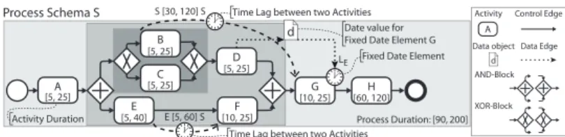
Fig. 1.Core Concepts of a Time-Aware Process Model

are well structured [12], e.g., sequences and branchings are specified in terms of nested single-entry single-exit (SESE) blocks. Fig. 1 depicts an example of a well structured process model with the grey areas indicating respective blocks. Each process model contains a unique start and end node, and may be composed of control flow patterns like sequence, parallel split (ANDsplit), synchronization (ANDjoin), exclusive choice (XORsplit), and simple merge (XORjoin) (cf. Fig. 1).

At run time,process instances may be created and executed according to the defined process model. We assume that a process instance is logically represented by a clone of the respective process model augmented with instance-specific information. If a process model contains XOR-blocks, uncertainty is introduced since not all instances perform exactly the same set of activities. The concept of execution path allows us to identify which activities and control connectors are actually performed during the execution of a particular process instance.

We base our ATAPIS framework on the time patterns (TP) (cf. Sect. 2).

Specifically, we focus on the patterns being most relevant in practice [10]. In detail:

Anactivity duration(TP2) defines the minimum and maximum time span [d_min, d_max] (0≤d_min≤d_max) allowed for executing a particular activity (or node, in general). We assume that each activity has an assigned duration. Since control connectors are automatically executed, we may assume a fixed duration for them (e.g., [0,1]). In turn, aprocess duration[d_min, d_max] represents the time span allowed for executing a process instance.

Time lags between two activities(TP1) restrict the time span allowed between the starting and/or ending instants of two arbitrary activities of a process model [10]. In Fig. 1, a time lag is visualized through a dashed edge between the source and target activity. The label of the edge specifies the constraint according to the following template: hISi[tmin, t_max]hITi(−∞ ≤t_min≤tmax≤ ∞);

hISi,hITi ∈ {S, E}mark the instant (i.e., starting or ending) of the source and target activity the time lag applies to. In turn, [t_min, t_max] represents the range allowed for the time span between instantshI_SiandhI_Ti. Finally, note that a control edge implicitly represents anE[0,∞]Stime lag between the two activities.

Fixed date elements(TP4) allow restricting activity execution in relation to a specific date (e.g., a deadline). Generally, the value of a fixed date element is specific to a process instance. Fig. 1 visualizes a fixed date element through a clock symbol attached to the activity. Thereby, labelhDi ∈ {ES, LS, EE, LE} represents the activity’s earliest start date (ES), latest start date (LS), earliest completion date (E_E), or latest completion date (L_E).

Fig. 1 shows an example of a process model exhibiting temporal constraints.

Note that, although some of the symbols used for visualizing the temporal con-

(5)

straints resemble BPMN timer events, their semantics is quite different and should not be mixed up.

3.2 Temporal Consistency of Time-Aware Processes

A time-aware process model is executed by performing its activities and control connectors, while obeying a set of temporal constraints. We denote a process model as temporally consistent if it is possible to perform all execution paths without violating the temporal constraints involved. Temporal consistency of a time-aware process model (and its instances) constitutes a fundamental prerequisite for its robust and error-free execution [1,4]. For any PAIS supporting time-aware processes, therefore, a crucial task is to check temporal consistency of the process model at design time as well as to monitor and re-check corresponding instances during run time. This is particularly challenging since temporal constraints might interact with each other resulting in complex interdependcies (e.g., a future deadline might restrict the duration of some or all preceding activities).

Whether a time-aware process model is temporally consistent can be checked by mapping it to a conditional simple temporal network (CSTN)—a problem known from artificial intelligence [6]. In ATAPIS, we use CSTN since it allows us to exploit and reusechecking algorithmsfor a well founded model representing temporal constraints. Finally, CSTN allows capturing the complex interdependencies between constraints, which cannot be captured in process models.

Definition 1 (Conditional Simple Temporal Network). A Conditional Simple Temporal Network (CSTN) is a 6-tuple hT,C, L,OT,O, Pi, where:

– T is a set of real-valued variables, called time-points;

– P is a finite set of propositional letters (or propositions);

– L:T →P^∗ is a function assigning a label to each time-point inT; a label is any (possibly empty) conjunction of (positive or negative) letters fromP.¹ – C is a set of labeled simple temporal constraints (constraint in the following);

each constraint cXY ∈ C has the formcXY =h[x, y]XY, βi, whereX, Y ∈ T,

−∞ ≤x≤y≤ ∞, andβ ∈P^∗ is a label.

– OT ⊆ T is a set of observation time-points;

– O:P → OT is a bijection that associates a unique observation time-point to each propositional letter from P.

Time-pointsrepresent instantaneous events that may be, for example, associated with the start / end of activities. In turn, atobservation time-points a decision regarding possible execution paths is made. More formally, when executing observation time-pointP, the truth-value of the associated proposition (i.e., O⁻¹(P)) is determined. Aconstraint cXY =h[x, y]XY, βiexpresses that the time span between time-pointsX andY must be at leastxand at mosty, i.e.,Y −X∈[x, y].

Thelabel attached to each time-point (constraint) indicates possible executions of the CSTN, i.e., a particular time-point (constraint) will be only considered if

1 In the following we use small Greek lettersα, β, . . .to denote arbitrary labels. The empty label is denoted by .

(6)

AS AE

FS FE

GS GE

DS DE

HS HE

ES EE

BS BE

CS CE

PS PE

Time Model M

Z

ANDsplit G H

A

B

C ANDjoin

XORsplit

p? XORjoin D

‹[5, 25], □^›

‹[5, 40], □^› ‹[10, 25], □^›

‹[0, 1], □^› ^{‹[0, 1],}□^› ‹[10, 25], □^› ‹[60, 120], □^›

‹[0, 1], □^›

‹[5, 25], p›

‹[5, 25], ¬p›

‹[0, 1], □^› ^{‹[5, 25],}□^›

‹[0, 1], p›

‹[0, 1], ¬p›

‹[5, 60], □^›

‹[90, 200], ◊›

‹[0, ∞], □^›

‹[30, 120], p›

‹[0, ∞], p›

‹[0,

∞], ¬p›

E F

Time-Point Observation

Time-Point

Activity Mapping Temporal Constraint

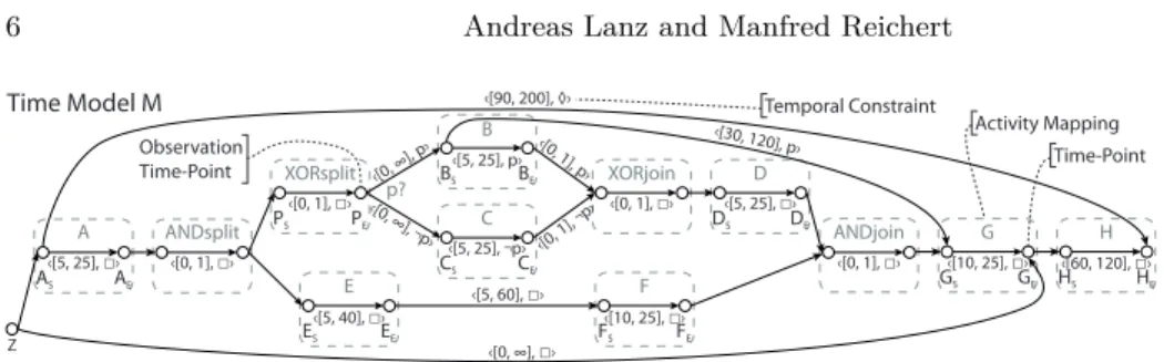
Fig. 2.CSTN Representation of the Process Model from Fig. 1

the corresponding label is satisfiable in the respective instance. Fig. 2 depicts the CSTN corresponding to the process model from Fig. 1.

The solution to a CSTN can be defined as follows [6]:

Definition 2 (Scenario and Solution).Given a CSTNS=hT,C, L,OT,O, Pi, a scenario over setP is a functionsP :P→ {true, f alse} that assigns a truth- value to each proposition in P.

A solution for CSTNS under scenariosP then corresponds to a complete set of assignments to all time-pointsX ∈ T withsP(L(X)) =true, which satisfies all constraints h[x, y]XY, βi ∈ C for whichsP(β) =true holds.

We denote the CSTN corresponding to a time-aware process model as its time model. The required mapping can roughly be described as follows [7]: First, the control flow of the process model is mapped to a CSTN. Particularly, each control flow element implicitly represents a temporal constraint. Each activity, ANDsplit, ANDjoin, and XORjoinni is represented as a pair of time-pointsNiS andNiE, corresponding to the starting / ending instant of the respective node. In turn, for an XORsplit, the ending instant (i.e.,NiE) is represented by an observation time-point. Next, a constrainth[dmin, dmax]N_iSN_iE, iis added betweenNiSand NiE representing the duration [dmin, dmax] of the node. Further, for any control edge between nodesni andnj, a constrainth[0,∞]N_iEN_jS, iis added between the time-points representing the ending instant ofni and starting instant ofnj. If the source of the edge is an XORsplit, in addition, the label of the constraint is augmented by propositionp=O⁻¹(P). The latter represents the decision made at the corresponding observation time-pointP, i.e., the label of the constraint h[0,∞]_N_iE_N_jS, βibelonging to the “true”-branch is set toβpand the one of the

“false”-branch to β¬p.² Further, the labels of all constraints and time-points corresponding to activities, connectors and control edges in the XOR-block are augmented by eitherpor¬pdepending on the branch they belong to.

Next, temporal constraints are mapped to the CSTN. Atime laghI_Si[t_min, t_max]hI_Ticorresponds to a constrainth[t_min, t_max]_N_ih

ISiNjhITi,L(N_ih_IS_i)∧L(NjhITi)i between the two time-points representing the respective instants of nodes n_i andnj. In turn, afixed date element is initially represented as a constrainth[0,

∞]ZN_hDi,L(N_hDi)iwithZbeing a special time-point representing time “0”. During run time, value [0,∞] of the constraint will be updated according to the actual

2 Note that this can be easily extended to consider more than two branches, but for the sake of simplicity, we only consider two branches in this paper.

(7)

fixed date chosen. Finally, process duration [d_min, d_max] is represented as constrainth[d_min, d_max]_N_0S_N_kE, ibetween the time-points representing the starting instantN_0S of the first and the ending instantN_kEof the last node of the process.

As example consider Fig. 2. Note that the labels of the constraints representing the XOR-block are either set topor¬p. For the sake of readability, all edges without annotation are assumed to have boundsh[0,∞], i.

Based on Def. 2, we formally define the notion oftemporal consistency for time-aware process models.

Definition 3 (Temporal Consistency).A CSTNhT,C, L,OT,O, Piis called weakly consistent iff for each scenariosP at least one solution exists [15].

A time-aware process model is denoted as temporally consistent iff the corre- sponding time model (i.e., its CSTN representation) is weakly consistent.

When executing a time-aware process model, temporal consistency of the respective instances needs to be continuously monitored and re-checked. For this purpose, theminimal network of a CSTN must be determined.

Definition 4 (Minimal Network). The minimal network of a CSTN S = hT,C, L,OT,O, Pi is the unique CSTN M = hT,C⁰, L,OT,O, Pi having the same set of solutions as S and each value allowed by any constraintc∈ C⁰ being part of at least one solution ofS.

For any CSTNS a minimal network exists iffS isweakly consistent. In particular, such a minimal network provides a restricted set of constraints: As long as the value of each time-point is consistent with all constraints referring to it, we can guarantee that the entire CSTN is weakly consistent. Besidesexplicit constraints c ∈ C we obtain when mapping the process model to the CSTN, the minimal network containsimplicit constraints between any pair of time-points that may occur in the same execution path. Note that these implicit constraints represent the effects the explicit constraints have on the overall CSTN (i.e., they represent interdependencies between explicit constraints). The implicit constraints are derived from the explicit ones when determining the minimal network. How to determine the minimal network is described in [15].

When executing a process instance, the minimal network of the time model created at design time is cloned. Thisinstance time model is then kept up-to-date with the actual temporal state of the process instance (e.g., deadline, activity start and completion times). Further, it is used to monitor and re-check temporal consistency of the instance [7]. Cloning the time model becomes necessary as the temporal state of each process instance is unique; i.e., no two instances have exactly the same instance time model.

4 Change Operations for Time-aware Processes

Standard change patterns adapting process instances without temporal constraints have been extensively studied in literature [12]. This section discusses how respective change operations may be transferred to time-aware processes. Sect. 4.1

(8)

Operation Informal Description Control Flow Changes

InsertSerial(n₁, n₂, n_new, [d_min, d_max])

Inserts node n_new with duration [d_min, d_max] between directly succeeding nodesn₁andn₂.

InsertP ar(n1, n2, nnew, [dmin, dmax])

Inserts nodennew with duration [dmin, dmax] in parallel to the SESE block defined byn1andn2.

InsertCond(n₁, n₂, n_new, [d_min, d_max], c)

Inserts noden_newwith duration [d_min, d_max] and conditioncas well as an XOR block between succeeding nodesn₁andn₂. DeleteActivity(n) Deletes activityn.^†

Temporal Constraints Changes InsertT imeLag(n1, n2, typetl,

[t_min, t_max])

Inserts a time lag [tmin, tmax] between nodesn1andn2. Thereby, type_tl ∈ {start-start, start-end, end-start, end-end} describes whether the time lag is inserted between the start of the two activities, the start ofn₁and the end ofn₂, the end ofn₁and the start ofn₂, or the end of the two activities.

InsertF DE(n, type_{f de}) Adds a fixed date element of type type_{f de} ∈ {ES, LS, EE, LE} to noden.

DeleteT imeLag(n1, n2, typetl) Deletes the time lag of typetypetlbetween nodesn1andn2.^† DeleteF DE(n, typef de) Deletes a fixed date element of typetypef defrom noden.^†

†Delete operations are not considered in this paper, but are discussed in a technical report [8].

Table 2.Basic Change Operations

presents the change operations applicable to time-aware processes. Sect. 4.2 then provides an in-depth discussion of these operations and shows how they can be extended to ensure temporal consistency of a changed process instance.

4.1 Basic Change Operations

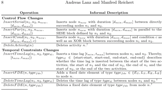
When changing a process instance or—more generally—its process model, soundness must be ensured. To achieve this, ATAPIS abstracts from low-levelchange primitives(e.g., adding an edge or node) to higher-levelchange operationswith well-defined pre- and post-conditions (e.g., inserting a node serially between two succeeding nodes) [12]. Applied to a sound process model, such a high-level change operation guarantees that the modified process model is structurally and behaviourally sound as well [12]. The upper part of Tab. 2 shows selected change operations required for structurally modifying a process instance. Note that respective operations may be combined to realize more complex change patterns [12] (e.g., move activity). ATAPIS extends the set of structural change operations by change operations that allow modifying the temporal constraints of a process model, e.g., inserting a time lag (see the bottom of Tab. 2). Altogether, the operations allow changing a time-aware process instance, while guaranteeing soundness of the corresponding process model. Due to lack of space, this paper restricts itself to insert operations. A detailed presentation of delete operations is provided in a technical report [8].

4.2 Applying Change Operations to Time-aware Processes

When modifying the model of a time-aware process instance, it must be ensured that the resulting process instance is temporally consistent. This section defines basic criteria ensuring that the application of a change operation does not result in a temporally inconsistent process instance. We further analyze the local impact

(9)

<[max{cmin,dmin}, cmax], β>

<[dmin,dmax], β>

<[0, cmax-dmin], β> <[0, cmax-dmin], β>

AS<..., β>AE XS XE BS<..., β>BE

<[cmin, cmax], β>

<..., β> <..., β>

AS AE BS BE

d_min ≤ t_max

A X

[dmin,dmax] B A

[dminX,dmax]

B

E [tmin, tmax] S E [tmin, tmax] S

A

[dminX,dmax]

B

InsertSerial(A, B, X, [dmin,dmax])

E [tmin, tmax] S Process Model

Time Model

Fig. 3.Change OperationInsert Serial

InsertSerial(n1,n2,nnew,[dmin,dmax])*

Pre succ(n1 ) =n2 ,∀h[cmin, cmax]N1E N2S, βi ∈ C:cmax≥dmin Init γ=L(N1E)∧L(N2S)

Post// Update process model:

. . .

// Add mapping to instance time model:

AddT imeP oint(NnewS , γ),AddT imeP oint(NnewE , γ), AddConstraint(NnewS , NnewE ,[dmin, dmax], γ),

AddConstraint(N1E , NnewS ,[0,∞], γ),AddConstraint(NnewE , N2S ,[0,∞], γ), // Adapt instance time model:

∀h[cmin, cmax]N1E N2S, βi ∈ C:U pdateConstraint(N1E , NnewS ,[0, cmax−dmin], β), U pdateConstraint(NnewE , N2S ,[0, cmax−dmin], β),

U pdateConstraint(N1E , N2S ,[max{cmin, dmin}, cmax)], β)

*The complete version of the algorithm is provided in [8].

Algorithm 1: InsertSerial

a particular change operation has on the temporal properties of the respective process model, i.e., its temporal constraints.

When applying a change operation to a process instance, state-specific pre- and post-conditions must be met [12]. Although these are not explicitly considered in this paper, they apply to time-aware processes as well. Furthermore, any time-related, instance-specific data (e.g., activity start and completion times) is maintained in the correspondinginstance time model (cf. Sect. 3.2), i.e., it is sufficient to only consider the current instance time model of the process instance.

Inserting an Activity Serially.InsertSerial(n1, n2, nnew,[dmin, dmax]) is the first change operation we consider. It allows inserting nodennew with duration [dmin, dmax] between directly succeeding nodesn1 andn2(cf. Fig. 3). Regarding the temporal properties of the resulting process model, the insertion of nnew

might first and foremost increase the minimum time distance betweenn1 and n₂ tod_min. By contrast, the maximum distance between the two nodes is not affected by the change as the newly added control connectors do not constrain it.

Accordingly, if for the instance time model the minimum durationd_min is compli- ant with any implicit or explicit constrainth[c_min, c_max]_N_1E_N_2S, βibetween the ending instant of n₁and the starting instant of n₂(i.e.,d_min≤c_max), the node insertion will not affect temporal consistency of the process instance.³ Remember that each value of each constraint in the instance time model is part of at least one solution (cf. Def. 4), i.e., one viable execution of the process model. After adding the node to the process instance, the mapping of this node and the control edges must be added to the instance time model as well. Further, the instance time model must be locally adapted to properly reflect the changes. In particular, the constraint between the ending instant of n1and the starting instant of n2must be updated to [max{cmin, dmin}, cmax] in order to consider the new minimum

3 Note that any implicit constrainth[cmin, cmax]N_1EN_2S, βiis always at least as restrictive as any explicit time lagE[tmin, tmax]S betweenn1 andn2.

(10)

<[max{cmin,dmin}, tmax], β c>

<[cmin, cmax], β ¬c>

<[dmin,dmax], β c>

<[0, cmax-dmin], β c> <[0, cmax-dmin], β c>

AS AE

XS XE

BS BE

GsSGsE GjSGjE

<[cmin, cmax], β>

AS AE BS BE

dmin ≤ tmax

A

[dminX,dmax]

B

E [tmin, tmax] S

c¬c

Gs Gj

A

[dminX,dmax]

B

InsertCond(A, B, X, [dmin,dmax])

Time Model

Fig. 4.Change OperationInsert Conditional

InsertCond(n1,n2,nnew,[dmin,dmax],c)*

Pre succ(n1 ) =n2 ,∀h[cmin, cmax]N1E N2S, βi ∈ C:cmax≥dmin Init γ=L(N1E)∧L(N2S)

Post// Update process model:

. . .

// Add mapping to instance time model:

AddT imeP oint(GsS , γ),AddObservationT imeP oint(GsE , c, γ), AddConstraint(GsS , GsE ,[0,1], γ),

AddT imeP oint(NnewS , γ),AddT imeP oint(NnewE , γc), AddConstraint(NnewS , NnewE ,[dmin, dmax], γc), . . .

AddConstraint(GsE , GjS ,[0,∞], γ¬c), // Adapt instance time model:

. . .

∀h[cmin, cmax]N1E N2S, βi ∈ C:U pdateConstraint(N1E , N2S ,[cmin, cmax], β¬c), AddConstraint(N1E , N2S ,[max{cmin, dmin}, cmax], βc)

*The complete version of the algorithm is provided in [8].

Algorithm 2:InsertCond

distance between the two nodes (cf. Fig. 3), i.e., certain values permitted by the old constraint might no longer be part of any solution. It further becomes evident that the constraints corresponding to the two newly added control edges must be initialized to [0, c_max−d_min] (cf. Fig. 3). Algorithm 1 defines the pre- and post-conditions for applying change operation InsertSerial to a process instance.

The changes applied to the instance time model need to be propagated to all other constraints in order to remove values no longer contributing to any solution.

Note that this must be accomplished before performing any other change or resuming the execution of the process instance. Practically, this means that the minimality of the changed instance time model needs to be restored. This may be achieved by applying the same algorithm as the one initially used for determining the minimal time model (cf. Sect. 3.2).

Inserting an Activity in Parallel. From a temporal point of view, change operationInsertPar (cf. Tab. 2) is similar toInsertSerial. Node nnew (together with ANDsplit and ANDjoin nodes) is inserted “serially” between nodesn1 and n2—the temporal effects of the enclosed SESE block are already considered in the implicit constraint betweenn1 andn2. A detailed discussion is provided in [8].

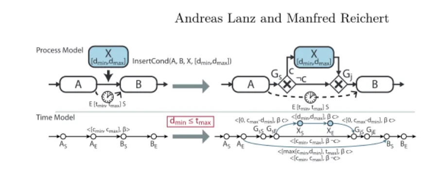
Inserting an Activity Conditionally.Change operationInsertCond(n1, n2, n_new,[d_min, d_max], c) inserts noden_new conditionally between succeeding nodes n₁ andn₂. This change is accomplished by first inserting XORsplitg_sand XOR- join g_j sequentially between n₁ andn₂ and then n_new conditionally between g_s andg_j (cf. Fig. 4). The transition conditions of the control edges linkingg_s and its successors are set toc and¬c, respectively. When adding XORsplitg_s and condition c/¬c to the process model, a set of additional execution paths results; i.e., each execution path of the old process model, which containsn1and n2, can now be mapped to two execution paths: one withc =f alse(i.e.,¬c)

(11)

<[max(cmin,tmin), min(cmax,tmax)], β>

AS AE BS BE

<[cmin, cmax], β>

AS AE BS BE

t_min ≤ c_max tmax ≥ cmin

A B

E [tmin, tmax] S InsertTimeLag(A, B, start-start,

[tmin,tmax])

A B

Time Model

Fig. 5.Change OperationInsert Time Lag

InsertTimeLag(n1,n2,typetl,[tmin,tmax]) Pre hISi=_S _typetl_{= start-*}

E typetl= end-* ,hITi=_S _typetl_{= *-start}

E typetl= *-end (L(N1hISi)∧L(N2hITi)) is satisfiable

∀h[cmin, cmax]N1hISiN2hITi, βi ∈ C:cmin≤tmax∧tmin≤cmax Post// Update process model:

AddT imeLag(n1, n2,hISi[tmin, tmax]hITi) // Add mapping to instance time model:

AddConstraint(N1hISi, N2hITi,[tmin, tmax], L(N1E)∧L(N2S)) // Adapt instance time model:

∀h[cmin, cmax]N1E N2S, βi ∈ C:

U pdateConstraint(N1hISi, N2hITi,[max{cmin, tmin},min{cmax, tmax}], β)

Algorithm 3: InsertTimeLag

representing the previous execution path and one with c =true representing the new path containing n_new between n₁ and n₂. Hence, for any execution path containingn_new,InsertCond has similar effects asInsertSerial. In turn, any execution path not containing n_newremains unchanged (except for the added XORsplit and XORjoin, that constitute silent nodes). Altogether, forInsertCond similar pre-conditions as forInsertSerial hold (cf. Algorithm 1).

In the context of a process instance change, the corresponding instance time model needs to be adapted by adding the mappings of the inserted elements as shown in Fig. 4. Note that this results in a new observation time-pointGsE

and proposition c to the instance time model (cf. Sect. 3.2). Accordingly, the labels of the temporal constraints representingnnew and the two control edges connecting it with g_s andg_j must be set to βc withβ being the label of the original constraint between N_1E andN_2S. In turn, the label of the constraint corresponding to the control edge between g_s and g_j must be set to β¬c. Fi- nally, the constraint between the ending instant ofn₁ and the starting one ofn₂ needs to be updated: The label of the original constraint must be augmented by proposition¬cresulting in constrainth[c_min, c_max]_N_1E_N_2S, β¬ci. Further, another constrainth[max{cmin, dmin}, cmax]N_1EN_2S, βcicontaining propositioncmust be added between the two time-points. The latter corresponds to the casennew is executed between the two nodes. Algorithm 2 defines the pre- and post-conditions ofInsertCond. When applying this operation, again the minimality of the adapted instance time model must be restored. This is required before performing any other change or resuming the execution of the process instance.

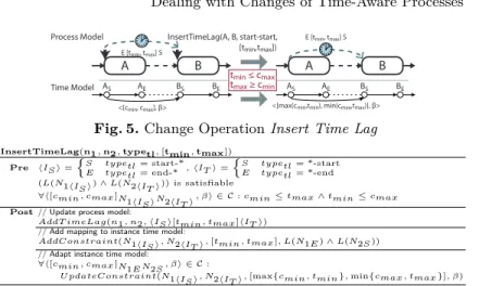
Inserting a Time Lag. Operation InsertTimeLag(n₁, n₂, type_tl,[t_min, t_max]) allows adding a time lag between activitiesn₁ andn₂. The instants the time lag refers to are specified by parametertype_tl. Adding a time lag is only possible if there exists at least one execution path containing both nodes [9]. The instance time model is then adapted by adding a constrainth[tmin, tmax]N_1h_IS_iN_2h_IT_i, βibe- tween the time-points representing the respective instants (start vs. end) of the two nodes. Basically, this updates each implicit constrainth[cmin, cmax]N_1h_IS_iN_2h_IT_i, βi. Note that this is only possible if the resulting constraint [max{cmin, tmin},

(12)

min{c_max, t_max}] in the adapted instance time model still permits at least one value, i.e., it allows for at least one possible solution. Accordingly, in order to apply the operation it must holdc_min≤t_max∧t_min ≤c_max. Algorithm 3 defines the pre- and post-conditions. After updating the temporal constraints, minimality of the adapted instance time model must be restored.

Inserting a Fixed Date Element.Inserting a fixed date element (i.e., opera- tionInsertFDE) is equivalent to adding a time lag between the special time-point Z (indicating time “0”) and the respective instant of the node (cf. Sect. 3.2) [8].

5 Analyzing the Effects of Change Operations

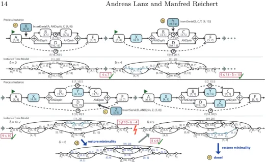
When changing a time-aware process instance both the process model and the instance time model must be updated. In this context, the minimality of the instance time model must be restored after each change operation. Only then it can be ensured that another change within the same change transaction may be applied without violating temporal consistency of the process instance. However, calculating the minimal network of a CSTN is expensive regarding computation time, i.e., its complexity isO(n³2^k) withnbeing the number of time-points andk the number of observation time-points in the CSTN. Consequently, there might be significant delays when applying multiple change operations to large time-aware process instances. This becomes even more pressing in the context of process schema evolution [12] when migrating a potentially large set of process instances to a new schema version (i.e., process model). Hence, the maximum effect a particular change has on the instance time model must be estimated. Based on this estimation, it becomes possible to decide whether another change operation may be applied without need to restore minimality of the instance time model first.

When applying the change operations from Sect. 4.2 to the respective instance time model, two types of changes result: adding a temporal constraint or making an existing one more restrictive. Hence, it is sufficient to consider the effects a basic change has on a minimal time model. Regarding changes that make an existing constraint more restrictive, Theorem 1 shows how their maximum effects can be estimated.

Theorem 1 (Restricting a constraint in a minimal network). LetM = hT,CM, L,OT,O, Pi be a minimal CSTN and M^∗ = hT,CM^∗, L, OT,O, Pi the CSTN derived from M by replacing constraint cAB = h[x, y]AB, βi ∈ CM

with the more restrictive constraint c^∗_AB =h[x+σ, y−ρ]AB, βi;σ, ρ≥0; i.e., C_M^∗ =CM\cAB∪ {c^∗_AB}.

Then: For the minimal network N =hT,CN, L,OT,O, Pi of M^∗ it holds:

for any constraint c⁰_XY =h[x⁰, y⁰]XY, γi ∈ CN the lower bound is increased by at most δ= max{σ, ρ} and the upper bound is decreased by at mostδ compared to the original constraint c_XY =h[x, y]XY, γi ∈ CM. Formally:

∀h[x, y]_XY, γi ∈ C_M,h[x⁰, y⁰]_XY, γi ∈ C_N : (x≤x⁰≤x+δ)∧(y≥y⁰≥y−δ) A proof of Theorem 1 can be found in [8]. Assume that due to a change a constraint [x, y]_XY in the time model is restricted to [x^∗, y^∗]_XY = [x+ρ, y−σ]_XY

(13)

and afterwards minimality of the time model is restored. Theorem 1 now states that any constraint [u, v]_{U V} in the original time model is restricted to at most [u⁰, v⁰]_{U V} = [u+δ, v−δ]_{U V} withδ= max{ρ, σ}in the new time model.

Reconsider operationInsertSerial. Assume that the instance time model is adapted as described by Algorithm 1. The next step would be to restore minimality of this instance time model. First of all, note that the constraints introduced by the newly added activity and control edges do not affect the other constraints when restoring minimality. By construction, their effects are already incorporated in the constraint between time-points N1E andN2S, which is updated in the context of the operation (cf. Algorithm 1; see [2] for details). The only change having an effect on the resulting instance time model is the one restricting constraint [cmin, cmax] betweenN1E andN2S to [max{cmin, dmin}, cmax]. Note that if the constraint is not changed (i.e.,dmin ≤cmin), the existing constraints of the instance time model also need not be changed. Otherwise, the lower bound of the constraint is increased byδ=dmin−cmin. Theorem 1 implies that the upper and lower bound of any other constraint in the new instance time model will be restricted by at mostδ as well. Thus we are able to approximate the maximum difference between the new instance time model and the original one.

From this we can conclude that when applying another insert operation, it will be sufficient to verify that any precondition referring to a constrainth[x, y]XY, βi of the instance time model is satisfied for the respective approximated constraint h[x+δ, y−δ]_XY, βias well. In this case, the insert operation may be applied without violating the temporal consistency of the process instance. In particular, and this is a fundamental advantage of ATAPIS, we need not restore minimality of the modified instance time model prior to the application of the operation. By contrast, if the precondition is not met for the approximated constraint, it might still be possible to apply the change without violating temporal consistency. In this case, however, minimality of the modified instance time model must be first restored before deciding whether the change may be applied.

Similar rules apply to all other insert operations. RegardingInsertCond (cf.

Algorithm 2), in particular, the change relevant to the instance time model is the one restricting the constraint between time-points N1E and N2S to [max{cmin, dmin}, cmax], i.e., the impact on the other constraints is at most δ = max{0, dmin−cmin}. Finally, for InsertTimeLag, the maximum impact corresponds toδ= max{0, tmin−cmin, tmax−cmax} (cf. Algorithm 3).

Based on these observations it becomes possible to apply a sequence of change operations to a process instance within the same transaction without need to restore minimality of the instance time model after each change. If a sequence of change operations op₁, . . . , op_n with impacts δ₁, . . . , δ_n shall be applied to a process instance, it will be sufficient to consider the aggregated impact of the previously applied operations. Practically speaking, for operation op_i, approximated constraint [x+Pi−1

j=1δj, y−Pi−1

j=1δj]XY needs to be considered to determine whether the operation may be applied. Note that this will significantly reduce complexity when applying multiple change operations. However, the actual savings depend on the strictness of the constraints of the time-aware process