Dynamic Allocation and Pricing: A Mechanism Design Approach

Dynamic Allocation and Pricing: A Mechanism Design Approach

Benny Moldovanu

September 2011

Modern Revenue Management

Starts with US Airline Deregulation Act of 1978.

Today mainstream business practice (airlines, trains, hotels, car rentals, holiday resorts, advertising, intelligent metering devices, etc..) Considerable gap between practitioners and academics in the …eld Major academic textbook : The Theory and Practice of Revenue Management by K. T. Talluri and G.J. van Ryzin

Basic RM Questions (Talluri & van Ryzin)

Quantity decisions: How to allocate capacity/output to di¤erent segments, products or channels ? When to withhold products from the market ?

Structural decisions: Which selling format ? (posted prices, negotiations, auctions, etc..). Which features for particular format

?(segmentation, volume discounts, bundling, etc..)

Pricing decisions: How to set posted prices, reserve prices ? How to price di¤erentiate ? How to price over time ? How to markdown over life time ?

Towards a Modern Theory of RM

Necessary blend of

1 The elegant dynamic modelsfrom the OR, MS, CS , Econ (search) literatures with historical focus on "grand, centralized

optimization" and/or "ad-hoc", intuitive mechanisms.

2 The rich, classical mechanism design literature with historical focus oninformation/incentives in staticsettings.

Blend fruitful for numerous applications.

Reviewed Papers (joint work with A. Gershkov)

Dynamic Revenue Maximization with Heterogeneous Objects: A Mechanism Design Approach,AEJ: Microeconomics 2009

E¢ cient Sequential Assignment with Incomplete Information,GEB 2010

Revenue Maximization for the Dynamic Knapsack Problem, TE 2011 (also joint with D. Dizdar)

Learning About The Future and Dynamic E¢ ciency, AER 2009 Optimal Search, Learning, and Implementation,mimeo 2010.

E¢ cient Dynamic Allocation with Strategic Arrivals, mimeo 2011

The Gallego & van Ryzin Model (MS 94 ) I

Revenue Maximizing (RM) seller has n identical objects that perish after deadlineT.

Agents arrive according to a Poisson process with intensity λ.

Agents’values are private information, represented by I.I.D random variables X_i =X on[0,+∞)with common c.d.f. F.

Agents desire one object only, and can only be served upon arrival (no recall)

After an item is assigned, it cannot be reallocated.

The Poisson Process

The Poisson process with intensity λis a continuous-time counting process f^N(t),t 0g^{such that:}

1 N(0) =0

2 Independent increments: the numbers of events in disjoint time intervals are random variables independent from each other.

3 Stationary increments: the probability distribution of the number of events in any time interval only depends on the length of the interval.

4 N(t+τ) N(t), the number of events in time interval (t,t+τ] follows a Poisson distribution with parameterλτ :

P[N(t+τ) N(t) =k] = ^e

λτ(λτ)^k

k! , k =0,1,2...

5 The probability distribution of the waiting time until the next event is an exponential distribution.

Gallego & van Ryzin II

Gallego & van Ryzin restrict attention to posted prices: at each point in timet, seller sets pricep_t that needs to be paid by any buyer that arrives att.

Main Results:

1 Optimal posted-price revenue is concave in the number of objects, and in time until deadline.

2 Time pattern of optimal prices: Downward trend, interrupted by upward jumps after each sale.

3 Fixed price is approximately optimal if min (n,λT)is large enough.

New Research Questions

General Mechanisms

Multiple, Heterogenous Objects Multi-Unit Demand

Learning about Demand Recall and Strategic Arrivals

Derman-Liebermann-Ross (MS 72)

each item i =1, ..,m is characterized by a "quality"q_i with 0 qm qm 1 ... q1

n agents arrive sequentially, one agent per period agents can only be served upon arrival

after an item is assigned, it cannot be reallocated each agent is characterized by a "type"x_j

if an item with typeqi 0 is assigned to an agent with type xj, this agent enjoys a utility of q_ix_j

agents’types are IID random variablesXi =X on [0,+_∞)with common cdf. F

DLR Model II

Theorem (DLR 72)

Consider the arrival of an agent with type x_k in period k 1. There exist k+1constants0=ak,k a1,k ... a0,k =_∞ such that:

The dynamically e¢ cient policy assigns the item with quality q_(i) if x_k 2 (a_i,k,a_{i 1,k}]

The constants are given recursively by a_i,k+1 =

Z _{ai 1,k}

a_i,k

xdF(x) +a_i,kF(a_i,k) +a_{i 1,k}[1 F(a_{i 1,k})]

where we set +_∞ 0= _∞ 0=0.

In a problem with n periods total expected welfare is given by Wn =_∑ⁿ_i=1q_(i)ai,n+1.

Majorization: De…nition

De…nition

For any n tupleγ= (γ₁,γ₂, ..,γ_n) letγ_(j) denote thejthlargest

coordinate (so that γ_(n) γ_{(n 1)} ... γ₍₁₎). Vector α= (α1,α2, ..,αn) is majorized byβ = (β₁,β₂, ..,β_n)and we writeα βif the following system of n 1 inequalities and one equality is satis…ed:

α(1) β₍₁₎ α₍₁₎+α₍₂₎ β₍₁₎+β₍₂₎

... ...

α₍₁₎+α₍₂₎+..α_{(n 1)} β₍₁₎+β₍₂₎+β_{(n 1)} α₍₁₎+α₍₂₎+..+α_(n) = β₍₁₎+β₍₂₎+..+β_(n)

We say that αisweakly sub-majorized byβ and we writeα w βif all relations above hold with weak inequality.

Majorization: Main Results (Marshall & Olkin, 79)

Theorem

1 α β if and only if there exists a doubly stochastic matrix Q such that α= βQ.

2 A function Ψ:Rⁿ !R is called Schur-convex ifΨ(α) _Ψ(β)for any α,β such that α β.

3 Let Ψ:Rⁿ !R be symmetric with continuous partial derivatives.

Then Ψ is Schur-convex if and only if for all(y1, ...,yn)2^{Rn and all} i,j 2 f^{1, ..,n}git holds that

∂Ψ(y₁, ...,y_n)

∂y_i

∂Ψ(y₁, ...,y_n)

∂y_j (y_i y_j) 0.

Majorization in the DLR Model

Let X_(i),k denote thei th highest order statistic out ofk copies of X,and let µ_(i),k denote its expectation.

Let S_n denote the set of permutations off^{1,2, ..,n}g^{.For each} permutation σ2 ^{Sn,de…ne µσ}n = µ_(σ(1)),n , µ_(σ(2)),n , ..., µ_(σ(n)),n Total expected welfare in a static problem where n agents arrive simultaneously is given by ∑ⁿi=1q_(i)µ_(i),n.

Theorem

The n tuple f^ai,n+1gⁿi=1 is majorized by the n tuplef^µi,ngⁿi=1 . In particular, there exist n permutations f^σigⁿi=1 and non-negative weights f^wigⁿi=1 such that ∑i=1w_i =1 and

∑ⁿi=1w_iµ^σ

i

n = (a_1,n+1,a_2,n+1, ..,a_n,n+1).

Albright’s Model (MS 74 ) I

Welfare Maximizing (WM) seller hasm items.

Each itemi =1, ..,n is characterized by a "quality"q_i with 0 qn qn 1 ... q1

If an item with qualityqi 0 is assigned to an agent with typexj this agent has utility q_ix_j

Complete information: current type is known upon arrival; future types are IID random variablesX_i =X on [0,+∞) with common c.d.f. F.

Poisson arrivals, unit demand, deadline, etc..as in Gallego & van Ryzin.

The Welfare Maximizing (WM) Allocation

Theorem (Albright)

Denote by Πt the set of items available at t, with cardinality k_t.There exist n+1 unique functions

∞ y₀(t) y₁(t) ..y_n(t) 0, 8^t

which do not depend on the q’s such that if an agent with type x arrives at time t, it is optimal to assign him the j’th highest element of Πt if x 2[y_j(t), y_{j 1}(t)) and not to assign any object if x <y_kt(t).

1 For each k,the function y_k(t)satis…es y_k⁰(t) = λRy_{k 1}

y_k (1 F(x))dx.

2 The expected welfare from timet on is given byW_t =_∑^k_i=^t₁q_(i)y_i(t), whereq_(i) is the i’th highest element ofΠt.

Albright: lllustration.

Example

There are three objects; λ=1; the distribution of agents’types is F(x) =1 e ^x.The following …gure depicts the solution forT =5:

0 1 2 3 4 5

0.0 0.5 1.0 1.5 2.0

t y

Second Order Stochastic Dominance I

Theorem

Consider two distributions of agents’types F and G such that

µ_F =µ_G =µand such that F second-order stochastically dominates G (in particular F has a lower variance than G).Then it holds that:

1 For any time t,and for any n,the vector f^yi^F(t)gⁿi=1 of optimal cuto¤s under F is weakly sub-majorized by the vector f^yi^G(t)gⁿi=1 of optimal cuto¤s under G.

2 For any time t and for any set of available objects at t, Πt 6=∅, the expected welfare in the e¢ cient dynamic allocation under F is lower than that under G.

SSD: Illustration

Example

Let F(x) =x on[0,1]so that F is IFR and thusF SSD

G(x) =1 e ^2x.There is one object;λ=1;T =5.y₁^F(t) =1 ₇²_t is the dashed line, y₁^G(t) = ¹₂ln[6 t]is the solid line.

0 1 2 3 4 5 6

0.0 0.2 0.4 0.6 0.8 1.0 1.2

t y

Second Order Stochastic Dominance (Static Counterpart)

Theorem (De La Cal & Caracamo, J. Appl. Prob. 06)

Consider two distributions of agents’types F and G . The following two assertions are equivalent:

1 F second-order stochastically dominates G .

2 For any n,the n tuple f^µF_(i),ngⁿi=1 of mean order statistics under F is majorized by the n tuple f^µG_(i),ngⁿi=1of mean order statistics under G. Corollary

Consider two distributions of agents’types F and G such that

F second-order stochastically dominates G . Then, for any set of available objects, expected welfare in the e¢ cient static allocation under F is lower than that under G .

The Loss from Sequentiality I

Assume that at timet there aren objects left.

Consider scenario where the allocation to all subsequently arriving agents can be made at the deadline T.

Expected welfare at t is given by ∑ⁿi=1q_(i)zi(t),wherezi(t)

represents the expected type of an agent who arrives aftert, and who get assigned to the object with the i th highest quality.

Let Pr_l(t) =e ^{λ(T t)λl(T}_l! ^t)l be the probability that there will be l arrivals,l 1,after timet. Then

z_i(t) =

∑

Pr_l(t)µ_{(l i+1),l} =e ^{λ(T t)}

∑

λ^l(T t)^lµ_{(l i+1),l} l! , 8^i. where let µ_(i),l is the expectation of thei th highest order statistic out of l copies ofX.

The Loss from Sequentiality II

Intuitively,∑ⁿi=1q_(i)[yi(t) zi(t)]measures the welfare loss due to the sequentiality constraint.

Theorem

1 For any period t,and for any n,the vector f^yi(t)gⁿi=1 of optimal cuto¤s in the dynamically e¢ cient allocation of n objects is weakly sub-majorized by the vectorf^zi(t)gⁿi=1.

2 Moreover, lim_n!∞∑ⁿi=1y_i(t) =lim_n!∞∑ⁿi=1z_i(t) =λ(T t)µ, where µis the mean of the distribution of agents’types.

In…nite Horizon & Discounting

In…nite horizon (T =_∞), discount rate r(t) =e ^αt.

Arrival process is a renewal with general inter-arrival distributionB Theorem (Albright MS 1974)

The dynamically e¢ cient cuto¤ curves are stationary (i.e., independent of time) y_n y_{n 1}... y₁.These constants do not depend on the q’s, and are given by the implicit recursion:

(y_k +y_{k 1}+..y₁) = L^B(α) 1 L^B(α)

Z _∞

yk

(1 F(x))dx , 1 k n where L^B is the Laplace-transform of the inter-arrival distribution.

Recall that for random variableX with densityf,theLaplace Transform is given by L(s) =E[e ^sX]

Inter-Arrival Distributions I

De…nition

Let β,γ be two non-negative random variables governed by distributions B,C,respectively. Then B dominates C in theLaplace transform order if

E[e ^sβ] E[e ^sγ] for alls >0 Theorem

Consider two inter-arrival distributions B and C such that B _Lt C .

1 For any …xed distribution of agents’characteristics F,and for any n, the n tuple f^yi^Bgⁿi=1 of optimal cuto¤s under B is weakly

sub-majorized by the n tuple vectorf^yi^Cgⁿi=1 of optimal cuto¤s under C.

2 In particular, for any t,and for anyΠt 6=_∅,the expected welfare from t on in the e¢ cient dynamic allocation under B is lower than

Inter-Arrival Distributions II

De…nition

A non-negative random variableW is called NBU (NWU) if, for every y >0,W is stochastically larger (smaller) than the conditional random variable (W y/W y).

Example

Assume that there is one object, and consider a situation with an NBU (NWU) distribution of abilities with mean µ, and another NBU (NWU) distribution of inter-arrival times with mean ω.Then, the expected welfare under the e¢ cient dynamic policy is lower (higher) than

µLambertW( ¹ ωα)

where the increasing functionLambertW(x) is implicitly de…ned by:

LambertW(x)e^LambertW(x) =x

Mechanisms and Incomplete Info. I

Assume types are private information. If an item with quality q_i 0 is assigned to an agent with type x_j for pricep_i, this agent has utility qixj pi.

W.l.o.g. restrict attention to deterministic, Markovian and direct mechanisms where every agent, upon arrival, reports his characteristic x_i and where, at any point in time t, the mechanism speci…es:

1 a non-random allocation rule (which object is allocated, if any) that only depends ont,on the declared type of the arriving agent, and on the inventory of items available at t.

2 a payment to be made by the arriving agent which depends on t,on the declared type of the agent, and on the inventory of items available att.

Mechanisms II

Theorem

1) An non-randomized, Markovian policyf^Qt(x,Πt)g^t is implementable i¤ at each t it partitions the set of agents’types into k_t +1disjoint intervals such that all types in a given interval obtain the same quality, and such that higher types obtain a higher quality.

2) The associated payment scheme is given by P_t(x,Πt) =

kt

∑

(q_(i:Πt) q_(i+1:Πt))y_i,Πt (t) if x 2[y_j,Πt (t),y_{j 1,Πt}(t)) and by zero otherwise.

Mechanisms III

Corollary

The WM policy is implementable. Payments are the dynamic analogue of the Vickrey-Clarke-Groves mechanism (see also Bergemann and Valimäki, EC 10)

Payments have intuitive interpretation: look at static case with k_t objects andkt +1 agents where, in addition to agent with typex, there are kt "dummies" with typesy_1,Πt (t), y_2,Πt(t), ...,y_kt,Πt (t). Payment for object with the j-highest quality,

∑^ki=^tj(q_(i:Πt) q_(i+1:Πt))y_i,Πt (t)represents the externality imposed by agent with type x on dummies

RM with Heterogenous Objects

Theorem

Assume that the virtual value x ¹_f^F_(x⁽₎^x) is increasing. Then the RM allocation is given by n cut-o¤ functions that do not depend on the available qualities. These functions satisfy:

y_i(t) ^{1 F} (y_i(t)) f (yi(t)) +λ

Z _T

t

[1 F (y_{i 1}(s))]²

f (yi 1(s)) ^ds =λ Z _T

t

[1 F(y_i(s))]² f (yi(s)) ^ds or, equivalently

y_i(t) ^{1 F} (y_i(t))

f (y_i(t)) +R(1_{i 1},t) =R(1_i,t)

where R(1j,t)is the expected revenue at time t from the optimal policy if j identical objects with q =1 are still available at that time.

Proof (Sketch) I

One object with qualityq is available at timet ;agent arriving att gets object ifx_i y₁(t),and no object otherwise. Expected revenue given by

q Z _T

t

y₁(s)h₁(s)ds

whereh₁(s)is the density of waiting time till the …rst arrival of an agent with a value abovey1(s).

By theColoring Theorem,this density equals the density of the …rst arrival in a non-homogenous Poisson process with rate

λ(1 F(y₁(s)),given by

h1(s) =λ(1 F(y1(s))e ^{λRts[1 F(y(z))]dz} for t s T Perform calculus of variation exercise with respect to y₁(t) Use backward induction.

Clearance Sales

Percentage Markdown: Di¤erence between prices of the same product att =0 and t =T, divided by the price att =0.

Pashigian and Bowen (QJE 91) empirically …nd that :

"More expensive apparel items within each product line are frequently sold at a higher average percentage markdown"

Theorem

Assume an RM seller and consider the scenario where at time t =0there are n1>0 items of quality q and n2 >0items of quality s <q,while at time t =T there are l₁ >0 items of quality q , and l₂ >0items of quality s left unsold. Then the percentage markdown is always higher for the higher quality.

Optimal Inventory Design

Theorem

Let y =f^yi(t)gⁿi=1 denote the allocation underlying the RM policy with n objects, and assume that the cost of producing qualities (q₁,q₂, ..q_n)is given by C(q1,q2, ..qn) =_∑ⁿ_i=1φ(qi)whereφ:R !R is strictly increasing, convex and satis…es φ(0) =0. Then

1) The optimal number of objects n is characterized by φ⁰(0)2(y_n +1(0) ^{1 F}(y_n +1(0))

f (y_{n +1}(0)) ^{, yn} (0) ^{1 F} (y_n (0)) f (y_n (0)) ] 2) The optimal qualities q_i are given by:

φ⁰(q_i) =y_i(0) ^{1 F} (y_i(0))

f (yi(0)) ^{, i} =1, ...,n

Multi-Unit Demand: Dynamic Knapsack

An RM seller has capacity C 2R+ that perishes afterT periods.

In each period, impatient agent arrives with quantity request w, and per-unit value v.Type (w,v)is private information to the arriving agent.

Type (w,v)’s utility is given bywv p if at pricep he is allocated a capacityw⁰ w and by p if he is assigned an insu¢ cient capacity w⁰ <w.

Demands are I.I.D across periods, governed by c.d.f. F(w,v)with density f(w,v)>0 on [0,∞)². For allw, the conditional virtual valuev ¹_f^F_(v^(vjw)

j^w) is an unbounded, strictly monotone function ofv.

Complete information optimization model due to Kleywegt &

Papastavrou,OR 01; they do not consider payments.

Dynamic Knapsack: Implementable Policies

A deterministic, Markovian allocation rule for timet with remaining capacityc has the form α^c_t :[0,+_∞)² ! f^1,0g^{where 1} (0)means that the reported capacity demand w is satis…ed (not satis…ed).

Theorem

A policy f^αctg^t,c is implementable i¤ for every t and every c it satis…es:

1) 8(w,v),v⁰ v, α^c_t(w,v) =1 )^αct(w,v⁰) =1.

2) The function wp_t^c(w)is non-decreasing in w,where p^c_t(w) =inff^{v / αc}t(w,v) =1g^.

The maximal, individually rational payment function that implements f^αctg^t,c is given by

q^c_t(w,v) =

(wp^c_t(w) if α^c_t(w,v) =1 0 if α^c_t(w,v) =0

IIlustration: Implementable Policies

Example

Assume T =1. Weightw is realized according to an exponential distribution with parameter λ. Per-unit value is sampled from the following distribution

F(vj^w) = ^{1 e}

λv if w >w

1 e ^λv if w w

where λ>λand w 2(0,c). For observable weight requests, seller charges _λ¹ (¹

λ)per unit if the w ( )w .This implies that wp_t^c(w) =

( _w

λ if w >w

w

λ if w w .

and therefore, wp_t^c(w) is not monotone.

Dynamic Knapsack: RM I

Theorem Assume that:

1 For any w,the hazard rate ₁^f(_F^v₍^j_v^w)

j^w) is non-decreasing in v.

2 For any w⁰ w , and for any v, ₁^f(_F^v₍^j_v^w)

j^w)

f(vj^w0) 1 F(vj^w0).

For each c,t,w let p^c_t(w)denote the recursive solution to the system w p^c_t(w) ^{1 F}(p^c_t(w)j^w)

f(p_t^c(w)j^w) =R (c,T t) R (c w,T t). where R denotes the optimal revenue with R (c,0) = 0 for all c.

Then the underlying allocation whereα^c_t(w,v) =1i¤ if v p_t^c(w)is implementable. In particular, the above system determines the RM policy.

Dynamic Knapsack: RM II

Optimal revenue may not be concave in capacity (see Kleywegt &

Papastavrou,OR 01 for non-concavity in WM) - this is connected to implementation problems.

Under a concavity conditions on the distribution of types, revenue is concave and above system also determines RM policy.

RM policy requires price adjustments for everyc,t,w - complicated dynamics. We construct a static nonlinear price schedule (it uses correlations betweenw andv !) that is asymptotically optimal if min(C,T)is large enough.

Learning about Values: Illustration 1

one object

two agents arrive sequentially, one per period each agent can only be served upon arrival after an item is assigned, it cannot be reallocated valuations x_i are private

valuations distributed independently and uniformly on [0,2]

Illustration 1: continued

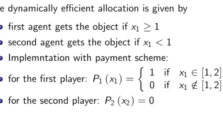
The dynamically e¢ cient allocation is given by

…rst agent gets the object if x₁ 1 second agent gets the object if x₁<1 Implemntation with payment scheme:

for the …rst player: P1(x1) = ^{1 if x1} 2[1,2] 0 if x1 2/[1,2] for the second player: P₂(x₂) =0

Learning about Values: Illustration 2

one object

two agents arrive sequentially, one per period each agent can only be served upon arrival

the designer does not know the distribution of values

with probability 0.5 the distribution of both agents’types is uniform on[0,1]

with probability 0.5 the distribution is uniform[1,2]

Value of keeping vs. value of allocating object

0 1 2

0 1 2

x

Illustration 2: continued

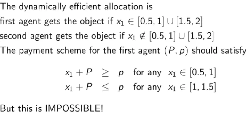
The dynamically e¢ cient allocation is

…rst agent gets the object if x₁ 2[0.5,1][[1.5,2] second agent gets the object if x12/[0.5,1][[1.5,2]

The payment scheme for the …rst agent (P,p)should satisfy:

x₁+P p for any x₁2 [0.5,1] x₁+P p for any x₁2 [1,1.5] But this is IMPOSSIBLE!

Complete Information & Learning

Theorem (Albright, 1977)

Consider the arrival of an agent with type x in period k 1,and denote by χ_k the vector of past reported signals. There exist k+1 functions

0= a_0,k(χ_k,x)) a_1,k(χ_k,x) a_2,k(χ_k,x) ... a_k,kχ_k,x_k) =∞ such that the dynamically e¢ cient policy assigns the item with the i ’th smallest type if x 2 (a_{i 1,k}(χ_k,x),a_i,kχ_k,x)].

Each a_i,k+1(χ_k+1,x_k+1)equals the expected value of the agent’s type to which the item with i th smallest type is assigned in a problem with k periods before the period k signal is observed. These functions do not depend on the q’s.

Incomplete Information & Learning-I

Question: When do cuto¤s exist which

1 are independent of the signal of the current agent and

2 replicate the e¢ cient allocation ? The key element is the set

A_i,k(χ_k) =f^{x :ai 1,k}(χ_k,x)) x<a_i,k(χ_k,x))g^.

B 4 - Incomplete Information & Learning-II

Theorem (Necessary and su¢ cient condition)

The e¢ cient allocation is implementable if and only if for any period k, any object qi and any history Hk the set Ai,k(χ_k)is convex.

Theorem (Su¢ cient condition)

Assume that for any k, χ_k, i 2 f^{0, ..,k}g, the cuto¤ a_i,k(χ_k,x_k)is a Lipschitz function of x_k with constant 1. Then, the e¢ cient dynamic policy is implementable.

Insight taken from the theory of mechanism design with interdependent values (Jehiel & Moldovanu,EC 01)

Su¢ cient Conditions I

Theorem

Assume that for any k,and for any pair of ordered lists of reportsχ_k χ⁰_k that di¤er only in one coordinate, the following conditions hold:

1 Fe_k(xj^χk)%^{FOSD Fek}(xj^χk⁰)

2 E(xj^χk) E(xj^χ0k) _k^∆₁where∆ is size of the di¤erence between χ_k andχ⁰_k

Then, the e¢ cient dynamic policy is implementable.

Su¢ cient Conditions II

Theorem

Assume that the conditional distribution function Fek(xj^{xn, ,xk+1})and density ef_k(xj^{xn, ...,xk+1}) are continuously di¤erentiable with respect to x_k+i for all x and for all n k i 1. If

0 ∂

∂x_k+iFe_k(xj^χk) ¹

n kfe_k(xj^χk) for all x and all n k i 1 then the e¢ cient dynamic policy is implementable.

Illustration

Example

Considerex N(µ,1)with unknown meanµ, and prior beliefs e

µ N(µ₀,¹

τ)with τ>0.

After observing xn, ..xk+1, posterior isµe N(µ,_τ+¹_{n k})with µ= ^τµ_τ+(⁰⁺_{n k}^∑x₎ⁱ , and

Fe_k(xj^{xn, ...,xk+1}) = N(µ,1+ ¹ τ+n k); Fe_k(x+ ^z

τ+ (n k)j^{xn, ..,xi}+z, ..,x_k+1) = F^e_k(xj^{xn, ..,xi, ..,xk+1}) SD holds, and

∂Fe_k(xj^{xn, ..,xk+1})

∂xk+i

= ¹

τ+n kfe_k(xj^{xn, ..,xk+1}) 1 fe(xj^{x , ..,x} )

Remarks

Remark

1 The right-hand side condition says that the function e

F_k x+ _{n k}^z j^{xk+1, .,xk+i} +z,x_k+i+1, .,x_n is non-decreasing in z. In other words, after having made n k observations, a small shift to the right - which moves the value of the distribution upwards - is enough to compensate the downward e¤ect on the distribution’s value caused by an (n k)times larger upward shift in one of the past observations (recall that, by stochastic dominance, higher

observations move the entire distribution downwards).

2 The condition guarantees that8^{i,k,n,∂ai,k}∂x^(χk^k,xk)

1

n k although

∂ai,k(χk,xk)

∂xk 1 seems su¢ cient for the implementation of the e¢ cient allocation. Nevertheless, the long-term e¤ect of each non-terminal observation makes it impossible to obtain tighter conditions that apply generally.

Search for the Lowest Price (Rothschild1973):

Consumer obtains a sequence of prices, and must decide when to stop the (costly) search for a lower price.

Beliefs about distribution of prices updated (in a Bayesian way) after each observation.

Without learning, optimal stopping rule is characterized by a reservation price R : stops search at any price less than equal to R, and continue search at any price higher than R.

If all customers follow such a rule=) well-behaved demand function where sales are a non-increasing function of price

When does the optimal stopping rule with learning have the

reservation price property ? I.e.,when does a priceR(s)exist for each state s such that prices above are rejected, and prices below are accepted ?

Answers to Rothschild’s Question

Stochastic Dominance u^:

Rosen…eld and Shapiro (1981): For all x,k,χ_k and alln k i 1 Z _∞

x

∂

∂x_k+i

Fek(yj^χk)dy 1

n k(1 Fek(xj^χk) Seierstad (1992) : For all x,k andχ_k

n k

∑

i=1

∂

∂xk+i

e

F_k(xj^χk) fe_k(xj^χk)

Us (multiple objects !): For all x ,χ_k ,and alln k i 1

∂

∂x_k+i

Fek(xj^χk) ¹

n kfek(xj^χk)

Non-Bayesian Learning I

Before stage n the designer’s prior belief about the distribution of the …rst type x_n is given by G. Conditional on observingx_n,x_{n 1}...,x_k+1 at stages n,n 1, ...k+1,the belief about the distribution of the next typex =x_k is given by:

Fe_k(xj^{xn, ...,xk+1}) = (1 βⁿ_k)G(x) +βⁿ_k 1

n k

∑

1_[xi,∞)(x), k =1,2, ...n 1 where 0 <βⁿ_k <1 and where1_[z,∞)(x) denotes the indicator function of the set [z,∞).

Theorem

Under "empirical" learning , the e¢ cient dynamic policy can always be implemented under incomplete information.

Non-Bayesian Learning II

Prior to any observation, the designer estimates the unknown distribution to be uniform. Suppose that mobservations were made, and order them in increasing order n

x₍₁₎, ...,x_(m)o

, and let x₍₀₎=0 and x_(m+1)=1. The belief about the distribution of the next type x is given by:

f_k(xj^{xn, ...,xn m+1}) =

m+1 i

∑

1_{[x(i 1),x(i))}(x) (m+1) x_(i) x_{(i 1)}

.

Theorem

Under "maximum entropy" learning, the e¢ cient dynamic policy can always be implemented under incomplete information.

Characterization of Second-Best Mechanism

Theorem

1 At each period k, expected welfare (calculated before the arrival of the period k agent) is a Schur-convex, linear function of the available qualities at that period.

2 The incentive compatible, optimal mechanism (second best) is

deterministic. That is, for every history at period k, H_k, and for every type xk of the agent that arrives at that period, there exists a quality q that is allocated to that agent with probability1 .

3 At each period, the optimal mechanism partitions the type set of the arriving agent into a collection of disjoint intervals such that all types in a given interval obtain the same quality with probability 1, and such that higher types obtain a higher quality.

Outline of Proof

Schur-convexity of expected welfare in a deterministic, incentive compatible mechanisms follows by induction.

) At each periodk it is optimal to leave for the future the "most disperse" set (in the sense of majorization) of feasible qualities that is consistent with incentive compatibility.

) ^Periodk’s optimal allocation must be the "most concentrated"

one that is consistent with monotonicity.

) ^Periodk’s allocation should be either deterministic, or should randomize among at most two neighboring qualities.

Finally, randomization among two neighboring qualities cannot be optimal. This is related to an argument due to Riley & Zeckhauser who studied revenue maximization for 1 seller-1 buyer problem without monotone virtual values.

Patient Agents & Complete Info. (Bertsekas 05)

Seller has 1 object.

Time is discrete, deadlineT.

One new buyer arrives at each period t (arrivals observed by seller).

Buyers have IID values for the object represented by random variable e

v

Buyers are long lived; common discount factor δ.

Patient Agents: Main Result

Theorem

The dynamically e¢ cient policy awards the good in period t if and only if the set of present buyers contains a buyer whose value exceeds a cuto¤ xt. If the good is allocated in period t , it is awarded to the agent with the highest value. The cuto¤s x_t satisfy:

1 xT =0

2 x_t =δE[max(_ev,x_t)],for t <T.In particular the optimal cuto¤ is constant in periods t <T.

Intuition: At the optimum in period t <T, the seller should be indi¤erent between awarding the good to a buyer with value xt, and waiting one more period and getting another draw. Note thatx_t, t >T,also equals the optimal cuto¤ in the in…nite horizon problem with impatient agents !

Patient Agents: Incomplete Information (Board &

Skrzypacz 10)

Assume now that values are private information.

Optimal allocation can be implemented through a series of second-price auctions.

Although optimal cuto¤ is constant for all t <T,reserve prices that implement these cuto¤s decrease over time !

The reserve price makes the cuto¤-type indi¤erent between buying today and tomorrow; Prices thus decline both because discounting and because the risk of losing to a new bidder that comes tomorrow.

Agents with value below cuto¤ but above reserve price refrain from buying: they wait for the "…re-sale" at the last period.

Strategic and Unobservable Arrivals

Designer endowed with indivisible object;

Stream of randomly arriving, long-lived (or patient) agents; arrivals described by a counting processfN(t),t 0gin continuous time Agent’s private information is two-dimensional: arrival time t 0 and value v 0 for the object. Arrival time and value are independent of each other.

Values are I.I.D. random variables with common c.d.f. F,continuos density f.

If an agent arrives att, gets the object at τ t and pays p at τ⁰ 2[t,τ], then her utility is given bye ^δτv e ^δτ0p where δ 2(0,1)is the discount factor.

Designer’s utility is given bye ^δτv (WM) ore ^δτ0p (RM).

Renewals under Complete Information

Theorem (Zuckerman)

A non-negative random variable W is called NBU (new better than old) if, for every y >0,W is stochastically larger than the conditional random variable (W y/W y).

Assume that the arrival process is a renewal, and that the inter-arrival distribution G satis…es the NBU property. Let φdenote the Laplace Transform of G . Then, the optimal policy allocates the object to the …rst arrival whose value is above v where v is the unique solution to

v = ^φ(δ) 1 φ(δ)

Z _∞

v (v v )dF(v)dv.

In particular, recall is never used by the optimal policy, and all allocations occur upon arrival.

Application to RM (Gallien 06)

Private information is characterized by (v_i,t_i,d_i) wherev_i is the value,ti is the arrival time, and di ti is the exit time. The designer’s goal is to maximize revenue.

Assume that arrivals are governed by a renewal process with a NBU distribution, and that the virtual valuation function x ¹_f(^F_x⁽₎^x) is strictly increasing, and denote byH the implied distribution of virtual values. Then, for any d_i, d_i t_i,i =1,2, ..,the revenue maximizing policy is to charge a constant price P whereP is the unique solution to

p= ^φ(δ) 1 φ(δ)

Z _∞

p

(z p)dH(z)dz

The solution coincides with the one found by Gallien for the case di =_∞ (perfect recall) and by GM for the case d_i =t_i (no recall).

Learning from Arrivals: Example

Distribution of values isU[0,1].

Inter-arrival time is known: 1) U[1,2] or 2) U[2,3]. The optimal cuto¤s for a WM designer are

x_[i,j](δ) = ¹ φ_[i,j](δ) ¹

q

1 (φ_[i,j](δ))² where

φ_[i,j](δ) = ^e

iδ e ^jδ

δ .

is the respective Laplace transform.

Fix any δ and note thatx_[1,2] =x_[1,2](δ)>x_[2,3](δ) =x_[2,3]. No recall used

Unknown Arrival Process / Complete Information

Designer does not know the distribution of inter-arrival times:

believes that it is eitherU[1,2]or U[2,3], with equal probabilities.

Under complete information optimal policy is:

1 For T 2(1,2]the cuto¤ is x_[1,2]

2 For T 2(2,3]the cuto¤ is x_[2,3] if there were no arrivals before time 2, otherwise the cuto¤ isx_[1,2]

3 For T >3, the cuto¤ isx_[1,2] if the …rst arrival happened during time interval (1,2], whereas the cuto¤ is x_[2,3] if the …rst arrival happened during (2,3].

Unknown Arrival Process / Incomplete Information

The allocative externality payment, which needs to be paid for the object by an agent arriving att t₁ is

P(t1) = ^{x[1,2] ift1} 2[1,2] x_[2,3] ift1 2(2,3] ^.

Consider type (t,v)with t 2(1,2)andv 2(x_[2,3],x_[1,2]). Truthful reporting yields zero utility since object not allocated to him. But, a report (t⁰,v)wheret⁰ =t+12(2,3)yields utility

e ^δt0 v x_[2,3] >0 .

Truthful reporting under standard Clarke-Groves-Vickrey mechanism is not optimal, and WM dynamic allocation cannot be implemented ! Problem: Informational externality on designer induced by early arrivals.

Subsidizing Early Arrivals I

Subsidy to be paid to agent that arrives at t, independently of whether he gets the object:

S(t) = ^{x[1,2] x[2,3]} >0 if t 2[1,2]

0 if t 2 .

General intuition: LetU(t,t⁰,v)be the utility of an agent with type (t,v)who arrives at t⁰ and optimally reportsv⁰ (given(t⁰,t,v)) in the version of the model where arrivals are observable and where the designer uses the dynamically e¢ cient mechanism.

Choose subsidy scheme S(t⁰)such that the function

U(t,t⁰,v) +e ^δt0S(t⁰)decreases in reported arrival time t⁰ for anyt andv.

Subsidizing Early Arrivals II

Theorem

Assume that there exists M 0such that for any t t⁰ t⁰⁰ in [0,T] and for any v it holds that

U t,t⁰⁰,v U(t,t⁰,v) M(t⁰⁰ t⁰)

Then the subsidy S(t⁰) =e^δt0M(T t⁰)together expected allocative externality payment implements the e¢ cient policy for any history which stops before T.

Let L(t⁰) =sup_{v,t t}0∂U(t,t⁰,v)

∂t⁰ and assume that there exists c(t⁰) L(t⁰)such thatC =R_∞

0 c(z)dz< ∞.The subsidy function S(t⁰) =e^t0δ C

Z _t⁰

0

L(z)dz works for T =∞.

Winner-Pay Mechanisms I

De…nition

A mechanism is calledwinner-pay mechanism if the transfers to all agents that do not get the object are zero.

Theorem

Assume that arrivals are unobservable, and that the arrival process is a known renewal with inter-arrival distribution G . Then a subsidy is not needed for e¢ cient implementation.

Proof.

(Sketch): Show that U(t,t⁰,v)decreases in t⁰ for anyv and for any t t⁰.At allocation, elapsed time from last arrival must be the same, independently of reported arrival time. Price charged depends on elapsed time since last arrival, and on second highest value reported so far. Later arrival postpones allocation ! more arrivals!increases second highest

Winner-Pay Mechanisms II

Theorem

Assume that arrivals are governed by a non-homogenous Poisson/pure-birth process with arrival rate λi(t) whereλ is

non-decreasing in both elapsed time t and the number of arrivals i up to t.

Suppose that there exists a non-decreasing function β(t) such thatλi(t) β(t)for all i,t,and such that R_∞

0 β(t)e ^δtdt < _∞.Then:

1 An optimal stopping rule exists for the setting with observable arrivals.

2 Charging for the object a payment equal to the optimal cuto¤ under observable arrivals, implements the e¢ cient allocation also if arrivals are non-observable. In other words, a subsidy is not needed for e¢ cient implementation.

Calculated Example

Example

Assume that the distribution of values is F(v) =1 e ^v , and consider a non-homogenous Poisson process with rate λ(t) =δ(t+2)ln(t+2) 1.

λis positive and increasing in t,and Z _∞

0 [δ(t+2)ln(t+2) 1]e ^δtdt <∞

Optimal cuto¤y(t) in the optimal stopping problem where arriving agents are short lived is given by:

y⁰ δy = [δ(t+2)ln(t+2) 1]e ^y

The solutiony(t) =ln(t+2) increases int and satis…es all optimality conditions for δ _{2 ln 2}¹ =0.72.Charging P(t) =ln(t+2)implements the e¢ cient dynamic allocation also in the problem with recall and

1