Here, we compare natu- ral carbon uptake in the Southern Ocean simulated with con- temporary eddy parameterizations

(1)

Heiner Dietze^1,2, Julia Getzlaff¹, and Ulrike Löptien^1,2

1GEOMAR Helmholtz Centre for Ocean Research Kiel, Kiel, Germany

2Institute of Geosciences, University of Kiel, Kiel, Germany Correspondence to:Heiner Dietze (heiner.dietze@ifg.uni-kiel.de) Received: 26 October 2016 – Discussion started: 3 November 2016

Revised: 1 March 2017 – Accepted: 3 March 2017 – Published: 27 March 2017

Abstract. The Southern Ocean is a major sink for anthropogenic carbon. Yet, there is no quantitative consensus about how this sink will change when surface winds increase (as they are anticipated to do). Among the tools employed to quantify carbon uptake are global coupled ocean-circulation–

biogeochemical models. Because of computational limita- tions these models still fail to resolve potentially important spatial scales. Instead, processes on these scales are parameterized. There is concern that deficiencies in these so-called eddy parameterizationsmight imprint incorrect sensitivities of projected oceanic carbon uptake. Here, we compare natural carbon uptake in the Southern Ocean simulated with contemporary eddy parameterizations. We find that very differing parameterizations yield surprisingly similar oceanic carbon in response to strengthening winds. In contrast, we find (in an additional simulation) that the carbon uptake does differ substantially when the supply of bioavailable iron is altered within its envelope of uncertainty. We conclude that a more comprehensive understanding of bioavailable iron dynamics will substantially reduce the uncertainty of model- based projections of oceanic carbon uptake.

1 Introduction

More than two decades after the discovery of major glacial and interglacial cycles in the CO₂ concentration of the atmosphere, it is believed that no single mechanism can account for the full amplitude of past CO₂variability (e.g., Sig- man and Boyle, 2000). There is, however, growing evidence

that the variability in the extent, to which deep-water masses are isolated from the atmosphere in the Southern Ocean, is among the major drivers regulating atmospheric CO₂ variability. In this context, the role of wind-driven upwelling is of special interest (e.g., Lenton and Matear, 2007; Lovenduski et al., 2007; Marshall and Speer, 2012), especially since An- derson et al. (2009) linked increased ventilation of deep water to the deglacial rise in atmospheric CO2.

There is also evidence that wind-driven upwelling will shape the future evolution of atmospheric CO2 concentrations: observations during the recent decades show a strong upward trend of the dominant atmospheric mode of climate variability in the Southern Hemisphere (Marshall, 2003), which is, most likely, anthropogenically driven (e.g., Polvani et al., 2011). This upward trend of the so-calledSouthern An- nular Modeis related to stronger surface winds and a poleward shift of the westerlies and is projected by climate scenarios to intensify (e.g., Simpkins and Karpechko, 2012). As to how the projected wind changes will quantitatively link to upwelling of deep carbon-rich waters (which in turn affects atmospheric CO2concentrations) is, however, not com- prehensively understood. The current generation of coupled ocean-circulation–biogeochemical models still struggles to retrace observed trends (Lenton et al., 2013) and the models differ considerably with regards to their representation of anthropogenic carbon in the Southern Ocean (Frölicher et al., 2015).

For now we know that the Southern Ocean (here defined as the region south of 40^◦S) accounts for more than 40 % of the total annual oceanic CO₂uptake (Takahashi et al., 2009).

(2)

Further, there is evidence, based on inversions of atmospheric CO₂ concentrations (Le Quérér et al., 2007) and trends in the difference between partial pressures of CO₂ in the surface ocean and the atmosphere (Metzl, 2009; Takahashi et al., 2009), that the uptake of CO₂ in the Southern Ocean has been declining up to the mid-2000s (Landschützer et al., 2015; Xue et al., 2015).

The link between variability in surface winds and South- ern Ocean carbon uptake remains, however, inconclusive:

global ocean-carbon models driven by observed wind patterns suggest that increased winds drive an increased expo- sure of carbon-rich deepwater to the surface. This leads to an overall reduced gradient between the atmosphere and the surface ocean and, subsequently, to a decreased oceanic CO2up- take. More specifically, all state-of-the-art coarse-resolution ocean models suggest that the enhanced equatorward Ekman transport associated with a poleward shift and intensification of the Southern Hemisphere westerlies results in an increased circulation in the subpolar meridional overturning cell (e.g., Saenko et al., 2005; Hall and Visbeck, 2002; Getzlaff et al., 2016). This implies an increased upwelling of deep water, rich in dissolved inorganic carbon, south of the circumpolar flow (e.g., Zickfeldet al., 2007; Lenton and Matear, 2007;

Lovenduski et al., 2008; Verdy al., 2007).

On the other hand, high-resolution models that explicitly resolve eddies rather than parameterizing their effect show that stronger westerlies induce an increased eddy activity and suggest that the associated eddy fluxes could compen- sate initial increases in northward Ekman transport (Hallberg and Gnanadesikan, 2006; Hogg et al., 2008; Screen et al., 2009; Thompson and Solomon, 2002). As a consequence, the upwelling, associated air–sea carbon fluxes, isopycnal tilt and the transport of the Antarctic Circumpolar Current (ACC) should be rather insensitive towards changes in the wind forcing. In line with the high-resolution models, observations by Argo floats do not reveal any changes in isopycnal tilt as a response to increasing winds (Böning et al., 2008).

This suggests that the wind-induced upwelling can indeed be compensated by eddy fluxes.

To date, earth system models that are used to project air–

sea carbon fluxes do not explicitly resolve eddy fluxes. Be- cause of computational constraints the relevant spacial scales cannot be resolved and the respective processes have to be parameterized. Typically, non-eddy-resolving ocean models employ the parameterization of Gent and McWilliams (1990) (hereafter GM) to account for the effects of (unresolved) tur- bulent lateral advection. The “strength” of these effects in the GM parameterization is determined by a parameter, the so- calledthickness diffusivity. In the past, for pragmatic reasons, the thickness diffusivity has been set to a globally constant value. On physical grounds, however, there is no justifica- tion for a global uniform thickness diffusivity. To the con- trary, satellite observations and eddy-resolving modeling, for example, clearly reveal that eddy activity varies strongly in space and time. This implies that the effect of eddies on the

mean flow is inhomogeneously distributed over the ocean.

Thus, recent advances have been aimed at taking the variability of the eddy field into account by parameterizing the thickness diffusivity as a local function of, for example, strat- ification,Eady growth rate, or a combination of the Eady growth rate, theRossby radiusand theRhines scale. The results of these advances towards a more realistic closure for the thickness diffusivity clearly show that mean (resolved) properties such as, for example, the simulated strength of the ACC or the meridional overturning circulation (MOC) are sensitive towards the choice of the closure (Eden et al., 2009;

Viebahn, 2010). This suggests that the simulated upwelling of deep carbon-rich waters in the Southern Ocean may as well be sensitive to the choice of the closure.

In the present study, we test differing closures for GM’s thickness diffusivity in a global coarse-resolution coupled ocean-circulation–biogeochemical model (which comprises carbon). The focus is on how the choice of a closure affects the sensitivity of carbon uptake in response to increasing winds in the Southern Ocean. To this end, we will revisit the apparently discrepant responses to trends in the Southern Annular Mode of (1) coarse-resolution models on the one hand, and (2) eddy-resolving models and observations on the other hand.

In order to put our results concerning uncertainties associated with physical processes into perspective, we compare it with the uncertainty that is associated with uncomprehen- sively understood deposition of bioavailable iron.

The following Sect. 2 describes our global coupled ocean- circulation–biogeochemical model configurations and the respective simulations. The Sects. 2.1.1 and 2.2.1 give a short introduction to eddy parameterizations and iron, respectively.

In Sect. 3 we compare all simulations with one another. The focus is on the simulated carbon uptake of the Southern Ocean and related processes. The paper ends with a conclu- sive summary in Sect. 4.

2 Model

This study is based on simulations with the Modular Ocean Model (MOM), version MOM4p1. Specifically we use the ocean-ice component of the CM2Mc configuration coupled to the Biology Light Iron Nutrients and Gasses (BLING) ecosystem model of Galbraith et al. (2010). We force the ocean-circulation model with climatological atmospheric conditions (Normal Year Forcingof Large and Yeager, 2004).

Our configuration is identical to the one used and described in Galbraith et al. (2010).

The nominal zonal resolution is 3^◦. The meridional resolution varies from 3^◦in mid-latitudes to 2–3^◦near the equator.

Additional regions of enhanced meridional resolution are the latitudes of the Drake Passage and respective latitudes on the Northern Hemisphere. In the Arctic, a tripolar grid is applied to avoid discontinuities at the North Pole (see Griffies et al.,

(3)

from the spin-ups are evaluated in Appendix A.

Each of the three spin-ups is extended in order to assess the sensitivity of simulated natural carbon uptake in the South- ern Ocean towards anticipated wind changes. In each of the extensions the magnitude of the wind speeds south of 40^◦S is increased at a rate of 14 % in 50 years. This increase is consistent with results from reanalysis for the period 1958 to 2007 (Lovenduski et al., 2013). In our setups the increase in winds affects predominantly the input of momentum. Note, however, that air–sea heat and gas exchange are also affected via their respective bulk formulas.

In the remainder of this Section we describe our sensitivity experiments in more detail. These experiments explore the impact of differing eddy parameterizations and compare it to uncertainties that are related to biogeochemical responses to changes in air–sea deposition of bioavailable iron. Table 1 summarizes the experimental setup. The following subsec- tions are organized as follows:

– Section 2.1 starts with an overview of approaches to parameterize the effect of eddies in coarse-resolution models (Sect. 2.1.1), followed by an explicit description of our model setups and the respective simulations with differing eddy parameterizations in Sect. 2.1.2.

– Section 2.2 starts with an overview of the effects of iron on primary production and associated carbon sequestration (Sect. 2.2.1), followed by an explicit description of our simulation with altered supply of bioavailable iron to the ocean in Sect. 2.2.2.

2.1 Eddy parameterizations 2.1.1 Introduction

The simulation of oceanic motion (driven by pressure gradient force, gravity and viscous friction) by numerically solv- ing theprimitive equationsis intimately coupled to the question of how to proceed with sub-grid processes that cannot be resolved but are known to affect processes on the resolved scales. The reason is that computational costs and constraints

FMCD The model configuration and integration procedure is identical to CON except for the eddy parameterization which is set to the default CM2.1 setting in Galbraith et al. (2010) with a spatially varying thickness diffusivity.

E&G The model configuration and integration procedure is identical to CON except for the eddy parameterization which is set to spatially varying following Eden and Great- batch (2008) in its simplified form of Eden et al. (2009).

IRON The underlying model configuration, the spin-up and the integration procedure is identical to FMCD except for air–sea fluxes of iron south of 40^◦S which are increased by a rate corresponding to a doubling in 50 years.

render it typically impossible to resolve all spatial scales that are involved in the dynamics of interest.

For global ocean-circulation models, that are coupled to biogeochemical (carbon) models, the explicit resolution of mesoscale processes has – so far – been already beyond computational capacities. Hence, to date, model-based projections of oceanic carbon uptake rely on parameterizations of mesoscale processes.

Historically, attempts to parameterize mesoscale processes in ocean models started with relatively simple, horizontal, down-gradientLaplaciandiffusion with associated constant diffusivities on the order of 1000 m²s⁻¹. Early on, it has been realized by Veronis (1975) that the associated horizontal mixing results in too-intense diapycnal mixing in regions of sloped isopycnals (see McDougall and Church, 1985). As a workaround Redi (1982) proposed to transform the horizontal diffusion tensor such that scalars and momentum are mixed only along isopycnals. The conundrum with this so- calledisopycnal mixingscheme, however, is that it (wrongly) implies that eddies do not have any effects on the dynamics in

(4)

regions where the density distribution is governed by either temperature or salinity only.

To date, virtually all climate models apply the parameterization of GM to account for the effects of unresolved ocean eddies. GM constitutes a positive definite sink of the global potential energy by introducing a purely adiabatic extra advection. The parameterization is also referred to asthickness diffusion (even though its inventors now consider the term to be misleading; Gent, 2011) which vividly describes the effect of thickness diffusion on layers bounded by two isopycnals – that is, evening out local differences in layer thickness. Associated with GM is a parameter, often dubbedthick- ness diffusivity, orκ, which prescribes the speed with which differences in isopycnal layer thicknesses are evened out. It is agreed thatκ should be spatially varying in order to account for the fact that eddy activity is not homogeneously distributed over the globe. But as for concerns about how it should or could be calculated in a coarse-resolution model, there is no consensus.

The most pragmatic choice is setting κ constant (see Gent et al., 1995). Other approaches include “. . . an attempt to tune away model bias, rather than an attempt to make a poorly represented process more physical. . . ” (Gnanade- sikan et al., 2005), or calibration with results from eddy- resolving models (Eden and Greatbatch, 2008).

2.1.2 Sensitivity experiments – thickness diffusivities The choice of the thickness diffusivity closure has been shown to cause local effects in the Southern Ocean such as differing ACC transports (Eden et al., 2009), and differing sensitivities of the MOC towards wind stress changes with global implications (Viebahn, 2010). The question of which closure yields the most realistic results has not been unan- imously answered yet. Among the associated problems are the following: (1) there are no direct MOC observations in the Southern Ocean. (2) Different model configurations or closures typically feature differing – albeit likewise-biased – climatologies (e.g., sea ice, Bryan et al., 2014) which renders the ranking of model sensitivities inconclusive. As regards simulated MOC changes in response to changing winds, there is some guidance from intercomparison with eddy- resolving models (see Viebahn, 2010). This guidance, however, is based on the assumption that eddy-resolving models are realistic, albeit they are also biased.

Our aim here is to quantify the uncertainty in the uptake of natural carbon in the Southern Ocean that is associated with the choice of the closure for thickness diffusivity in a global coupled ocean-circulation–biogeochemical model. To this end, we compare results from three contemporary closures for the thickness diffusivity κ dubbed CON, FMCD and E&G:

– CON: closure is constant in space and time: κ= 600 m²s⁻¹.

– FMCD: closure is a function of space (longitude, latitude, tapering to the bottom and the surface) and time as a function of the horizontal density gradient averaged from 100 to 200 m depth:

κ=α|∇_zρ|^z L²g

ρ0N0

. (1)

The dimensionless α=0.07, the length scale L=50 km, and the Brunt–Väisälä frequency N₀=0.004 s⁻¹ are tuning constants; g=9.8 m s⁻¹ is the standard acceleration of free fall andρ₀=1035 is the reference density for the Boussinesq approximation and |∇_zρ|^z is the average of the horizontal density gradient taken over the depth range 100 to 2000 m.

Maximum and minimum values forκ are set to 2000 and 200 m²s⁻¹, respectively.

– E&G: closure is a function of space (longitude, latitude, depth) and time as proposed by Eden and Greatbatch (2008) based on considerations of the eddy kinetic energy budget:

κ=L²σ, (2)

where the inverse timescaleσ= |∂_yb|/N= |f ∂_zu|/N is related to the Coriolis parameterf, the vertical shear of the mean flow∂_zuand the Brunt–Väisälä frequency N;σ is also referred to as the Eady growth rate which is a measure of the baroclinic instability. The length scale L is set as L=min(L_R, L_Rhi), with the local first baroclinic Rossby radiusL_R and the Rhines scale LRhi=√

u/β. The Rhines scale defines the spatial scale at which planetary rotation causes zonal jets. It is a function of the eddy horizontal velocityuandβ (the latitu- dinal gradient off).

In addition to the thickness diffusivities discussed above we apply an isopycnal diffusivity of 600 m²s⁻¹in all configurations presented here.

2.2 Iron deposition 2.2.1 Introduction

Iron, although an abundant element on earth, is present only at very low concentrations in the ocean. Typically, the vertical distribution shows a profile which is similar to nitrate or phosphate (e.g., Johnson et al., 1997), with lower concentrations at the surface (<0.2 nmol kg⁻¹) and concentrations peaking further down in the thermocline (at around 1 nmol kg⁻¹). Another similarity to macro-nutrients is that in vast oceanic regions, the growth of autotrophs is limited by the availability of iron (see Boyd and Ellwood, 2010).

Among the iron-limited regions is the Southern Ocean, where direct observational evidence shows that changes in

(5)

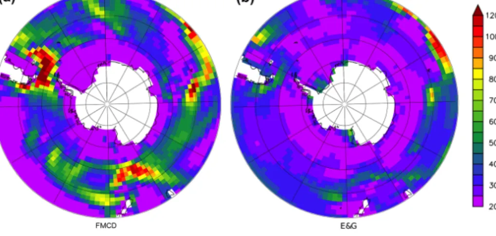
Figure 1.Vertical mean thickness diffusivities (upper 500 m), averaged over the last 20 years of spin-up. Panel(a)refers to configuration FMCD and(b)refers to configuration E&G. The units are meters squared per second (m²s⁻¹).

iron supply affect the biotic uptake of carbon and its export to depth (Smetacek et al., 2012).

To this end a consensus has been reached in the literature.

The global oceanic iron cycle is an important agent in the global biogeochemical carbon cycle. But, even so, there is still a large discrepancy between the evidential importance of iron dynamics and our poor quantitative understanding thereof. One expression of this discrepancy is that, on the one hand, the biogeochemical protocols for the CMIP6 Ocean Model Intercomparison Project (see Eyring et al., 2016) now rank simulated dissolved iron concentration as “priority 1”

model output (Orr et al., 2016, their Table 5) while, on the other hand, the same protocols suggest not to initialize the models with observations of dissolved iron because suitable data compilations are not available yet.

In short, neither sources nor sinks of dissolved iron in the ocean are well constrained and data of standing stocks are so sketchy that the scientific community recommends not to use these data for simulations. Among the reasons for this dire situation are challenges such as the following: (1) sources and sinks overlap spatially such that standing stocks of iron cannot constrain the (speed of the) iron cycling (Frants et al., 2016); (2) aeolian sources of iron are intermittent and thus hard to quantify, (e.g., Duggen et al., 2010; Olgun et al., 2011); (3) physicochemical stabilization is not well understood such that, for example, the importance of iron origi- nating from hydrothermal vents remains uncertain (Resing et al., 2015); and (4) iron sinks such as scavenging and precip- itation are not well understood (e.g., Tagliabue et al., 2014) and an explicit representation of the essential iron-binding ligand dynamics in models has only just begun (Völker and Tagliabue, 2015).

2.2.2 Sensitivity experiment – iron supply

The cycling of iron in the ocean is not well constrained: in terms of an average residence time in the ocean, contempo-

rary models differ by two orders of magnitudes (4 to 600 years; Tagliabue et al., 2016). It is straightforward to assume that the large uncertainty in the supply and cycling of iron affects the sensitivity of simulated oceanic carbon uptake. As a first step towards relating uncertainties in iron dynamics with oceanic carbon uptake, we conduct a sensitivity experiment where we change the aeolian supply of bioavailable iron to the ocean. (Note that fathoming the full range of uncertainty is beyond the scope of this manuscript.) The rationale behind this experiment is as follows: in a warming world the amount of airborne dust is increasing due to vegetation loss, dune remobilization (e.g., Bhattachan et al., 2012) and glacier re- treat (e.g., Bullard, 2013). In line with this reasoning, model- aided estimates by Mahowald et al. (2010) suggest that the increase may well correspond to a doubling over the 20th century over much of the globe. In our experimental design, we follow Krishnamurthy et al. (2009) and assume in our sensitivity experimentIRONthat the deposition of bioavailable iron, associated with aeolian dust, does also double over a period of 50 years. Other than these changes of iron supply, the simulation IRON is identical to the simulation FMCD.

3 Results

Figures 1 and 2 show thickness diffusivities in the configurations FMCD and E&G at the end of their spin-up: we find a≈40 % difference in the average diffusivities between the contemporary concepts FMCD, E&G and the constant value of 600 m²s⁻¹ in CON. The thickness diffusivities in both FMCD and E&G vary substantially in space (Fig. 1) although not in unison: in FMCD we find large thickness diffusivities in the region of the ACC, which is in line with results from high-resolution models and observations (e.g., Frenger et al., 2013; Hallberg and Gnanadesikan, 2006). In E&G the elevated values in the ACC are less pronounced and elevated diffusivities appear in the Weddell and Ross sea.

(6)

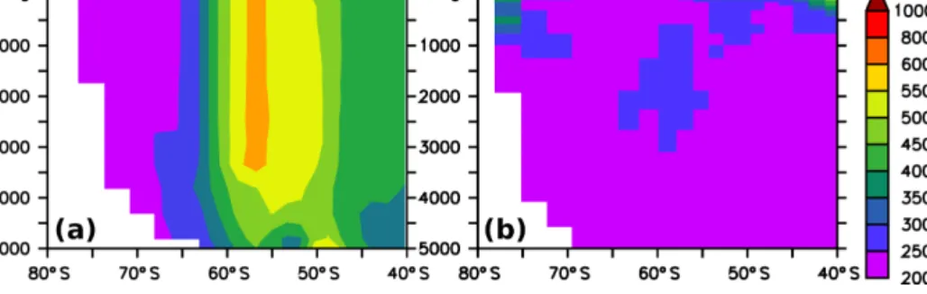
Figure 2.Zonal mean thickness diffusivities, averaged over the last 20 years of spin-up. Panels(a)and(b)refer to configuration FMCD and E&G, respectively. The units are meters squared per second (m²s⁻¹).

In E&G, in contrast to FMCD, even the large values decay rapidly with depth (Fig. 2). Both FMCD and E&G peak lo- cally at values twice as large as the constant thickness diffusion applied in CON (Fig. 1). Even so, the zonal averages of FMCD and E&G are typically lower than in CON (Fig. 2).

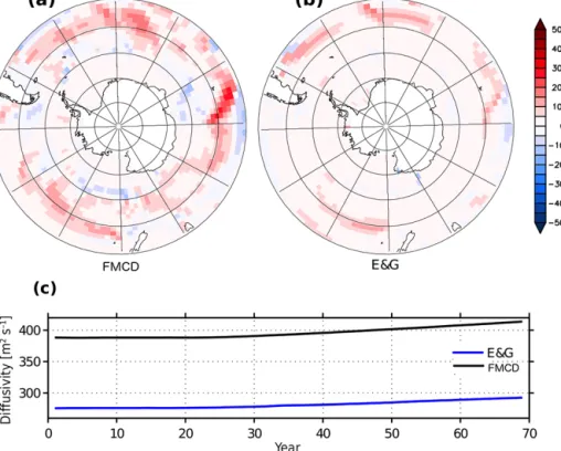
The thickness diffusivities vary not only substantially among the configurations at the end of the respective spin-ups, but they do also feature differing sensitivities towards increasing winds. While the thickness diffusivities in CON stay constant at 600 m²s⁻¹, the thickness diffusivities in both FMCD and E&G show a similar – albeit not identical – pattern of increase (Fig. 3a and b). Expressed in terms of a thickness diffusivity averaged over the whole Southern Ocean, the increase is linearly related to the wind increase and peaks at 16 and 25 m²s⁻¹in the configurations E&G and FMCD, respectively (Fig. 3c).

In the following, we summarize the oceanic responses to the combination of increasing winds and changing thickness diffusivities:

– Ekman pumping. The vertical velocities that are driven by the horizontal divergence of Ekman transports increase along with the winds by up to 50 m yr⁻¹(Fig. 4).

The responses of all considered configurations are al- most identical (i.e. indistinguishable by eye), indicating that surface current/wind effects (see Dietze and Löp- tien, 2016) differ very little among the configurations.

This also indicates that the kinetic energy transferred from the atmosphere to the ocean is very similar in all of the configurations.

– Meridional overturning. In all configurations the increased winds drive an enhanced meridional overturning with similar patterns and amplitudes (Fig. 5). Also common to all configurations is that the fraction of meridional overturning that is effected by the respective GM parameterization is opposing the increasing trend (i.e. the changes in Fig. 6 are negative over most of the region). The magnitude of this counter effect, however, differs considerably among the configurations. Figure 6 reveals that the counter effect, or “eddy compensation”

as it is also referred to, peaks at 2 Sv in CON and E&G

while FMCD features much higher values up to 4 Sv.

Note that these results do not support the hypothesis that a more complex definition of the thickness diffusivity (such as in E&G and FMCD) does necessarily amount to an increase of the (parameterized) eddy compensation relative to the original pragmatic choice (see Gent et al., 1995) of setting it constant (such as in CON).

– Air–sea heat flux. The air–sea heat flux averaged over the Southern Ocean is an indicator of diabatic heat fluxes in its thermocline because the heat exchanged between the surface mixed layer and the atmosphere has to be replaced from somewhere. This view neglects trends in sea surface temperature and near-surface oceanic heat fluxes entering the region. Figure 7a shows the temporal evolution of heat exchanged with the atmosphere.

The most striking feature is that in all configurations the air–sea heat exchange is relatively constant, even though the winds increase considerably. Other than that, there is a small offset between the configurations, indicating differences in the meridional overturning of heat. Short term anomalies in time, such as between year 30 and 40 in FMCD and E&G in Fig. 7a, are correlated with sea-ice extent.

– Sea-ice cover. Among the biggest concerns in prepa- ration of the configurations was sea ice. The reason is that sea ice caps the ocean, shielding it from air–sea exchange of heat and carbon. Thus, sea-ice dynamics are coupled to carbon uptake and a comparison of model configurations that feature differing sea-ice covers can be challenging. The intimate coupling between sea-ice cover and air–sea fluxes is evident in Fig. 7a and b. All anomalies in the heat fluxes (such as, for example, between year 30 and 40 in E&G and FMCD) have their counterpart in sea-ice extent, suggesting that less sea- ice results in more cooling of the ocean as vaster areas of relatively warm ocean waters are exposed to the cold polar atmosphere. Fortunately, the temporal evolution of sea-ice extent is very similar among the configurations.

If it were not (e.g., as in the configurations compared by

(7)

Figure 3.Temporal evolution of thickness diffusivity, averaged over the upper 1000 m. Panels(a)and(b)refer to changes (the average of year 65–69 minus the average over the last 20 years of the spin-up) effected by increasing winds in simulation FMCD and E&G, respectively.

(c)shows the evolution of the domain-averaged (south of 40^◦S) diffusivity simulated with FMCD (black line) and E&G (blue line). The first 20 years correspond to the end of respective spin-ups. From year 20 onward, the winds increase. The units are meters squared per second (m²s⁻¹). Configuration CON (with a constant 600 m²s⁻¹) is not shown.

Table 2.Simulated linear trends in carbon uptake south of 40^◦S in response to increasing (14 % in 50 years) winds. The units are PgC/(1000 yr²). Negative trends indicate declining oceanic uptake.

Simulation Trend in 95 % confidence

tag carbon uptake interval

CON −5.4 −5.5,−5.3

FMCD −4.6 −4.7,−4.5

E&G −4.2 −4.3,−4.1

IRON −2.7 −2.8,−2.6

Bryan et al., 2014), the interpretation of results would not be straightforward.

Despite some significant differences in simulated physics among the configurations FMCD, E&G and CON (such as, for example, differing levels of eddy compensation) the simulated oceanic carbon uptake rates are surprisingly similar, irrespective of the underlying eddy parameterization (Fig. 7c): expressed in terms of linear trends, the uptake rates differ by less than 13 % (calculated as the standard deviation divided by the mean of the three trends; see Table 2).

The deviations from a linear decrease such as, for example, the “anomaly” between year 60 and 70 in configuration

Figure 4.Acceleration of Ekman pumping as simulated with configuration FMCD (and IRON). The unit is meters per year (m yr⁻¹ for 50 years). Regions with increased upwelling (or reduced pumping) are colored in red.

CON are small and correspond to changes in ice extent with less sea ice being associated with stronger outgassing (or less uptake) of carbon.

(8)

Figure 5.Change in meridional overturning (after 49 years of increasing winds) in units Sv (10⁶m³s⁻¹). Positive values indicate increasing overturning in response to increasing winds. Panels(a),(b)and(c)refer to simulations CON, FMCD and E&G, respectively.

Figure 6.Change of that fraction of the meridional overturning that is effected by the respective GM parameterizations (after 49 years of increasing winds) in units Sv (10⁶m³s⁻¹). Negative values indicate a damping of the overturning in response to increasing winds. Panels (a),(b)and(c)refer to simulations CON, FMCD and E&G, respectively.

Figure 7. Oceanic response to increasing winds south of 40^◦S (spatially and annually averaged). Panel (a) shows air–sea heat fluxes with negative values denoting oceanic cooling),(b) shows ice-covered area and(c)shows oceanic carbon uptake with positive values denoting oceanic uptake. The line colors refer to experiments as indicated in the legend. The first 20 years correspond to the end of respective spin-ups. From year 20 onward, the winds increase.

In contrast, changes to the deposition of bioavailable iron within its “envelope of uncertainty” in experiment IRON do effect substantial changes in the carbon uptake rates (43 % reduction relative to the mean of the trends of CON, FMCD and E&G; see Table 2). Figure 7 shows that IRON is the only

simulation in which the Southern Ocean remains a carbon sink throughout the simulated time period.

4 Summary and conclusion

Global coupled ocean-circulation–biogeochemical models predict an increase of oceanic natural CO₂ outgassing due to strengthening winds in the Southern Ocean (e.g., Loven- duski et al., 2013). These predictions contain a considerable degree of uncertainty, some of which is associated with what Lovenduski et al. (2016) refer to as intermodel “structural differences”.

In the present study, we compare two sources of uncertainties in simulated carbon uptake in response to increasing winds in the Southern Ocean with one another: (1) the uncertainty related to actively discussed details in the contemporary GM parameterization, which mimics the effects of unresolved mesoscale circulation on the resolved larger-scale circulation in coarse-resolution models. Specifically, we explore different definitions of the respective thickness diffusivity. (2) To put the results into perspective, we also consider the uncertainty that is related to the rather unconstrained deposition of bioavailable iron to the sun-lit surface ocean.

The investigation of the GM parameterization is motivated by studies such as of Farnetti and Gent (2011) and Gent and Danabasoglu (2011), who argue that a variable, rather than a constant, thickness diffusivity is key to a realistic effect of unresolved mesoscale physical processes on the resolved (coarse-resolution) circulation that – in turn – is an

(9)

to their choice of regional averaging or differences in their biogeochemical modules: Swart et al. (2014) do not resolve iron limitation explicitly and feature a retarded formulation of light limitation (Schmittner et al., 2009).

We conclude that GM’s eddy parameterization is, in our configuration, relatively robust with respect to the scaling coefficient (i.e. the thickness diffusivity). In our opinion this enhances the credibility of GM’s seminal parameterization. This is fortunate because a high sensitivity towards the choice of scaling coefficient would not be a good base for a projection of oceanic carbon uptake in a warming world.

In contrast, our results indicate that the biogeochemical module tested here does not yet feature a robust response.

Specifically we explored the uncertainty that is associated with the air–sea deposition of bioavailable iron. This uncertainty alone, prevents the specification of even the sign of air–sea carbon fluxes in a world of increasing winds. Note that the overall uncertainty due to the biogeochemical component must be much higher as not only the iron supply tested here is uncertain, but also, the residence time of iron varies by 2 order of magnitudes among contemporary biogeochemical models (Tagliabue et al., 2016). Additional uncertainty is associated with the Michaelis–Menten formulation – a concept which is generic to biogeochemical modeling and which describes the limitation of autotrophic growth whenever essential resources (such as iron) are depleted. Al- though the Michaelis–Menten formulation is generic it is discussed controversially. Developed with enzyme kinetics in mind, it may not be applicable to autotrophs (e.g., Smith et al., 2009), and respective parameters (so-called half saturation constants) may be impossible to constrain with typical observations (Löptien and Dietze, 2015), even though they exert crucial control on the models’ solutions.

ern tropical Pacific.

Caveats remain. For one, the horizontal resolution of the configurations investigated is coarse compared to contemporary IPCC-type configurations. Second, although we showed that GM’s parameterization is, in terms of the carbon uptake in the Southern Ocean, rather robust – still – all of our coarse- resolution simulations could be biased. To this end, the increase in computer power is about to provide some guidance now that recent configurations can afford to resolve much of the mesoscale (e.g., Dufour et al., 2015; Bishop et al., 2016) in the Southern Ocean, and are starting to include biogeochemical and/or modules that comprise carbon (Song et al., 2016). Hence a comparison of the sensitivity of carbon uptake to increasing winds between coarse-resolution models (like the configurations tested here) and configurations that explicitly resolve mesoscale processes, is to come. For the time being Gent (2016) summarizes the respective field of physics-only configurations by stating that high-resolution models have approximately 50 % compensation of the MOC- increase. Thus, all the simulations shown here may underes- timate the eddy compensation by a factor of two.

Data availability. Model configurations and output are available at http://thredds.geomar.de/thredds/catalog/open_access/dietze_et_

al_2017_bg/catalog.html (Dietze et al., 2017).

(10)

Appendix A: Model assessment

A comprehensive evaluation of the spun-up configuration FMCD is provided by Galbraith et al. (2010), who show that the model is competitive in the sense that its deviations from observations is similar to what can be expected from the current generation of earth system models. Here, we show a limited choice of model–data comparisons only:

– Sea surface temperature (SST, Fig. A1) is associated with oceanic carbon storage via the temperature- dependent solubility in water that is in contact with the atmosphere. Further, SST biases are indicative of deficient physics in setups like ours, where SST is not re- stored but effected by the entanglement of air–sea heat fluxes with ocean circulation.

– Surface phosphate concentrations (Fig. A2) are indicative of the efficiency of the biological carbon pump to draw down surface nutrients which are continuously re- supplied to the sun-lit surface by upwelling and vertical diffusive processes.

– Zonally averaged meridional sections of oxygen concentrations (Fig. A3) are indicative of the balance between deep-ocean ventilation and biotic oxygen con- sumption.

– Sea-ice cover (Fig. A4) is supposedly, according to, for example, Bryan et al. (2014), key to simulated air–

sea carbon fluxes as it can cap the air–sea exchange of gases. Note that all of our simulations feature very similar ice cover (which is not shown explicitly here, but indicated by the similar ice extent in Fig. 7c).

Figure A1.Comparison between simulated and observed annual mean sea surface temperatures. Panels(a),(b)and(c)refer to observations minus spun-up states of configurations FMCD, CON and E&G, respectively. Panel(d)shows observations (Locarnini et al., 2010). The units are K and^◦C, respectively. The left color bar refers to(a),(b)and(c). The right color bar refers to panel(d).

Closer inspection of Figs. A1 to A4 reveals typical model deficiencies, among them (1) a SST cold bias (Fig. A1) in the eastern tropical Pacific and the Indian Ocean; (2) a spu- rious nutrient drawdown in oligotrophic regions (Fig. A2) which may be the consequence of a widespread, but flawed, phytoplankton growth concept (Smith et al., 2009); (3) an equatorial oxygen deficit (Fig. A3) which is related to unresolved physics (Dietze and Löptien, 2012; Getzlaff and Di- etze, 2013); (4) an oxygen distribution which is biased high polewards of 60^◦N and close to Antarctica, which is proba- bly associated with deficient deep water formation; and (5) overestimated sea ice melting in summer around Antarctica (as can be derived from Fig. A4).

In this context we conclude that all of our semi- equilibrated model configurations (listed in Table 1) feature simulations that deviate by roughly equal amounts from the observations. This, in turn, suggests that none of our simulations can be discarded nor favored with the argument that the respective simulated mean state is especially unrealistic or realistic.

(11)

Figure A2.Annual mean surface phosphate concentration (mmol P m⁻³). The color scale is nonlinear and highlights low, limiting concentrations. Panels(a),(b)and(c)refer to simulations FMCD, CON and E&G, respectively. Panel(d)shows observations (Garcia et al., 2010a).

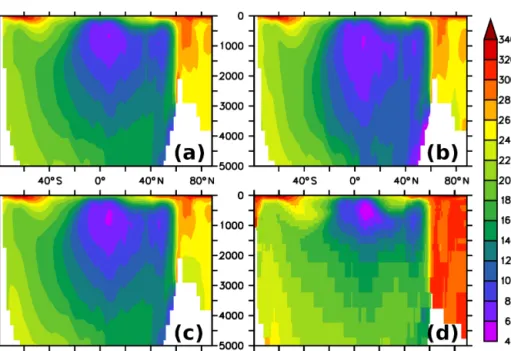
Figure A3.Meridional section of annual mean oxygen concentration (mmol O₂m⁻³) (zonally averaged). Panels(a),(b)and(c)refer to simulations FMCD, CON and E&G, respectively. Panel(d)shows observations (Garcia et al., 2010b).

(12)

Figure A4.Ice-covered months in a year. Panel(a)refers to a 1990 to 2000 average derived from the Rayner et al. (2003) global analysis.

Panel(b)refers to the simulation FMCD.

(13)

port by Andreas Oschlies. J. G. acknowledges funding by Deutsche Forschungsgemeinschaft via the project “Impact of eddy parameterizations on the simulated response of Southern Ocean air–sea CO₂fluxes to wind stress changes in IPCC-type ocean models” and BIOACID II (grant 03F0655A). Heiner Dietze and Ulrike Löptien acknowledge support by Deutsche Forschungsgemeinschaft SPP 1158, “Glacial/Interglacial Hydrographic Structures and Nutrient Utilization in the Pacific Southern Ocean – A Data and Modeling Approach”. Integrations were performed on the computer clusters weil.geomar.de, wafa.geomar.de, and other hardware from the GEOMAR Helmholtz Centre for Ocean Research, Germany, Kiel, FB2/BM. Further, we used the scalar HPC cluster of the NEC System at the Christian-Albrechts-Universität zu Kiel which is co-funded by GEOMAR. Reviews by P. R. Gent and one anonymous reviewer helped to improve the original manuscript.

The authors wish to acknowledge use of the Ferret program for analysis and graphics in this paper. Ferret is a product of NOAA’s Pacific Marine Environmental Laboratory. (Information is available at http://ferret.pmel.noaa.gov/Ferret/).

The article processing charges for this open-access publication were covered by a Research

Centre of the Helmholtz Association.

Edited by: G. Herndl

Reviewed by: P. R. Gent and one anonymous referee

References

Anderson, R. F., Ali, S., Bradtmiller, L. I., Nielsen, S. H. H., Fleisher, M. Q., Anderson, B. E., and Burckle, L. H.:

Wind-driven upwelling in the Southern Ocean and the deglacial rise in atmospheric CO₂, Science, 323, 1443–1448, doi:10.1126/science.1167441, 2009.

Bhattachan, A., D’Odorico, P., Baddock, M. C., Zobeck, T. M., Okin, G. S., and Cassar, N.: The Southern Kalahari: a potential new dust source in the Southern Hemisphere?, Environ. Res.

Lett., 7, 024001, doi:10.1088/1748-9326/7/2/024001, 2012.

Bishop, S. P., Gent, P. R., Bryan, F. O., Thompson, A. F., and Abernathey, R.: Southern Ocean Overturning Compensation in an Eddy-Resolving Climate Simulation, J. Phys. Oceanogr., 46, 1575–1592, doi:10.1175/JPO-D-15-0177.1, 2016.

Böning, C. W., Dispert, A., Visbeck, M., Rintoul, S. R., and Schwarzkopf, F. U.: The response of the Antarctic Circumpolar

the Baltic Sea, Ocean Sci., 12, 977–986, doi:10.5194/os-12-977- 2016, 2016.

Dietze, H., Getzlaff, J., and Löptien, U.: Data set to: ”Simulat- ing natural carbon sequestration in the Southern Ocean: on uncertainties associated with eddy parameterizations and iron deposition”, available at: http://thredds.geomar.de/thredds/catalog/

open_access/dietze_et_al_2017_bg/catalog.html, 2017.

Dufour, C. O., Griffies, S. M., de Souza, G. F., Frenger, I., Morri- son, A. K., Palter, J. B., Sarmiento, J. L., Galbraith, E. D., Dunne, J. P., Anerson, W. G., and Slater, R. D.: Role of mesoscale eddies in cross-frontal transport of heat and biogeochemical trac- ers in the Southern Ocean, J. Phys. Oceanogr., 45, 3057–3081, doi:10.1175/JPO-D-14-0240.1, 2015.

Duggen, S., Olgun, N., Croot, P., Hoffmann, L., Dietze, H., Delmelle, P., and Teschner, C.: The role of airborne volcanic ash for the surface ocean biogeochemical iron-cycle: a review, Bio- geosciences, 7, 827–844, doi:10.5194/bg-7-827-2010, 2010.

Eden, C. and Greatbatch, R.: Towards a mesoscale eddy closure, Ocean Model., 20, 223–239, doi:10.1016/j.ocemod.2007.09.002, 2008.

Eden, C., Jochum, M., and Danabasoglu, G.: Effects of different closures for thickness diffusivity, Ocean Model., 26, 47–59, doi:10.1016/j.ocemod.2008.08.004, 2009.

Eyring, V., Bony, S., Meehl, G. A., Senior, C. A., Stevens, B., Stouffer, R. J., and Taylor, K. E.: Overview of the Coupled Model Intercomparison Project Phase 6 (CMIP6) experimental design and organization, Geosci. Model Dev., 9, 1937–1958, doi:10.5194/gmd-9-1937-2016, 2016.

Farneti, R. and Gent, P. R.: The effects of the eddy-induced advection coefficient in a coarse-resolution coupled climate model, Ocean Model., 39, 135–145, doi:10.1016/j.ocemod.2011.02.005, 2011.

Frants, M., Holzer, M., DeVries, T., and Matear, R.: Constraints on the global marine iron cycle from a simple inverse model, J. Geo- phys. Res.-Biogeosci., 121, 28–51, doi:10.1002/2015JG003111, 2016.

Frenger, I., Gruber, N., Knutti, R., and Münnich, M.: Imprint of Southern Ocean eddies on winds, clouds and rainfall, Nature Geosci., 6, 608–612, doi:10.1038/ngeo1863, 2013.

Frölicher, T. L., Sarmiento, J. L., Paynter, D. J., Dunne, J. P., Krast- ing, J. P., and Winton, M.: Dominance of the Southern Ocean in anthropogenic carbon and heat uptake in CMIP5 models, J.

Climate, 28, 862–886, doi:10.1175/JCLI-D-14-00117.1, 2015.

(14)

Galbraith, E. D., Gnanadesikan, A., Dunne, J. P., and His- cock, M. R.: Regional impacts of iron-light colimitation in a global biogeochemical model, Biogeosciences, 7, 1043–1064, doi:10.5194/bg-7-1043-2010, 2010.

Garcia, H. E., Locarnini, R. A., Boyer, T. P., and Antonov, J. I.:

World Ocean Atlas 2009, Volume 4: Nutrients (phosphate, nitrate, silicate), edited by: Levitus, S., NOAA Atlas NESDIS 71, U.S. Government Printing Office, Washington, D.C., 398 pp., 2010.

Garcia, H. E., Locarnini, R. A., Boyer, T. P., and Antonov, J. I.:

World Ocean Antlas 2009, Volume 3: Dissolved Oxygen, Ap- paren Oxygen Utilization, and Oxygen Saturation, edited by:

Levitus, S., NOAA Atlas NESDIS 70, U.S. Government Print- ing Office, Washington, D.C., 344 pp., 2010.

Gent, P. R.: Effects of Southern Hemispheric Wind Changes on the Meridional Overturnig Circulation in Ocean Models, Annu.

Rev. Mar. Sci., 8, 79–94, doi:10.1146/annurev-marine-122414- 033929, 2016.

Gent, P. R. and Danabasoglu, G.: Response to increasing South- ern Hemisphere winds in CCSM4, J. Climate, 24, 4992–4998, doi:10.1175/JCLI-D-10-05011.1, 2011.

Gent, P. R.: The Gent-McWilliams parameterization: 20/20 hindsight, Ocean Model., 39, 2–9, doi:10.1016/j.ocemod.2010.08.002, 2011.

Gent, P. R. and McWilliams, J. C.: Isopycnal mixing in ocean circulation models, J. Phys. Oceanogr., 20, 150–155, doi:10.1175/1520-0485(1990)020<0150:IMIOCM>2.0.CO;2, 1990.

Gent, P. R., Willebrand, J., McDougall, T. J., and McWilliams, J. C.:

Parameterizing eddy-induced tracer transports in ocean circulation models, J. Phys. Oceanogr., 25, 463–474, doi:10.1175/1520- 0485(1995)025<0463:PEITTI>2.0.CO;2, 1995.

Getzlaff, J. and Dietze, H.: Effects of increased isopycnal diffusivity mimicking the unresolved equatorial intermediate current system in an earth system climate model, Geophys. Res. Lett., 40, 2166–

2170, doi:10.1002/grl.50419, 2013.

Getzlaff, J., Dietze, H., and Oschlies, A.: Simulated effects of southern hemispheric wind changes on the Pacific oxygen minimum zone, Geophys. Res. Lett., 43, 728–734, doi:10.1002/2015GL066841, 2016.

Gnanadesikan, A., Dixon, K. W., Griffies, S. M., Balaji, V., Bar- reiro, M., Beesley, J. A., Cooke, W. F., Delworth, T. L., Gerdes, R., Harrison, M. J., Held, I. M., Hurlin, W. J., Lee, H. C., Liang, Z., Nong, G., Pacanowski, R. C., Rosati, A., Russell, J., Samuels, B. L., Song, Q., Spelman, M. J., Stouffer, R. J., Sweeney, C. O., Vecchi, G., Winton, M., Wittenberg, A. T., Zeng, F., Zhang, R., and Dunne, J. P.: GFDL’s CM2 Global Coupled Climate Models.

Part II: The Baseline Ocean Simulation, J. Climate, 19, 675–697, doi:10.1175/JCLI3630.1, 2005.

Griffies, S. M., Gnanadesikan, A., Dixon, K. W., Dunne, J. P., Gerdes, R., Harrison, M. J., Rosati, A., Russell, J. L., Samuels, B. L., Spelman, M. J., Winton, M., and Zhang, R.: Formulation of an ocean model for global climate simulations, Ocean Sci., 1, 45–79, doi:10.5194/os-1-45-2005, 2005.

Hall, A. and Visbeck, M.: Synchronous variability in the Southern Hemisphere atmosphere, sea ice, and ocean resulting from the Annular Mode, J. Climate, 15, 3043–3057, doi:10.1175/1520- 0442(2002)015<3043:SVITSH>2.0.CO;2, 2002.

Hallberg, R. and Gnanadesikan, A.: The role of eddies in determin- ing the structure and response of the wind-driven Southern Hemi- sphere overturning: Initial results from the Modelling Eddies in the Southern Ocean project, J. Phys. Oceanogr., 36, 3312–3330, doi:10.1175/JPO2980.1, 2006

Hogg, A. McC., Meredith, M. P., Blundell, J. R., and Wilson, C.:

Eddy heat flux in the Southern Ocean: Response to variable wind forcing, J. Climate, 21, 608–620, doi:10.1175/2007JCLI1925.1, 2008.

Johnson, K. S., Gordon, R. M., and Coale, K. H.: What controls dissolved iron concentrations in the world ocean?, Mar. Chem., 57, 137–161, doi:10.1016/S0304-4203(97)00043-1, 1997.

Krishnamurthy, A., Moore, J. K., Mahowald, N., Luo, C., Doney, S. C., Lindsay, K., and Zender, C. S.: Impacts of increasing anthropogenic soluble iron and nitrogen deposition on ocean biogeochemistry, Glob. Biogeochem. Cy., 23, GB3016, doi:10.1029/2008GB003440, 2009.

Landschützer, P., Gruber, N., Haumann, F. A., Rödenbeck, C., Bakker, D. C. E, van Heuven, S., Hoppema, M., Metzl, N., Sweeny, C., Takahashi, T., Tilbrook, B., and R. Wanninkhof (2015). The reinvigoration of the Southern Ocean carbon sink.

Science, 349, 6253, 1221–1224. doi:10.1126/science.aab2620, 2015.

Large, W. G. and Yeager, S.: Diurnal to decadal global forcing for ocean and sea-ice models: the datasets and flux climatologies, NCAR Technical Note: NCAR/TN-460+STR, CGD Division of the National Centre for Atmospheric Research, 2004.

Lenton, A. and Matear, R. J.: Role of the southern annular mode (SAM) in Southern Ocean CO₂uptake, Global Biogeochem. Cy., 21, GB2016, doi:10.1029/2006GB002714, 2007.

Lenton, A., Tilbrook, B., Law, R. M., Bakker, D., Doney, S. C., Gruber, N., Ishii, M., Hoppema, M., Lovenduski, N. S., Matear, R. J., McNeil, B. I., Metzl, N., Mikaloff Fletcher, S. E., Monteiro, P. M. S., Rödenbeck, C., Sweeney, C., and Takahashi, T.: Sea- air CO₂fluxes in the Southern Ocean for the period 1990–2009, Biogeosciences, 10, 4037–4054, doi:10.5194/bg-10-4037-2013, 2013.

Le Quéré, C., Takahashi, T., Buitenhuis, E. T., Rödenbeck, C., and Sutherland, S. C.: Saturation of the Southern Ocean CO₂ sink due to recent climate change, Science, 316, 1735–1738, doi:10.1126/science.1136188, 2007.

Locarnini, R. A., Mishonov, A. V., Antonov, J. I., Boyer, T. P., and Garcia, H. E.: World Ocean Atlas 2009, Volume 1: Temperature, edited by: Levitus, S., NOAA Atlas NESDIS 68, U.S. Govern- ment Printing Office, Washingto, D.C., 184 pp., 2010.

Löptien, U. and Dietze, H.: Constraining parameters in marine pelagic ecosystem models – is it actually feasible with typical observations of standing stocks?, Ocean Sci., 11, 573–590, doi:10.5194/os-11-573-2015, 2015.

Lovenduski, N. S., Gruber, N., Doney, S. C., and Lima, I. D.: En- hanced CO₂outgassing in the Southern Ocean from a positive phase of the Southern Annular Mode, Global Biogeochem. Cy., 21, GB2026, doi:10.1029/2006GB002900, 2007.

Lovenduski, N. S., Gruber, N., and Doney, S. C.: Toward a mechanistic understanding of the decadal trends in the South- ern Ocean carbon sink, Global Biogeochem. Cy., 22, GB3016, doi:10.1029/2007GB003139, 2008.

Lovenduski, N. S., Long, M. C., Gent, P. R., and Lindsay, K.:

Multi-decadal trends in the advection and mixing of natural car-

(15)

Marshall, G. J.: Trends in the Southern Annular Mode from observations and reanalyses, J. Climate, 16, 4134–4143, doi:10.1175/1520-0442(2003)016<4134:TITSAM>2.0.CO;2, 2003.

Marshall, J. and Speer, K.: Closure of the meridional overturning circulation through Southern Ocean upwelling, Nature Geosci., 5, 171–180, doi:10.1038/ngeo1391, 2012.

McDougall, T. J. and Church, J. A.: Pitfalls with the Nu- merical Representation of Isopycnal and Diapycnal Mix- ing, J. Phys. Oceanogr., 16, 196–199, doi:10.1175/1520- 0485(1986)016<0196:PWTNRO>2.0.CO;2, 1985.

Metzl, N.: Decadal increase of oceanic carbon dioxide in Southern Indian Ocean surface waters (1991–2007), Deep-Sea Res. II, 56, 607–619, doi:10.1016/j.dsr2.2008.12.007, 2009.

Olgun, N., Duggen, S., Croot, P. L., Delmelle, P., Dietze, H., Schacht, U., Oskarsson, N., Siebe, C., Auer, A., and Garbe- Schönberg, D.: The role of airborne volcanic ash from sub- duction zone and hot spot volcanoes and related iron fluxes into the Pacific Ocean, Global Biogeochem. Cy., 25, 1–15, doi:10.1029/2009GB003761, 2011.

Orr, J. C., Najjar, R. G., Aumount, O., Bopp, L., Bullister, J.

L., Danabasoglu, G., Doney, S. C., Dunne, J. P., Dutay, J.- C., Graven, H., Griffies, S. M., John, J. G., Joos, F., Levin, I., Lindsay, K., Matear, R. J., McKinley, G. A., Mouchet, A., Oschlies, A., Romanou, A., Schlitzer, R., Tagliabue, A., Tan- hua, T., and Yool, A.: Biogeochemical protocols and diagnostics for the CMIP6 Ocean Model Intercomparison Project (OMIP), Geosci. Model Dev. Discuss., doi:10.5194/gmd-2016-155, in review, 2016.

Polvani, L. M., Waugh, D. W., Correa, G. J. P., and Son, S.-W.: Stratospheric Ozone Depletion: The Main Driver of Twentieth-Century Atmospheric Circulation Changes in the Southern Hemisphere, J. Climate, 24, 795–812, doi:10.1175/2010JCLI3772.1, 2011.

Rayner, N. A., Parker, D. P., Horton, E. B., Folland, C. K., Alexan- der, L. V., Rowell, D. P., Kent, E. C., and Kaplan, A.: Global analyses of sea surface temperature, sea ice, and night marine air temperature since the late nineteenth century, J. Geophys. Res., 108, 2156–2202, doi:10.1029/2002JD002670, 2003.

Redi, M. H.: Oceanic isopycnal mixing by coordinate rotation, J. Phys. Oceanogr., 12, 1154–1158, doi:10.1175/1520- 0485(1982)012<1154:OIMBCR>2.0.CO;2, 1982.

Resing, J. A., Sedwick, P. N., German, C. R., Jenkins, W. J., Moffett, J. W., Sohst, B. M., and Tagliabue, A.: Basin-scale transports of

Sigman, D. M. and Boyle, E. A.: Glacial/interglacial varia- tions in atmospheric carbon dioxide, Nature, 407, 859–869, doi:10.1038/35038000, 2000.

Simpkins, G. R. and Karpechko, A. Y.: Sensitivity of the southern annular mode to greenhouse gas emission scenarios, Clim. Dy- nam., 38, 563–572, doi:10.1007/s00382-011-1121-2, 2012.

Smetacek, V., Klaas, C., Strass, V. H., Assmy, P., Montresor, M., Cisewski, B., Savoye, N., Webb, A., d’Ovidio, F., Arrieta, J. M., Bathmann, U., Bellerby, R., Berg, G. M., Croot, P., Gonza- lez, S., Henjes, J., Herndl, G. J., Hoffmann, L. J., Leach, H., Losch, M., Mills, M. M., Neill, C., Peeken, I., Röttgers, R., Sachs, O., Sauter, E., Schmidt, M. M., Schwarz, J., Terbr|’uggen, A., and Wolf-Gladrow, D.: Deep carbon export from a South- ern Ocean iron-fertilized diatom bloom, Nature, 487, 313–319, doi:10.1038/nature11229, 2012.

Smith, S. L., Yamanaka, Y., Pahlow, M., and Oschlies, A.: Optimal uptake kinetics: physiological acclimation explains the pattern of nitrate uptake by phytoplankton in the ocean, Mar. Ecol. Prog.

Ser., 384, 1–12, doi:10.3354/meps08022, 2009.

Song, H., Marshall, J., Munro, D. R., Dutkiewicz, S., Sweeny, C., McGillicuddy, D. J., and Hausmann, U.: Mesoscale modulation of air-sea CO₂flux in Drake Passage, J. Geophys. Res.-Oceans, 121, 6635–6649, doi:10.1002/2016JC011714, 2016.

Swart, N. C., Fyfe, J. C., Saenko, O. A., and Eby, M.: Wind-driven changes in the ocean carbon sink, Biogeosciences, 11, 6107–

6117, doi:10.5194/bg-11-6107-2014, 2014.

Tagliabue, A., Aumont, O., and Bopp, L.: The impact of different external sources of iron on the global carbon cycle, Geophys.

Res. Lett., 41, 920–926, doi:10.1002/2013GL059059, 2014.

Tagliabue, A., Aumont, O., DeAth, R., Dunne, J. D., Dutkiewicz, S., Galbraith, E., Misumi, K., Moore, J. K., Ridgwell, A., Sher- man, E., Stock, C., Vichi, M., Völker, C., and Yool, A.: How well do global ocean biogeochemistry models simulate dissolved iron distributions?, Global Biogeochem. Cy., 30, 149–

174, doi:10.1002/2015GB005289, 2016.

Takahashi, T., Sutherland, S. C., Wanninkhof, R., Sweeney, C., Feely, R. A., Chipman, D. W., Hales, B., Friederich, G., Chavez, F., Sabine, C., Watson, A., Bakker, D. C. E., Schuster, U., Metzl, N., Yoshikawa-Inoue, H., Ishii, M., Midorikawa, T., Nojiri, Y., Kortzinger, A., Steinhoff, T., Hoppema, M., Olafsson, J., Arnar- son, T. S., Tilbrook, B., Johannessen, T., Olsen, A., Bellerby, R., Wong, C. S., Delille, B., Bates, N. R., and De Baar, H. J. W.: Cli- matological mean and decadal change in surface ocean pCO₂,

(16)

and net sea-air CO₂flux over the global oceans, Deep-Sea Res.

II, 56, 554–577, doi:10.1016/j.dsr2.2008.12.009, 2009.

Thompson, D. W. L. and Solomon, S.: Interpretation of recent Southern Hemisphere climate change, Science, 296, 895–899, doi:10.1126/science.1069270, 2002.

Verdy, A., Dutkiewicz, S., Follows, M. J., Marshall, J., and Czaja, A.: Carbon dioxide and oxygen fluxes in the Southern Ocean:

Mechanisms of interannual variability, Global Biogeochem. Cy., 21, GB2020, doi:10.1029/2006GB002916, 2007.

Veronis, G.: The role of models in tracer studies, in: Numerical Models of the Ocean Circulation, edited by: Reid, R. O., Na- tional Academy of Science, Washington, DC, 133–146, 1975.

Viebahn, J. and Eden, C.: Towards the impact of eddies an the response of the Southern Ocean to climate change, Ocean Model., 34, 150–165, doi:10.1016/j.ocemod.2010.05.005, 2010.

Völker, C. and Tagliabue, A.: Modeling organic iron-binding lig- ands in a three-dimensional biogeochemical ocean model, Mar.

Chem., 173, 67–77, doi:10.1016/j.marchem.2014.11.008, 2015.

Xue, L., Gao, L., Cai, W.-J., Yu, W., and Wei, M.: Response of sea surface fugacity of CO₂to the SAM shift south of Tasma- nia: Regional differences, Geophys. Res. Lett., 42, 3973–3979, doi:10.1002/2015GL063926, 2015.

Zickfeld, K., Fyfe, J. C., Saenko, O. A., Eby, M., and Weaver, A. J.:

Response of the global carbon cycle to human-induced changes in Southern Hemisphere winds, Geophys. Res. Lett., 34, L12712, doi:10.1029/2006GL028797, 2007.