Predicting muscle tissue response from calibrated component models and histology-based finite element models

(1)

Research Collection

Journal Article

Predicting muscle tissue response from calibrated component models and histology-based finite element models

Author(s):

Kuravi, Ramachandra; Leichsenring, Kay; Trostorf, Robin; Morales-Orcajo, Enrique; Böl, Markus; Ehret, Alexander E.

Publication Date:

2021-05

Permanent Link:

https://doi.org/10.3929/ethz-b-000469373

Originally published in:

Journal of the Mechanical Behavior of Biomedical Materials 117, http://doi.org/10.1016/

j.jmbbm.2021.104375

Rights / License:

Creative Commons Attribution 4.0 International

This page was generated automatically upon download from the ETH Zurich Research Collection. For more information please consult the Terms of use.

ETH Library

(2)

journal of the mechanical behavior of biomedical materials 117 (2021) 104375

Available online 3 February 2021

Contents lists available atScienceDirect

Journal of the Mechanical Behavior of Biomedical Materials

journal homepage:www.elsevier.com/locate/jmbbm

Research paper

Predicting muscle tissue response from calibrated component models and histology-based finite element models

Ramachandra Kuravi

^a^,^b

, Kay Leichsenring

^c

, Robin Trostorf

^c

, Enrique Morales-Orcajo

^c

, Markus Böl

^c^,∗

, Alexander E. Ehret

^a^,^b^,∗∗

aEmpa, Swiss Federal Laboratories for Materials Science and Technology, Überlandstrasse 129, CH-8600, Dübendorf, Switzerland

bETH Zurich, Institute for Mechanical Systems, Leonhardstrasse 21, CH-8092, Zürich, Switzerland

cTechnische Universität Braunschweig, Institute of Mechanics and Adaptronics, Langer Kamp 8, D-38106 Braunschweig, Germany

A R T I C L E I N F O

Keywords:

Skeletal muscle Extracellular matrix Microstructure

Inverse finite element method Computational modelling Constitutive equations

A B S T R A C T

Skeletal muscle is an anisotropic soft biological tissue composed of muscle fibres embedded in a structurally complex, hierarchically organised extracellular matrix. In a recent work (Kuravi et al., 2021) we have developed 3D finite element models from series of histological sections. Moreover, based on decellularisation of fresh tissue samples, a novel set of experimental data on the direction dependent mechanical properties of collagenous ECM was established (Kohn et al., 2021). Together with existing information on the material properties of single muscle fibres, the combination of these techniques allows computing predictions of the composite tissue response. To this end, an inverse finite element procedure is proposed in the present work to calibrate a constitutive model of the extracellular matrix, and supplementary biaxial tensile tests on fresh and decellularised tissues are performed for model validation. The results of this rigorously predictive and thus unforgiving strategy suggest that the prediction of the tissue response from the individual characteristics of muscle cells and decellularised tissue is only possible within clear limits. While orders of magnitude are well matched, and the qualitative behaviour in a wide range of load cases is largely captured, the existing deviations point at potentially missing components of the model and highlight the incomplete experimental information in bottom-up multiscale approaches to model skeletal muscle tissue.

1. Introduction

Mathematical and computational modelling of skeletal muscle tissues poses a special challenge due to the composition, complex spatial distribution and orientation of its constituents, and their respective internal hierarchical structure, which altogether contribute to the overall motion, force generation and gait stabilising characteristics of skeletal muscle. The tissue is predominantly comprised of long, multi-nucleated excitable muscle fibres grouped into fascicles to finally form muscles (Barrett et al.,2016;Lieber,2002). This hierarchy is established by collagenous layers referred to as endomysium, perimysium and epimy- sium that wrap fibres, fascicles and muscles, respectively (Barrett et al., 2016;Lieber,2002). These layers form a substantial part of the extracellular matrix (ECM) and constitute 1%–10% (Kjær,2004) of the muscle dry weight. The layers vary in their composition, structure and also in their respective mass fractions. For instance, endomysium exhibits a thin continuous random network-like structure shared by adjacent

∗ Corresponding author.

∗∗ Corresponding author at: Empa, Swiss Federal Laboratories for Materials Science and Technology, Überlandstrasse 129, CH-8600, Dübendorf, Switzerland.

E-mail addresses: m.boel@tu-braunschweig.de(M. Böl),alexander.ehret@empa.ch(A.E. Ehret).

muscle fibres (Purslow and Trotter, 1994) and constitutes 0.47%–

1.2% (Purslow, 2010) of muscle dry weight, while perimysium is observed in thick bands with more discrete interfaces (Passerieux et al., 2007) and discernible orientations (Purslow,2008). Differences are also hypothesised in their respective deformation mechanisms (Purslow, 2010; Takaza et al., 2014). Experimental evidence suggests a strong relation between this complex internal microstructure and the mechanical behaviour observed at tissue scale, such as a pronounced tension–compression asymmetry (Mohammadkhah et al.,2016;Gindre et al.,2013), local deformation mechanisms (Mohammadkhah et al., 2018;Takaza et al.,2014), and complex material symmetry (Böl et al., 2014).

Commonly employed continuum constitutive models inspired by muscle physiology use lumped representations of constituents by sim- plifying the muscle tissue geometry as a fibre-reinforced material ex- hibiting transverse isotropy (Röhrle and Pullan,2007;Blemker et al., 2005;Böl et al.,2011; Blemker and Delp,2005). While such models

https://doi.org/10.1016/j.jmbbm.2021.104375

Received 3 October 2020; Received in revised form 21 December 2020; Accepted 27 January 2021

(3)

offer ease of numerical implementation and provide an ‘averaged’

macroscopic response, they are unable to relate this response to internal changes of microstructure, to the distribution of stresses and strains among components, or to their interactions. In this regard, the use of multi-scale models encompassing the microstructure, with distinct continuum representations for the individual constituents, i.e. muscle fibres and ECM, have recently gained importance to explore the effect of microscopic properties on the macroscopic behaviour (Sharafi and Blemker,2010; Bleiler et al., 2019;Gindre et al., 2013), and to address medical questions in relation to muscle pathologies such as Duchenne muscular dystrophy (DMD) (Briguet et al., 2004; Emery, 2002), spasticity (Lieber et al.,2004) and deep pressure ulcers (Steke- lenburg et al.,2006). While tension–compression asymmetry was ex- plored in Gindre et al. (2013) using a structural model, more involved finite element (FE) based micromechanical models were employed to explore the microstructure dependent longitudinal shear modulus (Sharafi and Blemker,2010), the effect of DMD-related tissue alterations on the damage susceptibility (Virgilio et al.,2015), and the component specific contributions to passive muscle behaviour (Mar- cucci et al., 2019). Multi-scale considerations were also utilised in conjunction with homogenisation frameworks to develop continuum constitutive models (Spyrou et al., 2017, 2019; Bleiler et al.,2019).

However, these microstructure models are based on either information from single histological sections of muscle tissue cut perpendicular to the muscle fibres (Marcucci et al.,2017, 2019;Sharafi and Blemker, 2010, 2011), on artificially generated cross-sections (Virgilio et al., 2015;Spyrou et al.,2017,2019) or on idealised tissue geometries in combination with the assumption of affinity (Gindre et al.,2013;Bleiler et al.,2019). Hence, these current approaches do not incorporate mi- crostructural changes along the fibre axis, which break symmetry and add additional model complexity. In a recent study we have reported on the effect of including this complexity by comparing the responses of an extruded micro-scale FE model and full 3D models for various load cases (Kuravi et al.,2021).

While there are comprehensive experimental data sets on tissue scale passive behaviour of skeletal muscle, e.g. under uniaxial tension (e.g. Calvo et al., 2010; Morrow et al., 2010; Mohammadkhah et al.,2016;Takaza et al.,2013a,2014;Nie et al.,2011;Gras et al., 2012,2013), unconfined and semi-confined compression (Van Loocke et al.,2006;Böl et al.,2012;Van Loocke et al.,2009;Chawla et al., 2009; Morrow et al., 2010; Takaza et al., 2014,2013b; Van Loocke et al.,2008;Böl et al.,2014,2016), shear (Morrow et al.,2010;van Turnhout et al., 2005) as well as on single muscle fibres (Rehorn et al.,2014;Böl et al.,2019;Meyer et al.,2011;Toursel et al.,2002;

Meyer and Lieber,2011), the mechanical characteristics of ECM have remained relatively unexplored (Lewis and Purslow,1989;Lewis et al., 1991;Purslow and Trotter,1994), and even more, direct experimental information on the mechanical inter-component interactions is missing.

Towards shedding light on the anisotropic mechanical behaviour of the isolated collagenous ECM, we have recently completed a comprehensive study on decellularised muscle samples (Kohn et al.,2021). In the present contribution these novel data on ECM material characteristics are supplemented by equibiaxial tests and incorporated in detailed micro-structural FE models (Kuravi et al., 2021) to investigate the anisotropic mechanical behaviour of skeletal muscle tissues. To this end, ECM is associated with a constitutive material model inspired from its physiology, and simulations on virtual, decellularised muscle samples are performed in order to estimate the related material parameters through inverse FE analysis. The calibrated ECM FE model is combined with the muscle fibres, and the response of the composite muscle samples under various loading conditions is simulated. These predictions are compared with existing experimental data and a new set of equibiaxial extension data on fresh porcine muscle. Finally, the model is used to study effects of sample size and the characteristics of the fibre–ECM interface.

Table 1

Biaxial tension experiments conducted within this study.𝐿₁and𝐿₂are the longitudinal and transversal sample lengths, respectively, and𝑇 defines the sample thickness.

Group Sample no. Untreated NaOH-treated

𝑇 𝐿₁ 𝐿₂ 𝑇 𝐿₁ 𝐿₂

[mm] [mm] [mm] [mm] [mm] [mm]

G₁

I 5.9 38.4 36.4 – – –

II 5.5 39.3 39.9 – – –

III 5.2 38.0 42.3 – – –

IV 4.4 36.3 38.0 – – –

V 5.1 37.1 41.0 – – –

VI 5.6 39.3 39.7 – – –

G₂

VII – – – 3.0 39.0 38.6

VIII – – – 3.6 39.5 37.3

IX – – – 3.1 42.0 39.9

X – – – 3.1 38.3 39.4

XI – – – 3.7 39.2 41.4

XII – – – 3.3 39.9 37.6

XIII – – – 3.6 39.1 39.6

XIV – – – 3.3 39.5 37.8

mean 5.3 38.1 39.5 3.3 39.6 38.9

±

s.d. 0.5 1.1 1.9 0.2 1.0 1.3

2. Methods

2.1. Equibiaxial testing of muscle and ECM 2.1.1. Ethical approval

The study was exempted from ethical committee review according to national regulations (German Animal Welfare Act), as porcine skeletal muscles of healthy, female domestic pigs were obtained from a slaughterhouse immediately after animal sacrifice.

2.1.2. Sample preparation

Hind legs (𝑛= 2) of female domestic pigs (Sus scrofa domestica, age:

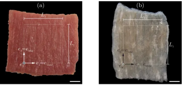
∼6 month, mass:∼90 to 100 kg) were obtained from a slaughterhouse immediately after animal sacrifice. After the legs were transported to the laboratory in a cool box at 4 ^◦C, biceps femoris muscles were excised and rectangular samples with characteristic edge lengths of approximately 60 mm and a thickness of 6 mm were cut. Care was taken to ensure that two edges of a sample were aligned parallel to the fibre orientation (Fig. 1). Further, alginate was used to stabilise the tissue during cutting with a utility cutter (Böl et al.,2014). To pre- vent rigor mortis during the preparation and storage period, the fresh muscles and samples were wrapped in cloths, soaked with Dulbecco’s phosphate-buffered saline (DPBS) at 4^◦C in a climatic chamber.

Before performing equibiaxial extension tests (𝑛 = 14) the differ- ently processed tissue samples were divided into two groups (G₁, G₂) and the specimens were trimmed to edge lengths of approximately 40 mm (Fig. 1, Table 1). The actual edge lengths (𝐿₁, 𝐿₂) in both directions were determined from digital images as mean values of two opposite sample edges and the thickness𝑇 was defined as the mean value of the thicknesses of all 4 edges. G₁comprises the fresh, untreated tissue samples as excised from the muscle, whereas G₂includes NaOH- treated samples with muscle cells removed according to a recently presented protocol (Kohn et al.,2021). In brief, the fresh samples were placed in 3% NaOH solution for 18 h. Thereafter, the treated tissues were removed from the NaOH solution and placed for 45 min in DPBS solution and then again in fresh DPBS solution for another 15 min, for more details seeKohn et al.(2021).

2.1.3. Biaxial testing equipment

Mechanical experiments were performed on a planar biaxial testing machine (Zwick GmbH & Co. KG, Germany) with four independently controllable linear actuators (Fig. 2a). Forces were measured by two load cells along each axis, with maximum load capacity of 100 N and

(4)

Fig. 1. Two types of samples used within this study: (a) Untreated fresh samples and (b) samples treated with sodium hydroxide (NaOH). The white dotted squares indicate the final sample size, trimmed to an edge length of approximately 40 mm. Scale bars: 10 mm.

Fig. 2. Experimental setup: (a) View of the tissue specimen mounted in the testing machine and (b) idealised illustrations of the marker (filled cycles) and hook (filled squares) positions. Note, the dimensions are given in millimetres, and the directions 1, 2, and 3 of the coordinate system correspond to the transversal, longitudinal, and𝑧-direction, respectively (cf. Fig. 1).

1 mN resolution, coupled to mounting devices that each consist of a U-shaped aluminium profile and a bolt holding a set of five hooks and cords (Fig. 2a). Additionally, a video extensometer (Video Exten- someter ME46, Messphysik Materials Testing GmbH, Austria) with a minimum resolution of 0.4μm was mounted above the specimens for tracking auxiliary markers on the upper side of the specimen (Fig. 2b), and whose output is used to control the movement of the actuators. A monochrome CCD camera detects the light-to-dark transitions on the surface of the samples and produces digital pixel images in 256 shades of grey. The software used for the measurement system (videoXtens, Zwick GmbH & Co. KG, Germany) processes the real time data record- ing and enables the tracking of the markers. Load cell values, actuator positions, and marker displacements were measured at 20 Hz and used for data analysis (Section2.1.5).

2.1.4. Sample processing and testing protocol

Each dissected square sample was fixed with 20 hooks (five per sample side) regularly distributed along the sample edges, with a 7.0 mm hook-to-hook distance and 5.0 mm corner hook distance (Fig. 2b), see Morales-Orcajo et al. (2018) for details. Black circular markers (diameter 1 mm) distributed in a nine-dot square grid (3 mm distance between the markers) were glued on the upper side of the specimen to

enable in-plane displacement measurements with the video extensometer (Fig. 2). The tracking area constitutes 4% of the area bound by the hooks (30×30 mm), which ensures a homogeneous stress distribution in the tracking area (Sun et al.,2005). Finally, the prepared specimen was positioned on the mounting devices of the biaxial machine, so that the muscle fibre direction was aligned with𝒆₂(Fig. 2a). To remove the weight effect and ensure the correct measurement of the initial markers distance in-plane, for all tests a preload of 10 mN was applied in both axes. The stretch-controlled experiments were realised with a strain rate of 0.5% s⁻¹ until sample failure. Due to the short test duration of a maximum of one minute, it was not necessary to moisten the sample during the experimental realisation.

2.1.5. Data analysis

Under the assumption that the deformation is homogeneous in the central region of the specimen, the two stretch ratios along and perpendicular to the visible main course of the muscle fibres were determined from the tracked displacements (e.g.Morales-Orcajo et al., 2018), and controlled to be equal in order to generate at state of equibiaxial extension, characterised through the stretch ratio𝜆. They represent the components 𝐹₁₁ and 𝐹₂₂ of the deformation gradient (cf. Section2.3) with respect to the coordinate system given inFig. 2.

(5)

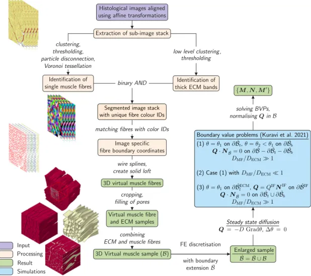
Fig. 3.Summary of all the steps involved in the development of 3D virtual muscles from histological images according toKuravi et al.(2021).

Source:Images partly adapted fromKuravi et al.(2021).

They are not principal stretches in general, due to the presence of shear in the heterogeneous, anisotropic samples.

The two perpendicularly directed forces𝑓₁and𝑓₂were determined as the averages of the two opposite force sensors, respectively, and the nominal stresses were calculated as

𝑃⁽⁹⁰⁾= 𝑓₁

𝐿₁𝑇, 𝑃⁽⁰⁾= 𝑓₂

𝐿₂𝑇 (1)

using the sample-specific dimensions (𝐿₁, 𝐿₂, 𝑇) of each specimen (Table 1). Linear interpolation between the dense data points was used in order to compute mean and standard deviation at representative values of stretch, and to represent them as nominal stress vs. stretch, i.e.𝑃−𝜆curves.

2.2. Generation of 3D FE models from histological sections

3D virtual muscle samples are either imported from existing data sets (Kuravi et al.,2021,2020) or generated from histological images as described inKuravi et al. (2021). Briefly, the following steps are performed to achieve these models: A set of pre-selected images of the histological image stack are aligned with each other through affine registration utilising auxiliary markers. A stack of square-shaped sub- images is cropped, subjected to a set of image processing operations with Fiji (Münch, 2019; Schindelin et al., 2012), and Voronoi tes- sellation is performed. This yields a segmented image stack wherein individual muscle fibres and collagenous areas are identified. Boundary coordinates of individual muscle fibres are matched across all the

segmented images and smoothly connected to form 3D virtual muscle fibres. The pore space is finally filled and attributed to the ECM, and the components are combined to a discretised muscle sample, which was meshed with tetrahedral elements (Appendix,Table A.3) such that they share same interface nodes, using FE software (Abaqus/CAE 6.14-1, Dassault Systèmes). A graphical summary of the procedure is provided inFig. 3.

The local anisotropy of the model within the muscle fibre (MF) and ECM sections is determined by solving boundary value problems (BVP) of steady state diffusion (Kuravi et al., 2021). Briefly, the boundary

𝜕of the muscle tissue sampleis subdivided into top, bottom and lateral faces (𝜕𝑡, 𝜕𝑏 and𝜕𝑙), which are in turn partitioned into fibre and ECM portions. In addition, all the internal interfaces between muscle fibres and ECM and their corresponding outward normal vector are identified as𝜕IF and𝑵_IF, respectively. Fibres and ECM are equipped with auxiliary coefficients of diffusion, and by specifying concentrations or fluxes at the boundaries and interfaces, various BVPs are analysed and the flux vectors𝑸associated with the local anisotropy are computed. To mitigate the boundary effect, BVPs were solved on extended domains (∪), obtained from 200̄ μm larger histological sections, that include boundary extensions̄of 100μm (approximately one typical fibre diameter) width at the lateral faces and a tie constraint was enforced betweenand̄(Fig. 3). The computational solution of the BVPs, implemented as heat transfer analyses in Abaqus/Standard (Abaqus 2018, Dassault Systèmes) provide for each element within the muscle fibre a unit vector that defines the local muscle fibre direction,

(6)

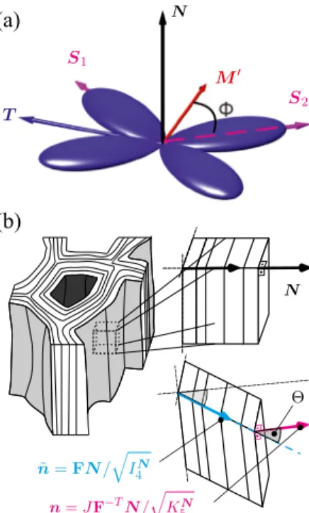
Fig. 4. Details of the ECM constitutive model. (a) Assumed collagen fibre distribution about𝑺₁and𝑺₂inclined at𝛼= 55^◦to the local muscle fibre direction𝑴^′on a surface with normal, according to the model (Holzapfel et al.,2015) with𝜅_op= 0.49,𝜅_ip= 0.15.

(b) Illustration of the characterisation of shear across ECM layers.

and within the ECM a triplet of vectors{𝑴^′,𝑵,𝑻}.𝑴^′is defined such that it is parallel to 𝑴 at the fibre–ECM interfaces𝜕IF,𝑵 specifies the local unit normal to the layered ECM structures, and𝑻 =𝑵×𝑴^′ completes these vectors to an orthonormal basis, see Kuravi et al.

(2021) for details.

2.3. Constitutive models

2.3.1. Kinematics and preliminaries

In line with the standard notation in continuum mechanics, let the configuration of a body in the reference and current (at time 𝑡) states be denoted by𝜘𝑅()and𝜘𝑡(), respectively. Each material point ofcorresponds with the positions𝑿 ∈𝜘𝑅()and𝒙∈ 𝜘𝑡(), which are linked through the mapping𝒙=𝝌_𝜘_𝑅(𝑿, 𝑡). The deformation gradient 𝐅(𝑿, 𝑡), its determinant𝐽(𝑿, 𝑡), and the right Cauchy–Green tensor𝐂(𝑿, 𝑡)are defined through

𝐅=Grad𝝌_𝜘

𝑅, 𝐽=det𝐅>0, 𝐂=𝐅^T𝐅, (2) where the dependence on place and time is understood.

For an anisotropic hyperelastic material characterised by𝑛reinforc- ing families of fibres whose direction is specified by the unit vector𝑴_𝑖, 𝑖= 1,2,…, 𝑛, the strain–energy density function (SEDF) must be a scalar isotropic tensor function of𝐂and𝐌_𝑖=𝑴_𝑖⊗𝑴_𝑖,𝑖= 1,2,…, 𝑛(Trues- dell and Noll,2004, Sec. 11). Invoking the representation theorems for isotropic scalar valued functions of symmetric tensors (Truesdell and Noll,2004), the SEDF can be given in the form, see e.g.Schröder and Neff(2003),Itskov and Aksel(2004),Ehret and Itskov(2007) 𝛹̌(𝐂,𝐌_𝑖) =𝛹(𝐼̃ ₁, 𝐼₂, 𝐼₃, 𝐼^(𝑖)

4 , 𝐾^(𝑖)

5 , 𝐼^(𝑖𝑗)

6 ), (3)

where 𝐼₁ = tr𝐂, 𝐼₂ = 𝐼₃tr𝐂⁻¹, 𝐼₃ = det𝐂 = 𝐽² are the principal invariants of𝐂, and

𝐼^(𝑖)

4 =tr(𝐂𝐌_𝑖), 𝐾^(𝑖)

5 =𝐼₃tr(𝐂⁻¹𝐌_𝑖), 𝐼^(𝑖𝑗)

6 =tr(𝐂𝐌_𝑖𝐌_𝑗), 𝑖 < 𝑗= 1,2,…, 𝑛, (4)

where typically the list of arguments of 𝛹̃ is restricted to a subset of these invariants. For materials with fibres dispersed symmetrically around the𝑛directions, generalised structure tensors𝐇_𝑝 can be defined (Advani and Tucker III,1987;Freed et al., 2005;Gasser et al., 2006). For the special case where the mean directions, say𝑺_𝑝, 𝑝 = 1,2,…, 𝑚, lie in one plane with unit normal𝑵(Fig. 4) and the dispersion can be characterised through two von-Mises type distributions that specify the in and out-of-plane distribution, the generalised structure tensors can be represented as (Holzapfel et al.,2015)

𝐇_𝑝=𝛼𝐈+𝛽𝑺_𝑝⊗𝑺_𝑝+ (1 − 3𝛼−𝛽)𝑵⊗𝑵,

𝛼= 2𝜅_op𝜅_ip, 𝛽= 2𝜅_op(1 − 2𝜅_ip), (5) where𝜅_ip ∈ [0,1∕2] and 𝜅_op ∈ [0,1∕2] represent in-plane and out- of-plane dispersion parameters, respectively. The SEDF can then be represented as

𝛹=𝛹(𝐂,̌ 𝑺_𝑝⊗𝑺_𝑝,𝑵⊗𝑵) (6)

and corresponding invariants can be defined such as 𝐼^(𝑝)

S = tr(𝐂𝐇_𝑝) (7)

that replace the invariants𝐼^(𝑝)

4 in the list of arguments of𝛹̃ in Eq.(3).

The Cauchy stress is finally obtained as 𝝈= 2𝐽⁻¹𝐅𝜕 ̌𝛹

𝜕𝐂𝐅^T. (8)

Based on these frameworks, we defined constitutive laws for muscle fibres and ECM in our previous work (Kuravi et al.,2021). The former was obtained by modification of the model inHolzapfel et al.(2000) with regard to compressibility asKuravi et al.(2021)

𝛹_MF=𝛹̌_MF(𝐂,𝑴)

=𝑐₁(𝐼₁− 3) + 𝑐₁

2𝑐₀(𝐽^−2𝑐⁰− 1) + 𝑘₁

2𝑘₂{exp(𝑘₂⟨𝐼_M− 1⟩²) − 1}, (9) where𝐼_M=tr(𝐂𝐌),⟨𝑥⟩= (|𝑥|+𝑥)∕2,𝑐₁and𝑘₁are material parameters with unit of stress, and𝑐₀and𝑘₂are positive, dimensionless constants.

The ECM model is discussed and amended in what follows.

2.3.2. Modification of the model for ECM

Drawing motivation from the experimentally observed muscle ECM microstructure, its composition and distribution in the muscle tissue (Oshima et al.,2007;Gillies and Lieber,2011;Kjær,2004;Purslow, 2008,1989;Light et al.,1985), and its resemblance with the network structures found in other tissues such as skin, cornea and arterial walls (e.g.,Limbert,2017;Pandolfi and Vasta,2012;Holzapfel et al., 2015), the ECM was modelled based on the generalised structure tensor approach inKuravi et al.(2021). In particular two local mean fibre directions

𝑺₁=𝑴^′cos𝛷+𝑻sin𝛷, 𝑺₂=𝑴^′cos𝛷−𝑻sin𝛷 (10) were considered, symmetrically inclined at an angle𝛷 to the mean muscle fibre direction𝑴^′, and lying within the plane with unit normal 𝑵, that defines the orientation of the collagenous layers (Fig. 4a). This concept was combined with the hyperelastic variant of the soft tissue model introduced inRubin and Bodner(2002), and the corresponding SEDF was given byKuravi et al.(2021)

𝛹̌_ECM(𝐂,𝐇₁,𝐇₂) =𝜇₀

2𝑞(𝑒^𝑞𝑔− 1), (11)

where in view of Eqs.(5)and(7) 𝑔=𝛽₁(𝐼₁− 3) + 𝛽₁

2𝛽₀(𝐽^−2𝛽⁰− 1) + ℎ₁

2ℎ₂ {⟨√

𝐼⁽¹⁾

S − 1

⟩2ℎ₂

+

⟨√

𝐼⁽²⁾

S − 1

⟩2ℎ₂}

. (12)

(7)

The now available experimental data on ECM (Kohn et al., 2021) pointed at a significant influence of shear across the layered ECM structures, which is in line with the hypothesis that the transmission of lateral forces across muscle fibres in muscle tissues is largely facilitated though shearing the ECM (Sharafi and Blemker,2011;Huijing,1999;

Purslow,2008). Therefore, the previous SEDF (Kuravi et al.,2021) is supplemented by a term that depends on a simple kinematic invariant related to the shear across ECM layers.

To this end, we consider an infinitesimal surface elementd𝐴parallel to the collagenous layers, i.e. characterised by the unit normal𝑵 = 𝑺₂×𝑺₁in the reference configuration𝜘𝑅(), that is mapped onto the aread𝑎with unit normal𝒏in deformed configuration𝜘𝑡()according to Nanson’s formula

𝒏d𝑎=𝐽 𝐅^−T𝑵d𝐴, (13)

and it follows d𝑎∕d𝐴 = 𝐽√

𝑵⋅𝐂⁻¹𝑵 = √

𝐾₅^𝑵 (Schröder and Neff, 2003). At the same time a line element of unit length along𝑵 trans- forms as 𝜆_𝑵𝒏̃ = 𝐅𝑵 with a stretch𝜆_N = √

𝑵⋅𝐂𝑵 = √ 𝐼^𝑵

4 . The deviation between the two vectors 𝒏 and𝒏̃ characterises the shear across the layers and is characterised by the angle (Fig. 4b)

𝛩= arccos (𝒏⋅𝒏) = arccos̃ (√ 𝐼₃

𝐼^𝑵

4 𝐾^𝑵

5

)

. (14)

The corresponding ‘amount of shear’𝛾is obtained as 𝛾= tan𝛩=

√ 𝐼^𝑵

4 𝐾^𝑵

5

𝐼₃ − 1 =√

𝐼_𝛾− 1, (15)

which defines the invariant𝐼_𝛾=𝐼^𝑵

4 𝐾^𝑵

5 ∕𝐼₃.

In addition to this structural term, an additional volumetric contribution (Miehe,1994) was added, penalising both volume loss and gain.

With these modifications, Eq.(12)is revised as follows

𝑔=𝑔₀(𝐂) +𝑔_S(𝐂,𝐇₁,𝐇₂) +𝑔_𝛾(𝐂,𝑵⊗𝑵), (16) where

𝑔₀(𝐂) =𝛽₁(𝐼₁− 3) + 𝛽₁

2𝛽₀(𝐽^−2𝛽⁰− 1) +𝛽₂(𝐽− ln𝐽− 1), 𝑔_S(𝐂,𝐇₁,𝐇₂) = ℎ₁

2ℎ₂ {⟨√

𝐼⁽¹⁾

S − 1

⟩2ℎ₂

+

⟨√

𝐼⁽²⁾

S − 1

⟩2ℎ₂} ,

𝑔_𝛾(𝐂,𝑵⊗𝑵) = 𝑙₁ 2𝑙₂𝛾_.^2𝑙²

(17)

Here,𝜇₀,𝑞,𝛽₀,𝛽₁,𝛽₂,ℎ₁,ℎ₂ ≥1,𝑙₁, and𝑙₂≥1are positive material constants.

2.4. Numerical simulations

2.4.1. FE implementation and effective stress

For mechanical analyses, the material models of muscle fibres and the ECM (Section2.3) were implemented through user-defined material subroutines (Abaqus/Standard 6.14-1,2014), wherein the local material symmetry defined by the vectors{𝑴,𝑴^′,𝑵}is introduced as state variables in the undeformed configuration.

The effective mechanical response of the muscle sample in a given BVP (Section2.4.2) was estimated using averaging theorems in finite kinematics (e.g.Hill,1972). To this end, affine displacement boundary conditions were invoked in discrete form as

𝒖^𝑎(𝑿) = (𝐅₀−𝐈)𝑿^𝑎+𝒄on𝜕, (18)

where 𝒖^𝑎 and 𝑿^𝑎 denote the displacement and the reference position of node 𝑎 on the boundary 𝜕, respectively. 𝐅₀ represents the

‘macroscopic’ deformation gradient, 𝐈is the identity tensor of second order, and𝒄 is a constant vector representing rigid translation, con- veniently set to𝟎. The volume averaged Cauchy stress tensor⟨𝝈⟩and the corresponding effective nominal stress⟨𝐏⟩(volume averaged first

Piola–Kirchhoff stress) are given as (Costanzo et al.,2005;Geers et al., 2010)

⟨𝝈⟩= 1 𝑣

∑

𝑎

𝒇^𝑎⊗𝒙^𝑎, ⟨𝐏⟩= det𝐅₀⟨𝝈⟩𝐅^−T₀ , (19) where𝑣is the current volume of the modelled domain while𝒇^𝑎and𝒙^𝑎 respectively are the total force and position of node𝑎on the boundary in the current state. The stress (19) results from volume averaging over the tissue (and not only ECM) domain. For the decellularised samples, this apparent stress is thus lower than the effective stress in the ECM, and clearly the factor in between is the volume fraction of ECM. Nevertheless, given the experimental difficulty to determine the volume and cross-section area of the decellularised muscle samples, this apparent stress is used for adjustment to the experimental data (Kohn et al.,2021).

2.4.2. Load cases

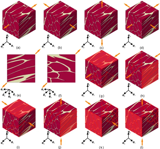
The load cases considered in this study comprise uniaxial extension with lateral contraction (UAE), uniaxial compression with lateral ex- pansion (UAC), biaxial extension with lateral contraction (BAE), and semi-confined compression (SCC), as illustrated inFigs. 5a–l.

UAE/UAC of muscle samples and ECM are simulated along the longitudinal (0^◦, Fig. 5a), transverse (90^◦, Figs. 5b,c), and oblique (45^◦, Figs. 5e,f) directions with respect to the gross muscle fibre direction, aligned with𝒆₃. BAE is considered by stretching equally along this and one orthogonal direction (Fig. 9d). Finally, three modes of semi-confined (plane strain) compression are considered (Böl et al., 2014), where compression is imposed either along the muscle fibres (mode I) or along one of the cross-fibre directions (modes II, III) while one of the transverse dimensions was held constant (Figs. 5g–

l). Noteworthy, due to the lack of symmetry we considered two cases for each mode, fixing one of the two lateral faces, respectively. The tensile/compressive stretches were specified along the loading direction(s) while stretches along the unconstrained perpendicular directions were numerically computed to achieve traction free lateral faces.

The deformation gradient is thus given as

𝐅₀=𝜆₁𝒆̂₁⊗ ̂𝒆₁+𝜆₂𝒆̂₂⊗ ̂𝒆₂+𝜆₃𝒆̂₃⊗ ̂𝒆₃ on𝜕, (20) where{̂𝒆₁, ̂𝒆₂, ̂𝒆₃}is an orthonormal basis and{𝜆₁, 𝜆₂, 𝜆₃}are the corresponding principal stretches. The basis {̂𝒆₁,𝒆̂₂,𝒆̂₃} is aligned with the global basis{𝒆₁,𝒆₂,𝒆₃}except for oblique UAE, where it is rotated by 45^◦about𝒆₁ or𝒆₂, cf.Kuravi et al.(2021). For UAE/UAC one of the stretches is prescribed, while BAE of muscle and ECM samples (Fig. 8d) is specified by prescribing𝜆₁=𝜆₃. To simulate SCC of muscle samples (Figs. 5g–l) one of the stretches is kept at unity, one is prescribed through the experimental compressive stretch, and the non-constant transverse stretch is computed.

Noteworthy, as a result of the histological preparation, there is a slight but practically unavoidable deviation between the gross muscle fibre direction and the stack axis 𝒆₃ when generating the models, cf. (Kuravi et al.,2021). Based on the computed local fibre directions𝑴 for each finite element, the mean orientation of all muscle fibres (𝑴̄_MF) with respect to the stack axis of histological images was evaluated. For the model considered here this angle was 17.06^◦. To simulate loading along and across the mean muscle fibre direction, this misalignment was allayed to<0.01^◦by rigidly rotating the cubic muscle sample with an orthogonal transformation𝐐_𝑅that maps𝑴̄_MFonto𝒆₃, a vector of the orthonormal basis{𝒆₁,𝒆₂,𝒆₃}. Please note that this rotation is not shown inFig. 5for the sake of clarity.

2.4.3. Material parameters and inverse FEM

The parameters (Table 2) of the muscle fibre model (9) were adopted fromKuravi et al.(2021), where they had been obtained by fitting the model to experiments on individual muscle fibres (Böl et al., 2019).

(8)

Fig. 5. Illustration of the considered load cases for the muscle model. (a) UAE along longitudinal (0^◦) direction. (b, c) UAE along two transverse (90^◦) directions. (d) BAE along 0^◦and 90^◦directions. (e, f) UAE along the two oblique (45^◦) directions. (g–l) Two cases of mode I (g, h), II (i, j) and III (k, l) type SCC; constrained surfaces are highlighted.

Inverse finite element (iFEM) calculations were performed to identify the set of material parameters𝒑of the ECM (Eqs.(16)and(17)).

Briefly, a set of optimal material parameters that minimises the difference between experimental and simulated responses is deduced in an iterative fashion through an optimisation algorithm driven FE analysis, see e.g.Böl et al.(2013),Takaza et al.(2013b),Böl et al.(2012) and Ahn and Kim(2010).

Experimental data for the following three load cases was adopted from Kohn et al. (2021): UAE of the decellularised muscle tissue (ECM) along the longitudinal (0^◦), oblique (45^◦), and transverse (90^◦) directions with respect to the mean muscle fibre direction (Fig. 6).

In the underlying experiments (Kohn et al.,2021), the muscle fibres were dissolved, thus leaving voids and causing the ECM structure to partially collapse. To avoid the computational effort with the consider- ation of self-contact between internal surfaces of the ECM, numerical simulations were performed on the whole muscle domainbut the fibre region (^MF) was modelled as a weak, compressible neo-Hookean material by setting𝑐₁= 0.00155 kPa,𝑐₀= 1.0and𝑘₁= 0in Eq.(9).

The optimisation algorithm to identify the parameter set (𝒑_opt) was implemented through MATLAB-based (Version 9.3, R2017b, The MathWorks Inc., Natick, MA, USA) control utilising the Nelder–Mead simplex search algorithm (Lagarias et al.,1998) embedded in MATLAB

asfminsearchfunction, minimising the objective function

(𝒑) =1 𝑛

∑𝑛 𝑖=1

√√

√

(𝑃_𝑖^exp−𝑃_𝑖^sim(𝒑))2

(𝑃_𝑖^exp)2 . (21) Here,𝑃^exp

𝑖 and𝑃^sim

𝑖 (𝒑), respectively, represent experimental and (effective) simulated nominal stresses for a given parameter set𝒑at the𝑖th increment of𝑛= 10deformation increments. Noteworthy, in line with the experiments inKohn et al.(2021) the nominal stresses represent the apparent stress that is obtained when relating the force acting on the decellularised samples to the original cross-section of the fresh tissue sample before the muscle fibres are removed. This avoids the complex determination of the void area. Fig. 7 summarises the optimisation algorithm.

In this way, the parameter set𝒑 = {

𝜇₀, 𝑞, 𝛽₀, 𝛽₁, ℎ₁, ℎ₂, 𝑙₁, 𝑙₂} was optimised whereas, to reduce the number of unknowns, the structural dispersion parameters𝜅_ip = 0.15and𝜅_op = 0.49(Eq. (5)) were pre- selected as a constitutive choice. Likewise, the parameter𝛽₂controlling compressibility was set constant (𝛽₂= 10⁵) since experimental information on volume changes was lacking. Noteworthy, this parameter affects the material compressibility, not the compressibility of the porous structure generated by removing the muscle fibres from the ECM. The

(9)

Fig. 6. An illustration of the loading directions for UAE of the ECM. (a), (b), and (c) show the longitudinal (0^◦), the 45^◦, and the transverse (90^◦) loading directions, respectively.

Fig. 7. Flowchart of the MATLAB driven FE optimisation algorithm.

optimisation was terminated when the decrease in value of the objective function was marginal over several consecutive iterations, and the simulated curves showed sound agreement with the experimental ones upon visual inspection.

2.4.4. Sample types and component interactions

At first all simulations on muscle tissue and ECM were performed with a cubic sample of 300 μm edge length generated from 5 serial histological sections and developed inKuravi et al.(2021). This model is available atKuravi et al.(2020).

InKohn et al. (2021) the effect of laterally compressing decellularised muscle samples before their response in UAE was studied. This procedure was repeated in the present study to perform BAE tests. The lateral compaction leads to flat and thin, membrane-like samples. To mimic this effect in the computational models, flat ECM models were generated by a purely geometrical operation: One of the transverse dimensions of a 300 μm cubic sample was scaled down by 𝜁 = 0.1, resulting in 90% ‘compacted’ samples (Fig. 5a), and the directions of local anisotropy were calculated from the modified vector triad {𝑴^𝑐,𝑴^′𝑐,𝑵^𝑐}as

𝑹^c= 𝑹−𝜁(𝑹⋅𝒆₂)𝒆₂

‖𝑹−𝜁(𝑹⋅𝒆₂)𝒆₂‖, 𝑹∈ {𝑴,𝑴^′,𝑵}, (22) where𝑹^𝑐∈ {𝑴^𝑐,𝑴^′𝑐,𝑵^𝑐}denotes the corresponding modified vector of 𝑹. These samples were then subjected to UAE and BAE boundary conditions as described above and illustrated inFig. 8. Note that the stress was still considered in terms of the apparent nominal stress, i.e.

force per unit undeformed cross-sectional area of the muscle sample before decellularisation.

To assess the effect of (i) muscle sample size and (ii) muscle fibre–

ECM interface properties, UAE/UAC and SCC load cases were simulated on thin samples based on a single histological section with a cross- section of 900μm ×900μm and a (physically irrelevant) thickness of 20μm (Fig. 9). These samples were obtained by ‘extrusion’ of the segmented image along the𝒆₃ direction. To investigate the influence of interfacial properties (ii), a soft intermittent layer, about 1% of muscle fibre volume fraction (≈87%) was introduced between ECM and muscle fibres, and furnished with neo-Hookean type material model by setting 𝑐̃₁ = 0.00155 kPa and 𝑐̃₀ = 1.0 in Eq. (9). The layer is

rigidly connected to both the ECM and muscle fibres at their respective interfacing surfaces through shared nodes in the discretised muscle sample.

3. Results

In what follows, the outcome of the iFEM procedure to determine the ECM material parameters is shown. Thereafter, we present the results of the numerical simulations for 90% pre-compressed ECM samples, for 300μm cubic muscle samples and for 900μm extruded muscle samples with and without an intermediate layer between muscle fibres and ECM. Finally, if available, these results are compared to experimental data. Note again that two cases of transverse and oblique loading are considered, respectively, due to the missing symmetry in the microstructure of the sample, providing two response curves (cf. Fig. 5).

3.1. Determination of ECM parameters by means of iFEM

The optimisation process was terminated when the objective function had reduced to a value of 0.02.Table 2lists the obtained parameter set𝒑_opt, which leads to accurate agreement with the corresponding experimental data for UAE in 0^◦, 45^◦, and 90^◦directions (Fig. 10).

3.2. Predictions for compressed ECM

The simulated responses of the laterally compacted ECM samples, generated by shrinking one of the lateral dimensions by 90%, is shown inFig. 11in comparison with the experimental data fromKohn et al.

(2021) and in Fig. 12 together with the new data on the biaxial response of the compacted ECM. Noteworthy, here the experimental threshold forces of 3 mN for UAE (Kohn et al., 2021) and 10 mN for BAE, with the corresponding respective averaged pre-stress of 0.076 kPa and 0.1 kPa at𝜆= 1, were included (observed as a small offset at the stress axis). This is because the simulated compaction operation caused a significantly softer initial response, and thus an extension of the toe region. Even a small threshold force can therefore become relevant and substantially change the appearance of the curve.

This soft initial region is also expected to occur in the experiments but

(10)

Fig. 8. Illustration of load cases considered for 90% pre-compressed ECM sample (Kohn et al.,2021). (a)–(c) UAE along 0^◦, 45^◦, and 90^◦directions. (d) BAE along the 0^◦and 90^◦directions.

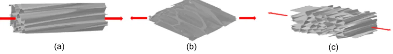
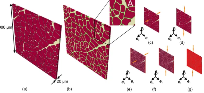
Fig. 9. Illustration of extruded muscle samples (900μm ×900μm ×20μm) subjected to SCC and the resulting response. (a) Extruded sample with muscle fibres and the ECM.

(b) Extruded sample with an intermittent layer (in green) connecting muscle fibres and the ECM. A planar magnified view is displayed in ‘A’. (c), (d) UAE of 900μm sample along fibre (0^◦) and transverse (90^◦) directions, respectively. (e)–(g) Mode I, II and III type SCC of 900μm sample, respectively. Constrained faces are highlighted.

Table 2

Material parameters of muscle fibres (Eq.(9)) and ECM (Eqs.(5),(16)).

Material Parameter Value

Muscle fibres

𝑐₀ 6.0

𝑐₁[kPa] 0.1525

𝑘₁[kPa] 2.25

𝑘₂ 0.44

ECM

𝛽₀ 1.0

𝛽₁ 0.04056

𝛽₂ 10⁵

ℎ₁ 50.25

ℎ₂ 1.03

𝑙₁ 41.54

𝑙₂ 1.379

𝜅_ip 0.15

𝜅_op 0.49

𝜇₀[kPa] 4.856

𝑞 2.184

to be ‘hidden’ because of the force threshold (see Section 4). When including this threshold, the UAE predictions closely match the experimental response. The BAE predictions, however, though predicting the order of the curves right, underpredict the experimental response.

3.3. Mechanical response of cubic muscle tissue samples

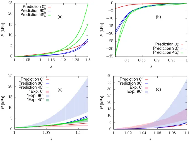
The numerically estimated effective nominal stress response of 300μm cubic muscle samples subject to UAE (𝜆= 1.3) and UAC (𝜆=

0.76) along 0^◦, 45^◦and 90^◦directions to the gross muscle fibre direction (𝒆₃) are shown inFigs. 13a and b, respectively. FromFig. 13a, it is observed that loading along 0^◦direction provides a weaker response than along the 45^◦directions up to a stretch of about 1.17, after which the latter evolves as the stiffer direction (2–3 times stiffer at𝜆= 1.3).

The weakest response is predicted along the 90^◦direction. To facilitate a fair comparison between experiments and simulations, cf.Kohn et al.

(2021), the stretches of the computed responses (Fig. 13a) were re- scaled such that the experimental initial pre-loads of 30 mN in UAE (equivalent nominal stress of 0.76 kPa) and 10 mN for BAE (equivalent nominal stress of 0.05 kPa) were matched at𝜆 = 1. (Fig. 13c). The comparison reveals that the ascending/descending order of stiffness, i.e. 90^◦>45^◦>0^◦is in line with experimental evidence (Kohn et al., 2021;Takaza et al.,2013a), while there is a mismatch in magnitude in that the predicted 0^◦direction is stiffer, whereas the computed 90^◦ direction is weaker.

Underprediction of the magnitude but a match in the order among the anisotropic stresses is also observed for the BAE response (Fig. 13d) of muscle samples along 0^◦and 90^◦directions. For instance, at𝜆= 1.1 the predicted responses reach only about 30% of the mean experimental observations.

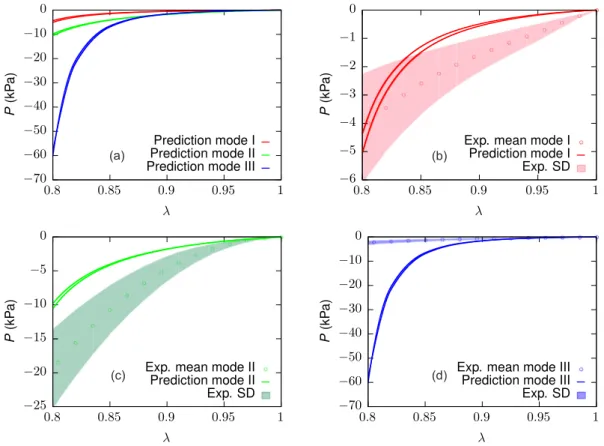
The numerically estimated effective nominal stress responses to modes I, II and III of semi-confined compression (Figs. 5g–l) are illustrated inFig. 14for a compressive stretch up to𝜆= 0.8, respectively.

Figs. 14b–d compare the predicted responses with the corresponding experimental data (Böl et al.,2014). While the responses to modes I and II compression come close to the experimental spread, the mode III

(11)

Fig. 10. Comparison of the experimental nominal stress response of the ECM (Kuravi et al.,2021) with the corresponding fitted response along (a) longitudinal (0^◦, (b) 45^◦, and (c) transverse (90^◦) directions for the optimised material parameter set𝒑_opt(1040 iterations of the algorithmFig. 7). Shaded regions represent standard deviation.

simulations (Fig. 14d) overpredict the mean experimental stress by up to an order of magnitude. This is also reflected in the order of stiffness observed among the loading directions shown inFig. 14a, where mode III > II > I, in clear contrast to mode II> I > III reported in the experiments (Böl et al.,2014).

3.4. Mechanical response of larger muscle sample

Figs. 15a,b, respectively, compare the UAE and UAC effective nominal stress responses of the extruded 900μm×900μm×20μm muscle sample with that of the full 3D 300μm cubic sample for 0^◦and 90^◦ loading directions. The responses of both the samples are similar both qualitatively and quantitatively. More precisely, in UAE (Fig. 15a) the extruded sample exhibits 20% weaker response in 0^◦direction, while it is 15%–30% stronger in the 90^◦ direction when compared to the 300μm sample at peak stretch (𝜆= 1.3). Similar deductions are made in UAC (Fig. 15b) wherein, the extruded sample is 44% weaker in 0^◦ direction and 11%–18% stronger in 90^◦direction compared to the 300 μm sample response at peak stretch (𝜆= 0.82).

Fig. 11.Comparison of the experimental nominal stress response of the 90% pre- compressed ECM (Kohn et al.,2021) with the corresponding predicted response. (a–c) UAE along longitudinal (0^◦), 45^◦, and transverse (90^◦) directions. The dashed lines (subscript𝑏) show the predicted responses when pre-loads are neglected. Shaded regions represent standard deviation.

Fig. 12. Comparison of predicted BAE response along longitudinal (0^◦) and transverse (90^◦) directions with experiments on 90% pre-compressed ECM (initial pre-load≈ 0.1 kPa). Shaded regions represent the standard deviation about their respective experimental mean response.

(12)

Fig. 13. Numerically simulated UAE, UAC and BAE response of 300μm muscle sample. (a) UAE response along 0^◦, 45^◦and 90^◦directions. (b) UAC response along 0^◦, 45^◦and 90^◦directions. (c) Comparison of UAE response with experiments (represented with pre-load≈0.76 kPa). (d) Comparison of BAE response with experiments (represented with pre-load≈0.05 kPa). Note that two cases of 45^◦and 90^◦loading were considered, respectively (cf.Fig. 5). Subscript𝑏refers to results without considering pre-loads.

Fig. 15c compares the effective nominal stress response of the 900 μm extruded sample to the 300μm sample for all three modes of SCC (Figs. 9e–f), wherein it is observed that the response is similar for modes I and II with marginal differences around≈ 10%, while in mode III the large model reaches nearly twice as high stress at𝜆= 0.82.

3.5. Effect of interactions between muscle fibres and ECM

Fig. 16 compares the behaviour of the extruded sample with and without intermittent layer under UAE, UAC and SCC load cases wherein it is observed that the latter, though weaker, closely approximates the former in both order of magnitude and ascending/descending order of stiffness. In UAE/UAC (Figs. 16a, b), they differ, respectively, by about 4%–8% and 2%–4% along 0^◦and 90^◦directions at peak stretch. In SCC (Fig. 16c), a difference of 2%, 7.5% and 4% is observed at peak stretch in modes I, II and III, respectively.

4. Discussion

In this paper, we have combined our recently published approach to generate full 3D FE models of skeletal muscle tissue from histological images and novel experimental data on the mechanical behaviour of the collagenous muscle ECM. This combination put us in a position to calibrate the models of individual components and to perform rigorous computational predictions of the composite tissue response.

Although there exist several elaborate studies that employ advanced multi-component microstructure-based models formulated either on a constitutive modelling (Spyrou et al.,2017,2019;Bleiler et al.,2019) or FE simulation basis (Sharafi and Blemker,2010;Virgilio et al.,2015;

Sharafi and Blemker,2011;Marcucci et al.,2017,2019;Spyrou et al.,

2017,2019), the first time use of the novel ECM data makes the present approach unique in that it does not contain a single parameter that should be fitted from tissue scale experiments. Accordingly, the simulations are unforgiving, and directly reveal misconceptions and erroneous assumptions when composing the tissue from its main constituents.

4.1. ECM model and parameter estimation

The comprehensive new data set (Kohn et al., 2021) suggested a remarkably stiff response when loading the decellularised samples in an angle of 45^◦ with regard to the prior axis of the fibres. We hypothesised that this behaviour could be caused by significant shear across the ECM layers, enforced through this type of loading. Hence, the constitutive model (Kuravi et al., 2021) that governs the mechanical response of the ECM in each integration point of the FE model, was amended by a shear-dependent term 𝑔_𝛾(𝐼_𝛾)(Eq. (16)) to incorporate energy associated with shear deformation through an invariant 𝐼_𝛾 (Section2.3.2). In fact, the previous version of the SEDF (Kuravi et al., 2021) assumed orthotropic material symmetry with two preferential directions, predominantly inspired by the structure of perimysium (Rowe, 1974; Purslow, 1989), and thus ignoring that endomysium exhibits a relatively random distribution (Trotter and Purslow,1992;Purslow and Trotter,1994;Purslow,2008). This was justified with the relative abundance and comparable tensile stiffness of perimysium (Light et al., 1985;Purslow,2010). However, endomysium, that coordinates force transmission across individual muscle fibres (Sharafi and Blemker, 2011;Huijing,1999;Purslow,2008), is expected to offer high shear resistance to facilitate growth and repair of sarcomeres (Purslow,2010) and load transfer in intrafascicularly terminating fibres (Sharafi and Blemker, 2010; Purslow, 2002). On the other hand, perimysium is

(13)

Fig. 14. Numerically simulated SCC response of 300μm muscle sample in comparison with experiments. (a)–(c) Comparison of mode I, mode II, and mode III type SCC response with the corresponding experimental data. (d) SCC response of the sample in modes I, II and III. Shaded regions represent standard deviation about their respective experimental mean response. Note that for each mode two cases, respectively, were considered (cf.Fig. 5).

Fig. 15. UAE and SCC responses of extruded muscle sample (900μm ×900μm ×20μm). (a), (b) respectively compare the UAE and UAC responses of the sample along 0^◦ and 90^◦directions with cubic sample (300μm) responses. (c) compares the sample responses to modes I, II and III of SCC with that of cubic muscle sample. Note that two cases of 45^◦and 90^◦loading, and of all SCC modes were considered, respectively.

Fig. 16. A comparison of UAE/UAC and SCC responses of extruded samples (900μm ×900μm ×20μm) with and without intermittent layer, wherein former is denoted with subscript ‘s’. (a), (b) respectively compare the UAE and UAC responses of both the samples while (c) compares the SCC responses. Note that two cases of 90^◦loading and SCC were considered, respectively (cf.Fig. 5).